HAL Id: inria-00604108
https://hal.inria.fr/inria-00604108
Submitted on 30 Dec 2020
HAL is a multi-disciplinary open access
archive for the deposit and dissemination of
sci-entific research documents, whether they are
pub-lished or not. The documents may come from
teaching and research institutions in France or
abroad, or from public or private research centers.
L’archive ouverte pluridisciplinaire HAL, est
destinée au dépôt et à la diffusion de documents
scientifiques de niveau recherche, publiés ou non,
émanant des établissements d’enseignement et de
recherche français ou étrangers, des laboratoires
publics ou privés.
Data Assimilation of Satellite Images within an
Oceanographic Circulation Model
Etienne Huot, Till Isambert, Isabelle Herlin, Jean-Paul Berroir, Gennady K.
Korotaev
To cite this version:
Etienne Huot, Till Isambert, Isabelle Herlin, Jean-Paul Berroir, Gennady K. Korotaev. Data
As-similation of Satellite Images within an Oceanographic Circulation Model. ICASSP 2006 - IEEE
International Conference on Acoustics, Speech and Signal Processing, May 2006, Toulouse, France.
pp.265-268, �10.1109/ICASSP.2006.1660330�. �inria-00604108�
DATA ASSIMILATION OF SATELLITE IMAGES WITHIN AN OCEANOGRAPHIC
CIRCULATION MODEL
E. Huot
†T. Isambert
‡I. Herlin
‡J.-P. Berroir
‡G. Korotaev
?†
Université de Versailles - Saint-Quentin – CETP
‡
Institut National de Recherche en Informatique et Automatique – équipe Clime
?National Academy of Sciences of Ukraine – MHI.
ABSTRACT
We tackle the problem of coupling a geophysical simulation model with data coming from image processing. It needs to define the im-age observation space and to design an operator to transform results from the image space to the model space. In this study, we use a shallow-water oceanographic circulation model developed at MHI. We propose a processing chain first based on an image processing step relying on a dedicated motion estimation operator, and then a data assimilation step of the estimated velocity. We illustrate the method on different results without and with assimilation.
1. OBJECTIVES
In the framework of numerical forecasting for the evolution of geo-physical fluid, we are interested in the assimilation of data coming from images. In order to forecast the behavior of geophysical fluids we need: a forecast model to describe the evolution of a state vari-able (generally it is a non-linear PDE system) and observations spa-tially and temporally distributed. Data assimilation provides a math-ematical solution to combine data and models. During last decades model quality increased significantly. But forecast quality is not di-rectly linked to model quality. To increase forecast quality it is also necessary to increase the amount and the quality of observations. Therefore, images – particularly images coming from spatial remote sensing – provide a huge amount of information. Using images in a data assimilation framework raises several difficulties:
1. First it is necessary to define which image space is relevant according to model specialists.
2. Then, it is necessary to construct an image operator dedi-cated to the problematic and coherent to the physical behav-ior. Moreover it is necessary to define a set of norm in order to quantify the influence of image information along the as-similation process.
3. And finally, it is necessary to construct an operator to com-pare image space and model space.
In the study presented in this paper, we are interested in oceano-graphic circulation forecasting. Oceanooceano-graphic circulation is ruled by fluid mechanic. Most of oceanographic circulation models are heavy 3D models based on primitive equations [1]. They correspond to an approximation of Navier-Stokes equation associated to a non-linear state equation coupling salinity, temperature and 3D velocity. Nevertheless, it exists simplified models based on shallow-water ap-proximation [2, 3]. They rely on a so called 1.5 layer representation of the ocean: the sea surface is represented by a mixed layer in-terfaced to the atmosphere and a deeper layer. Equation ruling the
circulation are then: 8 > > > > > > > > > < > > > > > > > > > : du dt − f v = g 0∂h ∂x+ τ(x) ρ0h + Ah∆u dv dt + f u = g 0∂h ∂y+ τ(y) ρ0h + Ah∆v ∂h ∂t + ∂(uh) ∂x + ∂(vh) ∂y = 0. (1)
where: v and h are the state variables, v = (u, v) is the speed ve-locity of the mixed layer, h is the thickness of the mixed layer; and
~τ = (τ(x), τ(y)) corresponds to the wind stress, A
his the
horizon-tal diffusivity of the mixed layer, and g0 = g(ρ
0− ρ1)/ρ0is called
the reduced gravity with ρ0 corresponding to the reference density
and ρ1to the average density of the mixed layer. The model used in
this study is based on these shallow-water equations and is specially calibrated for the Black Sea. It has been developed in Ukraine in the Dynamics of Oceanic Processes department of the Marine
Hy-drophysical Institute [4].
There are many oceanographic sources of observation, mainly coming from space remote sensing. Images provided by optical sen-sors, such as Sea Surface Temperature (SST), present a high tempo-ral coherence. Moreover, temperature is a circulation tracer. Then, the image space we have chosen corresponds to apparent motion ve-locity fields. The major advantage of using such an image space is that velocity is a variable state of oceanographic circulation model (1). Hence, the operator to compare image space and model space is reduced to a projection. The SST is provided by NOAA-AVHRR satellite sensors. Their spatial resolution is 1.1 km2 and temporal
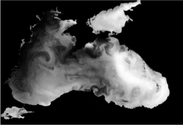
frequency of the satellite is at best one day. But, we usually have several acquisitions for the same day coming from different satel-lites using the same sensor. Figure 1 displays a SST image acquired in July 14th, 1998. These images present several artefacts such as:
(1) problems due to the geometry acquisition: unavailable infor-mation appearing as black and white spots,
(2) clouds: colder than the sea surface they appear darker on im-ages,
(3) problems due to sensor saturation: highly bright zones, (4) large spatial variation of the local temperature average, (5) high temporal variation of the global temperature average
be-tween acquisitions: due to solar exposition at the acquisition time and to different sensors calibration.
We need to construct a dedicated operator to estimate circulation velocity. The problem of motion estimation from image sequences
Fig. 1. SST image of the Black Sea given by NOAA/AVHRR.
has been extensively studied [5, 6, 7, 8, 9, 10, 11, 12, 13]. The clas-sical computer vision approach relies on a dense estimation of the displacement velocity based on the so-called conservation of gray level-value assumption (also called optical flow constraint): given a pixel (x(t), y(t)) on an image I at time t, we have:
dI
dt(x, y, t) = ∇I · w + ∂I
∂t = 0, (2)
where ∇I is the spatial gradient, w is the displacement between two consecutive images, and · denotes the scalar product. Equation (2) expresses the pixel’s luminance conservation over time: moving points keep a constant brightness during their motion. This equation has two unknowns: w = (u, v) and cannot be directly solved. One classical approach is to add an additional constraint, for example a
L2regularity for w, and to express it within an energy minimization
framework to obtain an estimation of w.
Due to their special artefacts, oceanographic satellite images must be preprocessed in order to use such kind of dense motion es-timation approaches. The section 2 presents the whole processing chain. Image preprocessing is presented in subsection 2.1. Subsec-tion 2.2 defines a moSubsec-tion estimator dedicated to the oceanographic application, ie: define conservation constraint and regularity equa-tion that we have to use and how do we solve the minimizaequa-tion prob-lem, in order to better adapt the operator to the specific context of acquisition process and observed phenomena. And subsection 2.3 presents the assimilation of estimated velocities into the circulation model. The section 3 presents different results with and without as-similation of estimated velocities, and compare them to results ob-tained using assimilation of other quantities. Finally section 4 gives conclusions and several perspectives to this work.
2. PROCESSING CHAIN 2.1. Image preprocessing
As we have seen in section 1, SST images coming from NOAA/AV-HRR present some artefacts able to compromise estimation of appar-ent motion with a dense estimator. We need to propose an adapted processing for each artefact.
Artefacts (1) no acquisition, (2) clouds, and (3) sensor saturation have to be masked. The mask is obtain by thresholding the original
image:
1. pixels not corresponding to an effective acquisition have ei-ther a temperature equal to 0oC or greater than 25oC;
2. clouds have a lower temperature than the ocean surface, pix-els with a temperature lower than 10oC are considered to be
clouds;
3. temperatures greater than 23oC are considered to be in the
saturation zone of the sensor.
Finally we keep in consideration only sea surface temperatures be-tween 10oC and 23oC, other pixels are masked and not taken into
account into the estimation process.
The correction of artefacts (4) and (5) corresponding to the high spatio-temporal variations of the temperature is crucial. It is directly linked to the evaluation of derivatives, mandatory step to solve dense motion estimation equations. To correct the high temporal varia-tion Vigan [14] proposed to apply a low-pass filter to ∂T /∂t in the Fourier domain. These kind of approach present the drawback to be difficult to tune because it assume a periodical aspect difficult to quantify. Moreover it begins difficult to deal with masks in the frequency domain. We have chosen to correct artefacts (4) in the spatial domain and then to correct artefacts (5): we consider large scale space phenomena to be extended at about 150km2, we
com-pute average temperature on 150 × 150km windows and subtract this average to the temperature of each pixel, it corrects the large spatial variation; once this correction done, we compute the global average for each image and deduce the mean bias for each couple of images, it corrects the high temporal variation.
2.2. Estimation of circulation velocities
In the context of fluid motion on oceanographic images, we are now able to keep the dense estimation framework and its energy mini-mization, but we need to further analyze the two components of the energy function to be minimized: conservation equation and regu-larity constraint, with respect the physical underlying process.
In order to investigate which conservation equation and regular-ity constraint are best adapted, we have used synthetic data coming from the 3D simulation model OPA [15] developed in the LOCEAN laboratory. We have shown in [16] that the best conservation equa-tion to estimate the moequa-tion is:
∇T · w +∂T
∂t = 0 (3)
ie: the gray level value conservation (2) applied to temperature. This
is coherent with the physical equation of the horizontal temperature transport, the horizontal diffusivity is negligible compared to the fre-quency of acquisition. But we have also seen in [16] that equation (3) is not respected everywhere. Actually, we have shown that there is two cases where the conservation equation isn’t verified: on specific oceanographic structures called filaments and when image informa-tion is not reliable (in the case of low spatial or temporal deriva-tives). We have designed an image based criteria to select points where we expect a rather good estimation according to the conserva-tion assumpconserva-tion. We obtain a selecconserva-tion of reliable points discarding both filaments (using a presegmentation process) and low informa-tion pixels (using thresholds on the moinforma-tion index Tt/∇T ).
In the same way, we have to choose which regularization criteria is the best adapted to the oceanographic context. By using synthetic data, we have shown that spatial regularity of the velocity norm L2
[10] or L1[9] are not well adapted to fluid motion. The best
crite-ria is based on the div/curl operators able to make the difference between irrotational and solenoidal components of the motion field:
min Z
img
αk∇divwk2+ βk∇curlwk2 (4)
where α and β are coefficients used to weight respectively the irrota-tional and solenoidal components. They are calibrated for this study in order to penalize the divergence according to uncompressible fluid properties.
In order to take into account the selection of reliable points and to avoid to handle 4th order PDE, the method we use to solve the minimization problem is based on spline vector field interpolation [17, 18]. The method tends to reconstruct a dense motion field from a set of observation corresponding to projection of motion vectors onto the image gradient. The vector field w is constrained to comply with the conservation equation on the reliable points riand to verify
the div/curl regularity on the whole image: 8 > > < > > : ∇T · w(ri) = − ∂T∂t (ri) i ∈ {1 . . . N }. min Z img αk∇divwk2+ βk∇curlwk2 (5)
The above system admits an unique solution, which can be deter-mined explicitly.
2.3. Assimilation of estimated velocities
Data assimilation is a global mathematical framework for combining data and mathematical model equations, in order to restore as best as possible the state variables of the model. Its principle consists of finding the analyze a of the state variable X according to observa-tions Xobs. Sequential data assimilation approaches, like Kalman
based methods compute the analyze as:
a = K[Xobs− HX] + X
where H stands for the observation operator and K is the Kalman matrix. In this study, we use a simplification of Kalman approaches, a nudging method, where the analyze is given by:
a = λ[Xobs− HX] + X,
the Kalman matrix is replaced by a constant coefficient λ a priori evaluated and called the nudging term.
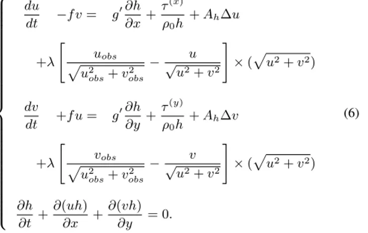
Using this nudging approach we can introduce the estimated ve-locity w = (uobs, vobs) into the system (1) such as:
8 > > > > > > > > > > > > > > > > > > > > > > > < > > > > > > > > > > > > > > > > > > > > > > > : du dt −f v = g 0∂h ∂x+ τ(x) ρ0h + Ah∆u +λ " uobs p u2 obs+ v2obs −√ u u2+ v2 # × (pu2+ v2) dv dt +f u = g 0∂h ∂y+ τ(y) ρ0h + Ah∆v +λ " vobs p u2 obs+ v2obs −√ v u2+ v2 # × (pu2+ v2) ∂h ∂t + ∂(uh) ∂x + ∂(vh) ∂y = 0. (6)
Note that in system (6) we have only take into account the orien-tation of the estimated velocity w. The estimated norm is not reliable enough. It explains why the velocity components are normalized in equations above.
3. RESULTS
In order to evaluate the result obtain with and without assimilation of the estimated velocity, we use another result obtain by the asim-ilation of the elevation of the sea surface. The sea surface elevation is directly linked to the thickness of the mixed layer state variable of the shallow-water model. This assimilation process has been dis-cribed in [4], it uses the same nudging approach as in system (6).
To quantify differences between two velocity fields w1and w2,
we use the angular error ψ = arccos(w1·w2) (expressed in degrees)
and the vorticity error ζ =p(curlw1− curlw2)2. Table 1 presents
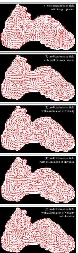
comparisons between the different results obtain for the same date. Figure 2 displays the different results without and with assimilation of the estimated velocity and sea surface elevation. Moreover, the last result (Fig.2 - plate 5) corresponds to velocity field obtain by coupling the assimilation of both velocity and elevation; for this ex-periment we used the same weight on velocity and elevation observa-tions. The use of assimilation allows a finer prediction of the veloc-ity: small relevant structures such as eddies are better described than on the predicted result without assimilation. On the other hand, the assimilation process tends to provide a physical certification to the velocity estimation result, in coherence with the prediction model. Finally, using assimilation of different kinds of observations is easy to set up in this application, mainly because observation operators correspond to projections. Predicted Motion Field Assimilation of Velocity Assimilation of Elevation Assimilation of Velocity and Elevation Estimated ψ 28.26 22.51 28.74 27.79 Motion Field ζ 1.41 1.16 1.42 1.38 Predicted ψ 22.4 15.76 19.99 Motion Field ζ 1.19 0.92 1.04 Assimilation ψ 22.09 19.06 of Velocity ζ 1.12 1.08 Assimilation ψ 13.45 Elevation ζ 0.79 Comparison between different results
Table 1. Comparison of velocity fields obtain with and without as-similation.
4. CONCLUSION AND PERSPECTIVES
In this study we have tackled the problem of data assimilation of in-formation coming from images into a simulation model. We have designed an image operator dedicated to SST images and oceano-graphic application in order to estimate dense velocity fields. The oceanographic circulation model used is a 2D shallow-water model. We have considered that the estimated apparent velocity was com-parable to the shallow-water velocity in order to use estimations as velocity observations. The assimilation method used is based on a nudging approach. In this framework we have demonstrate the po-tentialities of data assimilation methods.
We have two levels of perspectives for this work. The first level is the direct continuation of this study: we can enhance both the velocity estimator (by adding new a priori information) and the as-similation method (better estimation of the nudging term or use of Kalman approaches). The second level is a general perspective for
(1) estimated motion field with image operator
(2) predicted motion field with shallow−water model
(3) predicted motion field with assimilation of velocity
with assimilation of elevation (4) predicted motion field
(5) predicted motion field with assimilation of velocity and elevation
Fig. 2. Different results with and without assimilation.
image data assimilation: we should assimilate other kind of struc-tures coming from oceanographic images, such as eddies, fronts, fil-aments, etc.
5. REFERENCES
[1] R. Stewart, Introduction to Physical Oceanography, Depart-ment of Oceanography, Texas A&M University, 2002. [2] E. Blayo, “Modélisation numérique et assimilation de données
en océanographie - Habilitation à Diriger des Recherches,” 2002.
[3] B. de Saint-Venant, “Théorie du movement non-permanent des eaux,” Compte-Rendu de l’Académie des Sciences, Paris, 1871.
[4] G. Korotaev, T. Oguz, A. Nikiforov, and C. Koblinsky, “Sea-sonal, interanual, and mesoscale variability of the Black Sea upper layer circulation derived from altimeter data,” Journal
of Geophysical Research, vol. 108, no. C4, 3122, 2003.
[5] L. Alvarez, J. Weickert, and J. Sanchez, “Reliable estimation of dense optical flow fields with large displacements,” IJCV, vol. 39, no. 1, pp. 41–56, August 2000.
[6] J. Barron, D. Fleet, and S. Beauchemin, “Performance of op-tical flow techniques,” International Journal of Computer
Vi-sion, vol. 12, no. 1, pp. 43–77, 1994.
[7] S.S. Beauchemin and J.L. Barron, “The computation of optical flow,” Surveys, vol. 27, no. 3, pp. 433–467, September 1995. [8] D. Béréziat, I. Herlin, and L. Younes, “A generalized optical
flow constraint and its physical interpretation,” in Proceedings
of CVPR’2000, 2000.
[9] I. Cohen and I. Herlin, “Optical flow and phase portrait meth-ods for environmental satellite image sequences,” in ECCV, 1996, vol. 2, p. 141.
[10] B.K.P. Horn and B.G. Schunk, “Determining optical flow,”
Artificial Intelligence, vol. Vol 17, pp. 185–203, 1981.
[11] A. Mitiche and P. Bouthemy, “Computation and analysis of image motion: A synopsis of current problems and methods,”
International Journal of Computer Vision, vol. Vol 19, no. 1,
pp. 29–55, 1996.
[12] H.H. Nagel, “Displacement vectors derived from second-order intensity variations in image sequences,” Computer Graphics
Image Processing, vol. 21, pp. 85–117, 1983.
[13] R.P. Wildes and M.J. Amabile, “Physically based fluid flow recovery from image sequences,” in CVPR97, 1997, pp. 969– 975.
[14] X. Vigan, C. Provost, R. Bleck, and P. Courtier, “Sea surface velocities from Sea Surface Temperature image sequences,”
Journal of Geophysical Research, August 2000.
[15] G. Madec, M. Imbard, and C. Lévy, OPA 8.1 Ocean General
Circulation Model Reference Manual, Institut Pierre Simon
Laplace, Paris, 1999, Notes scientifiques du pôle modélisation. [16] I. Herlin, F. X. Le Dimet, E. Huot, and J. P. Berroir, Coupling
models and data: which possibilities for remotely-sensed im-ages?, chapter e-Environement: progress and challenges, pp.
365–383, Instituto Politécnico Nacional, México, 2004. [17] L. Amodei, “A vector spline approximation,” Journal of
ap-proximation theory, vol. 67, pp. 51–79, 1991.
[18] D. Suter, “Motion estimation and vector splines,” in CVPR94, 1994.