HAL Id: hal-00317185
https://hal.archives-ouvertes.fr/hal-00317185
Submitted on 1 Jan 2002
HAL is a multi-disciplinary open access
archive for the deposit and dissemination of
sci-entific research documents, whether they are
pub-lished or not. The documents may come from
teaching and research institutions in France or
abroad, or from public or private research centers.
L’archive ouverte pluridisciplinaire HAL, est
destinée au dépôt et à la diffusion de documents
scientifiques de niveau recherche, publiés ou non,
émanant des établissements d’enseignement et de
recherche français ou étrangers, des laboratoires
publics ou privés.
A. V. Mikhailov, D. Marin, T. Yu. Leschinskaya, M. Herraiz
To cite this version:
A. V. Mikhailov, D. Marin, T. Yu. Leschinskaya, M. Herraiz. A revised approach to the ?oF2
long-term trends analysis. Annales Geophysicae, European Geosciences Union, 2002, 20 (10), pp.1663-1675.
�hal-00317185�
Annales
Geophysicae
A revised approach to the foF2 long-term trends analysis
A. V. Mikhailov1, D. Marin2, T. Yu. Leschinskaya1, and M. Herraiz3
1Institute of Terrestrial Magnetism, Ionosphere and Radio Wave Propagation, Troitsk, Moscow Region 142190, Russia 2Atmospheric Sounding Station “El Arenosillo”, INTA, Spain
3Faculty of Physics, Complutense University, Spain
Received: 14 March 2001 – Revised: 4 February 2002 – Accepted: 6 February 2002
Abstract. A new approach to extract foF2 long-term trends, which are free to a great extent from solar and geomagnetic activity effects, has been proposed. These trends are insensi-tive to the phase (increasing/decreasing) of geomagnetic ac-tivity, with long-term variations being small and insignificant for such relatively short time periods. A small but significant residual foF2 trend, with the slope Kr = −2.2 × 10⁻⁴per
year, was obtained over a 55-year period (the longest avail-able) of observations at Slough. Such small trends have no practical importance. On the other hand, negative (although insignificant) residual trends obtained at 10 ionosonde sta-tions for shorter periods (31 years) may be considered as a manifestation of a very long-term geomagnetic activity in-crease which did take place during the 20th century. All of the revealed foF2 long-term variations (trends) are shown to have a natural origin related to long-term variations in so-lar and geomagnetic activity. There is no indication of any manmade foF2 trends.
Key words. Ionosphere (ionosphere-atmosphere interac-tions, ionospheric disturbances)
1 Introduction
Due to an increasing interest in the anthropogenic impact on the Earth’s atmosphere the ionospheric parameter long-term trends are widely discussed in recent publications (Bre-mer, 1992, 1998; Givishvili and Leshchenko, 1994, 1995; Givishvili et al., 1995; Danilov, 1997, 1998; Ulich and Tu-runen, 1997; Rishbeth, 1997; Jarvis et al., 1998; Upadhyay and Mahajan, 1998; Sharma et al., 1999; Foppiano et al., 1999; Danilov and Mikhailov, 1999; Mikhailov and Marin, 2000; Deminov et al., 2000; Danilov and Mikhailov, 2001). The interest in the ionospheric trend analysis was greatly stimulated by the model calculations of Rishbeth (1990) and Rishbeth and Roble (1992), who predicted the ionospheric effects of the atmosphere greenhouse gas concentration
in-Correspondence to: A. V. Mikhailov (avm71@orc.ru)
crease. Since then, researchers have been trying to reveal the predicted ionospheric effects related to the thermosphere cooling (Bremer, 1992; Givishvili and Leshchenko, 1994; Ulich and Turunen, 1997, Jarvis et al., 1998; Upadhyay and Mahajan, 1998). The atmosphere cooling effect should have been noticeable in the hmF2 rather than in the foF2 trends, due to a weak dependence of NmF2 on neutral temperature. Moreover, the expected neutral temperature decrease due to the greenhouse effect should result in a positive foF2 trend in contrast to the observations (Mikhailov and Marin, 2000). The analyzes have shown that there are well-pronounced and significant hmF2 as well as foF2 trends. The worldwide pat-tern of the F2-layer parameter trends turned out to be very complicated and this cannot be reconciled with the green-house hypothesis. On the other hand, one cannot exclude the anthropogenic effects in the upper atmosphere related to the increasing rate of rocket and satellite launching during the last few decades, which has led to the thermosphere pollu-tion (Kozlov and Smirnova, 1999; Adushkin et al., 2000). Therefore, further efforts are required in this direction to find out the physical mechanism of the F2-layer trends.
Despite many publications devoted to the F2-layer param-eter long-term trends, the results of different authors are still contradictory to a great extent. This is due to both the ac-curacy of the experimental material and the methods used to extract long-term trends from the observations. The most suitable for the trend analysis parameter is the F2-layer criti-cal frequency. It has been observed routinely over the world-wide ionosonde network for 3–5 solar cycles using one and the same method of ionospheric sounding. The critical fre-quency, foF2, is registered directly (unlike hmF2) and with an acceptable accuracy of ≈ 0.1 MHz. Unlike foE or foF1, the F2-layer critical frequency is observed all day long and this allows one to follow diurnal variations in the foF2 long-term trends. But even in case of foF2, the useful “signal” is very small and the “background” is very noisy, therefore, the success of analysis depends strongly on the method used. An approach being developed by Danilov and Mikhailov (1999) and Mikhailov and Marin (2000, 2001) has allowed us to
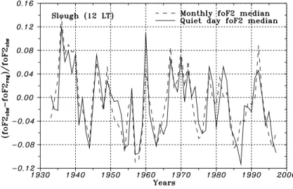
Fig. 1. A comparison of annual mean δfoF2 variations at Slough (12:00 LT)
when the usual monthly median and Q-median foF2 values are used in the cal-culations.
find systematic variations in foF2 and hmF2 trends, unlike other approaches (e.g. Bremer, 1998; Upadhyay and Maha-jan, 1998), resulting in various signs and magnitudes of the trends at various stations. An application of this approach to the foF2 trend analysis resulted in a geomagnetic control concept (Mikhailov and Marin, 2000, 2001) to explain the revealed latitudinal and diurnal variations of the F2-layer pa-rameter long-term trends. It was shown that an interpretation of the F2-layer parameter trends should consider the geomag-netic effects as an inalienable part of the trends revealed and this can be done based on the contemporary understanding of the F2-layer storm mechanisms (Mikhailov and Marin, 2000, 2001).
Although the geomagnetic control concept allowed us to explain the main morphological features of the foF2 long-term trends revealed, there are still some questions remain-ing. The most important one is whether it is possible to re-move the geomagnetic effect from the foF2 long-term vari-ations, in order to analyze the residual trends. What is the origin (anthropogenic or natural) of such residual trends if they exist? Earlier developed approaches cannot be used for such analysis as they give foF2 trends that are strongly con-taminated with geomagnetic activity effects, despite the at-tempts to delete them (Mikhailov and Marin, 2000, 2001). Therefore, a revised method has been developed in this pa-per which allows us to delete to a great extent solar and ge-omagnetic activity effects from the observed foF2 long-term variations and reveal the residual foF2 trends.
2 Method description
A revised method described here is based on the analysis given in Sect. 3 of the paper. The final version of the method comprises the following.
1. We proceed from an assumption that observed foF2 variations are mainly due to solar and long-term ge-omagnetic activity variations that (with some reserva-tions) may be described with R12 and 11-year running
mean Ap indices. The results of our analysis (see later) have shown that such a combination provides the best description accuracy and the most consistent results. Therefore, the method includes the following steps. A regression of monthly foF2 with R12
foF 2reg =a0+a1Rα12 (1)
is used to find monthly relative deviations
δfoF 2 = (foF 2obs−foF 2reg)/foF 2obs. (2)
We analyze (for each LT moment) relative rather than absolute δfoF2 deviations considered in the foF2 and
hmF2 trend analyzes by Bremer (1998); Ulich and Tu-runen (1997); Jarvis et al. (1998); Upadhyay and Maha-jan (1998); Sharma et al. (1999); Foppiano et al. (1999). As far as we know relative deviations were considered only by Deminov et al. (2000) in their foF2 long-term trend analysis. Relative deviations allow us to com-bine different months and obtain an annual mean δfoF2 that is used in the analysis, with the final method be-ing based on the 11-year runnbe-ing mean δfoF2 values. A simple arithmetic running mean smoothing with an 11-year gate is applied everywhere.
The optimal 12 different values of α (for each month of the year) are specified to provide the least standard de-viation (SD) after a regression (see later) of an 11-year smoothed δfoF2 with Ap132(11-year running mean Ap
indices). The 11-year δfoF2 smoothing requires all 12 values of α to be available simultaneously at each step of the SD minimization. This implies an application of special multi-regressional methods (Press et al., 1992) matched to solve the problem considered.
The expression (1) is of a general type and depending on α, it can describe both the linear and nonlinear rela-tionship of foF2 with R12. The regression coefficients
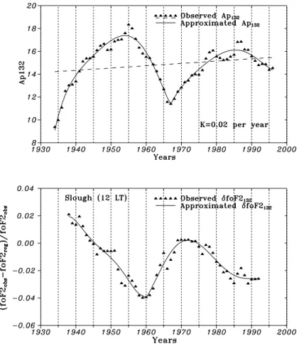
Fig. 2. Observed and polynomial
ap-proximated Ap132and δfoF2132
varia-tions used in the trend analysis. Dashed line is a linear, very long-term trend with the slope K = 0.02 per year in geomagnetic activity obtained over the observed Ap132 variations. Note also
a 4-year shift between the Ap132 and
δfoF2132variations.
month and a given α value. It should be stressed that the expression (1) does not provide the best approxima-tion of the observed foF2 versus R12dependence (other
dependencies may yield a smaller sum of the residu-als), but it should be considered in terms of the follow-ing regression with Ap132to find the minimal SD (see
later). Therefore, the regression (1) is not a “model” in the usual sense of the word, since it is accepted in all earlier approaches. This regression is used to remove the solar activity part from the observed foF2 variations as a “pure” foF2 dependence on solar activity (presented by the R12index) a priori is not known for each month
(see Sect. 6: Discussion).
2. Q-medians proposed by Deminov et al. (2000) are used in the method instead of the usual monthly foF2 ones. Such Q-medians are obtained over quiet days of each month. In our approach, unlike that of Deminov et al. (2000), a day is considered to be quiet if daily Ap ≤ 10 for this and the two previous days. The Q-median value is set to zero if there are no such days in a month. A threshold was set to 1 and 3 quiet days a month. Testing has shown that generally 3-quiet day medians provide better results for some stations, but too many gaps in the observations, due to such severe selection, led to pe-culiar results on other stations. Therefore, the 1-quiet day threshold has been accepted. An example of annual
mean δfoF2 (after Eq. 2) variations obtained with the usual monthly and Q-medians is shown in Fig. 1. The difference is seen for the two cases, both during the pe-riods of solar maximum and minimum. It may seem not to be very large, but one should keep in mind that during the trend analysis, we work at the level of noise and even small differences in the initial material may affect the fi-nal result. Despite the removal of short-term (monthly) geomagnetic effects by using Q-medians, strong year-to-year δfoF2 fluctuations take place (Fig. 1). These os-cillations may be related to the variations in solar ac-tivity (Kholodny and Chertoprud, 1992; Ivanov-Kholodny, 2000), but they are not removed by any re-gression with R12or Ap, and an 11-year running mean
smoothing is applied to conquer them (see later).
3. Unlike our earlier method, where only years around so-lar cycle maxima and minima were analyzed to avoid the hysteresis effect at the rising and falling parts of so-lar cycles, the proposed method uses all years available. A comparison has shown close results for different year selections using the proposed method. This takes away the problem of using different year selections for foF2 and hmF2 trend analysis (Marin et al., 2001; Mikhailov and Marin, 2001).
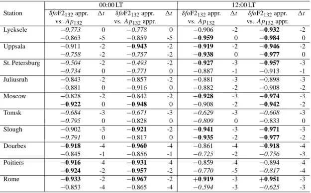
Table 1. Correlation coefficients, r, between δfoF2132 and Ap132found over one and the same period 1957–97 (1962–92 after 11-year
smoothing). The “appr.” refers to the polynomial approximated δfoF2132 and Ap132 variations. The first line refers to Q-medians, the
second to the usual monthly foF2 medians used in the calculations. Bold face figures show significant r with a confidence level 99%, normal face figures correspond to 95% confidence level, italic figures are not significant r. The optimal time shift 1t (in years) between δfoF2132
and Ap132variations is given as well
00:00 LT 12:00 LT
Station δfoF2132appr. 1t δfoF2132appr. 1t δfoF2132appr. 1t δfoF2132appr. 1t
vs. Ap132 vs. Ap132appr. vs. Ap132 vs. Ap132appr. Lycksele −0.773 0 −0.778 0 −0.906 -2 −0.932 -2 −0.863 -5 −0.859 -5 −0.959 0 −0.984 0 Uppsala −0.911 -2 −0.943 -2 −0.919 -2 −0.946 -2 −0.758 -2 −0.757 -2 −0.938 0 −0.977 0 St. Petersburg −0.504 -2 −0.493 -2 −0.927 -3 −0.957 -3 −0.734 0 −0.771 0 −0.887 -1 −0.913 -1 Juliusruh −0.843 -2 −0.857 -2 −0.881 -3 −0.898 -3 −0.881 0 −0.916 0 −0.882 -2 −0.908 -2 Moscow −0.828 -2 −0.842 -2 −0.928 -3 −0.974 -3 −0.922 0 −0.948 0 −0.908 -2 −0.942 -2 Tomsk −0.684 -3 −0.671 -3 −0.629 -3 −0.608 -3 −0.795 0 −0.828 0 −0.809 0 −0.833 0 Slough −0.902 -3 −0.921 -2 −0.941 -3 −0.971 -3 −0.791 0 −0.817 0 −0.935 -2 −0.977 -2 Dourbes −0.918 -4 −0.960 -4 −0.861 -4 −0.918 -4 −0.845 -1 −0.856 -1 −0.725 -2 −0.756 -3 Poitiers −0.916 -4 −0.931 -4 −0.859 -4 −0.894 -4 −0.924 -2 −0.957 -2 −0.770 -5 −0.817 -4 Rome −0.933 -2 −0.967 -2 +0.919 -3 +0.951 -3 −0.853 -4 −0.865 -4 −0.594 -3 −0.625 -3
of months with available foF2 values for a given year is less than 6, then the year is marked as “zero”. Dur-ing the 11-year δfoF2 smoothDur-ing, the arithmetic mean is calculated over the non-zero years only.
4. The geomagnetic activity effect is deleted from the 11-year running mean δfoF2 variation using a regression with Ap132
δfoF 2132=b0+b1Ap132(t + n)
+b2Ap2132(t + n) , (3)
where n is a time shift in years of Ap132with respect to
δfoF2132 variations, which is selected to give the least
SDfor the residuals after Eq. (3). The regression co-efficients bi are specified by the least-squares method.
A nonlinear dependence of δfoF2 on the geomagnetic activity is expected in accordance with Zevakina and Kiseleva (1978) and Muhtarov and Kutiev (1998).
5. An analysis has shown that the best results (the least
SD) can be obtained if an additional smoothing is ap-plied to δfoF2132 and Ap132 variations. Such
smooth-ing is made by a 5-order polynomial approximation of these parameter variations. The initial and approxi-mated Ap132and δfoF2132variations are shown in Fig. 2
for Slough (12:00 LT) as an example. A 4-year shift is clearly seen between the two variations.
6. The residual linear trend with the slope Kr (in 10−4
per year) is estimated over the residuals after the regres-sion (3).
7. The test of significance for the linear trend parameter
Kr(the slope), as well as for the correlation between the
parameters analyzed, is made with Fisher’s F criterion (Pollard, 1977)
F = r2(N −2)/(1 − r2) ,
where r is the correlation coefficient and N is the num-ber of pairs considered. Keeping in mind that we work with smoothed variations we set the number of degrees of freedom to be (N − 2) = 4 (the 5th order polynomial is defined by 6 coefficients). Such tough requirements on the (N − 2) value formally results in insignificant trends, in many cases, despite the existence of obvious and pronounced trends calculated over some dozens of points. Sometimes the number of degrees of freedom is higher than 4 and this is mentioned separately in each case. Student’s T-criterion (Pollard,1977) was used to test whether the difference between values is significant.
3 Choosing a combination of parameters
In developing the method we have considered monthly, the annual mean and the 11-year running mean δfoF2, to find the
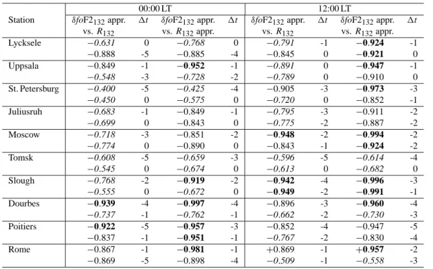
Table 2. Correlation coefficients, r, between δfoF2132 and R132 found over one and the same period 1957–97 (1962–92 after 11-year
smoothing). The “appr.” refers to the polynomial approximated δfoF2132and R132variations. The first line refers to Q-medians, the second
to the usual monthly foF2 medians used in the calculations. Bold face figures show significant r with a confidence level 99%, normal face figures correspond to 95% confidence level, italic figures are not significant r. The optimal time shift 1t (in years) between δfoF2132and
R132variations is given as well
00:00 LT 12:00 LT
Station δfoF2132appr. 1t δfoF2132appr. 1t δfoF2132appr. 1t δfoF2132appr. 1t
vs. R132 vs. R132appr. vs. R132 vs. R132appr. Lycksele −0.631 0 −0.768 0 −0.791 -1 −0.924 -1 −0.888 -5 −0.885 -4 −0.845 0 −0.921 0 Uppsala −0.849 -1 −0.952 -1 −0.891 0 −0.947 -1 −0.548 -3 −0.728 -2 −0.789 0 −0.910 0 St. Petersburg −0.400 -5 −0.425 -4 −0.905 -3 −0.973 -3 −0.450 0 −0.575 0 −0.720 0 −0.852 -1 Juliusruh −0.683 -1 −0.849 -1 −0.795 -3 −0.911 -2 −0.699 0 −0.843 0 −0.775 -2 −0.887 -2 Moscow −0.718 -3 −0.851 -2 −0.948 -2 −0.994 -2 −0.774 0 −0.890 0 −0.843 -1 −0.924 -2 Tomsk −0.608 -5 −0.659 -3 −0.596 -5 −0.614 -4 −0.545 0 −0.674 0 −0.613 0 −0.682 0 Slough −0.768 -2 −0.919 -2 −0.942 -4 −0.996 -3 −0.555 0 −0.672 0 −0.949 -2 −0.991 -1 Dourbes −0.939 -4 −0.997 -4 −0.896 -3 −0.960 -4 −0.737 -1 −0.762 -1 −0.662 -2 −0.730 -3 Poitiers −0.922 -5 −0.957 -3 −0.852 -4 −0.947 -5 −0.837 -1 −0.951 -1 −0.767 -2 −0.830 -4 Rome −0.867 -1 −0.981 -1 +0.869 -1 +0.957 -2 −0.869 -5 −0.898 -4 −0.509 -1 −0.558 -3
combination which would provide the least SD after delet-ing the geomagnetic activity effect. The latter was supposed to be presented by smoothed or non-smoothed Ap or R12
indices. Usual monthly and Q-median, smoothed and non-smoothed foF2 values were considered. The R12 index was
considered (along with Ap) as an indicator of long-term so-lar/geomagnetic activity variations (Deminov et al., 2000). In the beginning we examined the correlation coefficients be-tween δfoF2 and Ap (or R12) indices. Only the results which
led us to the final method (Sect. 2) are presented here. All correlation coefficients for monthly, as well as for an-nual mean δfoF2, are found to be low (0.2–0.5), both for non-smoothed and non-smoothed Ap (or R12) indices and, therefore,
cannot be considered as candidates for the method. An es-sential increase in the correlation coefficient takes place only after moving to 11-year running mean values. An additional increase in the correlation is possible if one applies a smooth-ing approximation to δfoF2132and Ap132(or R132) variations
(Fig. 2). Such approximated values provide the largest corre-lation coefficients and the least SD; therefore, this approach was used in the final method.
The testing results over 10 stations are given in Tables 1 and 2, where Q- and the usual monthly foF2 medians are compared. Ap132and Ap132approximated indices were used
in Table 1, while R132and R132approximated – in Table 2.
One and the same period 1957–1997 (1962–1992 after the 11-year smoothing) for all stations was considered.
Max-imal correlation coefficients corresponding to the optMax-imal time shift of Ap132(or R132), with respect to δfoF2132
varia-tions, are given in Tables 1 and 2 for 00:00 and 12:00 LT. The results of Tables 1 and 2 show that the correlation co-efficients are larger when both approximated δfoF2132 and
Ap132 (or R132) variations are considered. The difference
when approximated and non-approximated indices are used is significant at the 99.9% confidence level according to the T-criterion. The use of Q-medians compared to the usual monthly ones provides a larger number of significant cases. The percentage of significant cases (Q-medians/usual medi-ans) is 80% / 67% when Ap132is used, and 67% / 45% when
R132is considered. Therefore, Q-medians seem to be
prefer-able for the method. On the other hand, the difference be-tween significant correlation coefficients from Tables 1 and 2 is not significant according to the T-criterion when Ap132
is used, and the difference between the two medians is sig-nificant at the 98% confidence level (Q-medians are better) when R132is considered. Thus, some additional
character-istics should be compared. A comparison of the time shift between δfoF2 and Ap132 (or R132) variations can help
se-lect the best combination. The average optimal time shifts along with SD calculated for the significant cases from Ta-bles 1 and 2 are given in Table 3. The Q-medians/Ap132
ap-proximated combination provides the least SD for the time shift, which is around −3 years. This combination has been chosen for the final method.
Table 3. Average optimal time shift with ±SD between δfoF2 and Ap132(or R132) approximated variations calculated from the results of
Tables 1 and 2
Q-medians Usual monthly medians
Ap132appr. R132appr. Ap132appr. R132appr.
−2.8±0.83 −2.3±1.25 −1.4±1.59 −1.6±1.62
Table 4. Ionosonde stations and calculated slope Kr(in 10−4per year) for the period of increasing geomagnetic activity 1965–1991. KM+m
values from Mikhailov and Marin (2000) are given for a comparison. Bold face figures for KM+mshow significant trends with a confidence
level ≥ 90%, italic face figures are trends which are not significant at the 90% confidence level
Station 8 8inv Geographic 00:00 LT 12:00 LT
Deg Deg Lat Lon Kr KM+m Kr KM+m
Lycksele 62.70 61.42 64.70 18.80 −6.21 +1.9 −0.96 −26.0 Uppsala 58.44 56.61 59.80 17.60 −0.56 −42.2 −0.40 −27.6 St. Petersburg 56.17 55.91 60.00 30.70 −1.04 −19.2 −0.09 −16.1 Juliusruh 54.40 51.61 54.60 13.40 −1.80 −33.7 −0.82 −12.2 Ekateringburg 48.42 51.45 56.70 61.10 −5.20 −30.2 −0.31 −12.0 Moscow 50.82 51.06 55.50 37.30 −1.10 −25.6 +0.31 −12.0 Tomsk 45.92 50.58 56.50 84.90 −0.95 −16.9 −1.10 +5.0 Slough 54.25 49.80 51.50 359.43 −0.27 −13.1 −0.52 −5.9 Dourbes 51.89 47.80 50.10 4.60 −0.30 −3.9 −0.25 +1.7 Poitiers 49.40 45.05 46.60 0.30 −0.83 −9.4 −0.67 −0.3 Rome 42.46 37.48 41.90 12.52 0.00 −2.3 −2.57 +6.2 Ashkhabad 30.39 30.55 37.90 58.30 −0.40 −4.4 −0.88 −1.4
Table 5. Same as Table 4, but for the period of decreasing geomagnetic activity 1955–1970
Station 00:00 LT 12:00 LT
Kr KM+m Kr KM+m
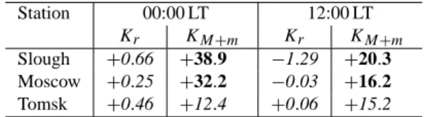
Slough +0.66 +38.9 −1.29 +20.3
Moscow +0.25 +32.2 −0.03 +16.2
Tomsk +0.46 +12.4 +0.06 +15.2
The obtained significant correlation coefficients (Tables 1 and 2) are seen to be large and negative both for 00:00 and 12:00 LT. The only case of positive correlation of δfoF2 with geomagnetic activity is demonstrated at the lower latitude station of Rome at 12:00 LT, and this may be explained in the framework of contemporary F2-layer storm mechanisms (Mikhailov and Marin, 2001).
4 Rising and falling periods in geomagnetic activity The basic points of the geomagnetic control concept by Mikhailov and Marin (2000) is the dependence of foF2 trends on geomagnetic (invariant) latitude and the existence of negative/positive foF2 trends for the periods of long-term increasing/decreasing geomagnetic activity. Both fea-tures were explained using the F2-layer storm mechanisms (Mikhailov and Marin, 2001). Therefore, if the revised ap-proach is free of the geomagnetic control, then both features
should be absent in the foF2 trends revealed. The same pe-riod 1965–1991, as in Mikhailov and Marin (2000) of in-creasing geomagnetic activity (Fig. 2, top), was chosen for the analysis (Table 4). Keeping in mind the 11-year smooth-ing, only stations with available observations for the period 1960–1996 could be analyzed. Slopes K for (M+m) year selection from Mikhailov and Marin (2000) are given for a comparison. Table 4 shows that unlike our previous re-sults the calculated trends do not demonstrate any latitudi-nal dependence being small and insignificant. Relatively large and insignificant Krfor Lycksele (00:00 LT) and Rome
(12:00 LT) are random and due to the scatter of data for the conditions in question.
Similar analysis was made for the 1955–1970 period (Ta-ble 5) of decreasing geomagnetic activity (Fig. 2, top) for the 3 stations from Mikhailov and Marin (2000) where ob-servations are available at least since 1950. The calculated trends are seen to be small and insignificant, while KM+m
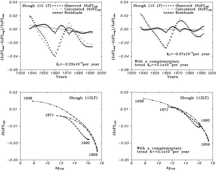
Fig. 3. Observed, calculated δfoF2132and their difference resulting in a residual foF2 trend with the slope Kr for Slough 12:00 LT (top
panels), along with the relationship between polynomial approximated δfoF2132and Ap132(bottom panels). Right-hand panels show the results with a complementary trend (Kc = +3.1 × 10⁻⁴per year). Note the tightening of two branches in the δfoF2132versus Ap132
dependence (left-hand, bottom) after applying a complementary trend (right-hand, bottom).
are large and positive, in accordance with the geomagnetic control concept.
The results obtained show that the proposed method pro-vides foF2 trends which are small, insignificant and latitudi-nal independent, regardless of the phase of the geomagnetic activity long-term variation. This means that trends are free of geomagnetic effects in terms of the geomagnetic control concept. On the other hand, most of the trends are seen to be negative (Table 4) and this may tell us about an additional mechanism affecting the trends (see later).
5 Residual foF2 trends
The obtained foF2 trends were shown to be insignificant for relatively short time intervals (rising or falling periods of ge-omagnetic activity). Obviously, high correlation coefficients, resulting in good fitting and small Kr, can be easier obtained
for short time intervals, including only one branch of the ge-omagnetic activity variation, but this may not be the case for longer periods. Therefore, the method was applied to Slough where foF2 observations for 12:00 LT are available for the 1933–1997 period. After 11-year smoothing, the available period for analysis reduces to 1938–1992. Calculated and observed δfoF2132variations, as well as their differences, are
shown in Fig. 3 (left-hand, top). The proposed method is seen to describe the main features of the observed δfoF2132
varia-tion. The residuals demonstrate a long-term linear trend with a slope Kr = −2.23 × 10⁻⁴per year, which is significant
at the 95% confidence level. Instead of pronounced negative
foF2 trends for the 1940–1960 and 1970–1992 periods and
a positive trend for the 1960–1970 period, which we would have under the geomagnetic control concept, the residuals (Fig. 3) do not reflect these long-term variations in geomag-netic activity. Some fluctuations of the residuals around the regression line reflect the imperfection of the model fitting
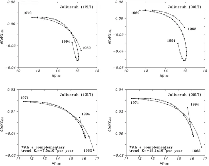
Fig. 4. Relationship between polynomial approximated δfoF2132and Ap132for Juliusruh (12:00 and 00:00 LT) (top panels) and the same
dependencies after applying a complementary trend (bottom). Note the tightening of the loops in the second case.
the observed δfoF2132variations.
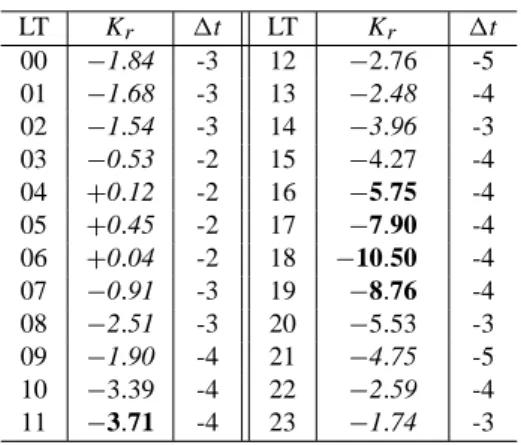
Strong diurnal variation of the foF2 trend magnitude was another feature revealed and explained in the framework of the geomagnetic control concept (Mikhailov and Marin, 2000, 2001). This was also checked for Slough where foF2 observations for all LT moments are available for the 1944– 1997 period. The results of the calculations are given in Ta-ble 6. Unlike our previous results, the calculated Krare small
and most of them are insignificant all day long. Only trends around noon and in the evening turn out to be significant. De-spite this insignificance in the trends (which were calculated absolutely independently for 24 LT moments), they clearly demonstrate a consistent pattern of some diurnal variation (Table 6). This means that the calculated trends are not ran-dom and may need physical interpretation in future. The im-portant result for further discussion is that most of the trends in Table 6 are negative similar to the conclusion made in Ta-ble 4. The optimal time shift between Ap132 and δfoF2132
variations averaged over 24 LT moments is −3.4±0.88 years.
This is comparable with the estimate obtained over 10 sta-tions for 12 LT (Table 3, the Q-medians/Ap132approximated
combination).
The residual trend is seen to result from incomplete fit-ting of the calculated δfoF2132variation to the observed one
(Fig. 3, left-hand, top). This is due to the δfoF2132 versus
Ap132regression used in the calculations. The left-hand
bot-tom panel of Fig. 3 gives a dependence between approxi-mated δfoF2132 and Ap132 values used in the calculations.
Two branches are seen in this dependence: one – before the end of the 1950s, the other – after 1971. The type of de-pendence is about the same, but the curves are seen to be shifted. An additional analysis has shown that the differ-ence between the two branches remains, regardless of the shift (−5 ÷ 0 years) applied to the Ap132variation with
re-spect to the δfoF2132one. It seems as if the “efficiency” of
geomagnetic disturbances has increased since the middle of the 1960s as the same δfoF2132 values correspond to lower
Table 6. Diurnal variation of the slope Kr (in 10−4per year) of the residual trend for Slough. The optimal time shift 1t (in years) between δfoF2132and Ap132variations is given as well. Bold face
figures show significant trends with a confidence level 95%, nor-mal face figures are trends with a confidence level 90%, italic face figures are trends which are not significant at the 90% confidence level LT Kr 1t LT Kr 1t 00 −1.84 -3 12 −2.76 -5 01 −1.68 -3 13 −2.48 -4 02 −1.54 -3 14 −3.96 -3 03 −0.53 -2 15 −4.27 -4 04 +0.12 -2 16 −5.75 -4 05 +0.45 -2 17 −7.90 -4 06 +0.04 -2 18 −10.50 -4 07 −0.91 -3 19 −8.76 -4 08 −2.51 -3 20 −5.53 -3 09 −1.90 -4 21 −4.75 -5 10 −3.39 -4 22 −2.59 -4 11 −3.71 -4 23 −1.74 -3
Table 7. The minimal SD (in 10−3) and corresponding slopes (in 10−4per year) of a complementary Kcand residual Kr trends for
Slough (12:00 LT). The start years for the complementary trend to start are shown
Start years SD Kc Kr 1980 4.19 +2.98 −1.79 1975 3.85 +3.22 −1.48 1970 3.38 +3.41 −1.18 1965 3.18 +3.04 −1.04 1960 2.88 +3.20 −0.73 1955 2.46 +3.19 −0.44 1950 2.14 +3.17 −0.18 1945 2.09 +3.27 −0.33 1940 1.99 +3.23 −0.23 1938 2.01 +3.11 −0.07
The ambiguity in this dependence can be removed to a great extent by applying a “complementary” linear trend to the δfoF2132variation. Table 7 shows the results of such
cal-culations for Slough (12:00 LT) when a complementary trend with the slope Kc was switched on for different start years.
The results of Table 7 show that SD and the slope Kr of
the residual trend decrease as the start year for the comple-mentary trend shifts towards the beginning of the period in question, with the complementary trend being about the same with the slope Kc, close to +3 × 10⁻⁴per year. The least SD
(the best fitting) is obtained if the complementary trend is applied for the whole period analyzed, starting from the first year, with the latter being important for further discussion. The final variations are shown in Fig. 3 (right-hand boxes). A complementary positive trend with Kc=3.1×10⁻⁴per year
tightens the loops in the δfoF2132 versus Ap132 dependence
to practically one curve (Fig. 3, right-hand, bottom). The re-sultant residual trend is close to zero (Kr = −0.07 × 10⁻⁴
per year) in this case. Similar results were obtained for some other stations with the complementary trends depending on station and LT. An example of tightening the loops in the
δfoF2132 versus Ap132 dependence demonstrates Juliusruh
for the 1962–1994 period (Fig. 4).
6 Discussion
The proposed approach to the foF2 trend analysis allows us to remove to a great extent solar and geomagnetic activity effects from foF2 long-term variations and to show that the residual foF2 trends are small both for rising and falling pe-riods of geomagnetic activity (Tables 4 and 5). The residual significant foF2 trend for Slough (12:00 LT), with the longest available period of foF2 observations, was found to be small with the slope Kr = −2.23 × 10⁻⁴per year. Such a small
trend gives around 0.1 MHz in the foF2 change over a 55-year period for any reasonable mean foF2 value accepted. Therefore, such trends have no practical importance. But from a physical point of view, the obtained result is inter-esting, telling us that practically all observed foF2 long-term variations may be attributed to the variations in solar and ge-omagnetic activity, i.e. they are of a natural origin. Although this result was obtained using conventional indices, R12and
Ap, they should be converted to Rα12and Ap132, to be used in
the trend analysis. This is due to the fact that initial R12and
monthly Ap cannot properly present solar and geomagnetic activity effects in the foF2 long-term variations and more ef-ficient indices are required. There are some related problems. The first one concerns the procedure of the solar activity ef-fect removal. The commonly accepted approach is based on the foF2 regression (linear dependence) with sunspot num-ber R12. This came from empirical modelling (for instance,
IRI-90), where quite a different problem was solved. The goal of monthly median ionosphere empirical modelling is to find the best approximation for the observed monthly median
foF2, M(3000)F2, foF1, or foE solar cycle variations using
any index of solar activity. A linear or nonlinear relationship with direct solar indices (R12, F10.7) or ionospheric indices
(T , I G, MF 2) is used to solve this problem (e.g. Mikhailov and Mikhailov, 1999 and references therein). Monthly foF2 medians include both solar and geomagnetic activity effects and the empirical relationship with R12 is no more than a
successful approximation, having practically nothing to do with the F2-layer formation mechanisms. Therefore, using the regression of foF2 with R12 we attribute to R12 both
ef-fects in the observed foF2 variations. Whether it is possible to describe “pure” foF2 solar activity variations using the R12
index and how such a dependence looks like is a question of special consideration. Anyway, it is clear that such a “pure” dependence cannot just be a linear regression of foF2 with
R12, which only presents the first term of an expansion in a
As an example, this can be shown for the mid-latitude summer daytime F2-layer, when vertical plasma drift is close to zero due to small thermospheric winds. For such geophys-ical conditions we can use the well-known expressions by Rishbeth and Barron (1960)
NmF2 = 0.75 × qm/βm, βm×H2/Dm=0.6 , (4)
where ion production rate, qm, linear loss coefficient, βm,
and ambipolar diffusion coefficient, Dm, are given at the
F2-layer maximum, with H being the atomic oxygen neutral scale height. These two expressions may be combined and re-written for a fixed height h1, say 300 km (Mikhailov et
al., 1995), to give
NmF2 ∝
Io[O]4/31
Tn5/6[N2]2/31
, (5)
where Io– solar EU V flux, [O] and [N2] – atomic oxygen
and molecular nitrogen concentration, Tn – neutral
temper-ature. According to the Nusinov (1984, 1992) model total solar EU V flux is I0∝F10.72/3. The ratio of thermospheric
pa-rameters in Eq. (5) may be estimated using the MSIS-86 ther-mospheric model (Hedin, 1987). This ratio may be shown to be proportional to F10.74 at 300 km height. Therefore,
f oF2 ∝pNmF2 ∝ F10.77/3 .
Annual mean F10.7and R12indices are known to be highly
correlated (the correlation coefficient is 0.991, and is signif-icant at the 99% confidence level). Then we obtain foF2∝
R122.33. According to our calculations for Slough (as an ex-ample), the summer daytime (12:00 LT) α values are the fol-lowing: May (2.43), Jun (2.61), Jul (2.78), Aug (1.85), which are close to the above made estimate. Therefore, the “pure”
foF2 dependence on R12may differ essentially from just the
linear law usually used in the foF2 long-term trend analysis. It should be stressed once again that the regression (1) is not a “model” in the usual sense of the word, since it is accepted in all earlier approaches. This regression removes the solar activity part from the observed foF2 variations, rather than drawing the best curve over the observed points.
The other problem concerns the removal of geomagnetic activity effects from the foF2 variations. The use of monthly or even annual mean Ap indices is not efficient as our anal-ysis has shown. Indeed, an inclusion of the monthly Ap in-dex to the regression does not remove the geomagnetic ac-tivity effects, but only contaminates (due to low correlation with monthly foF2) the analyzed material without chang-ing, in principle, the results obtained (Mikhailov and Marin, 2000). As it was mentioned earlier, the usual monthly foF2 medians bear F2-layer storm effects (geomagnetic activity effects) which, however, cannot be removed using conven-tional monthly Ap indices. This is not surprising, since the global Ap index cannot, in principle, take into account the whole complexity of the F2-layer storm effects with posi-tive and negaposi-tive phases depending on season, UT and LT of storm onset, storm magnitude, etc. Therefore, an interpre-tation of the F2-layer parameter long-term trends (based on
previous methods) should consider the geomagnetic effects as an inalienable part of the trends revealed, and this can be done based on the contemporary understanding of the F2-layer storm mechanisms (Mikhailov and Marin, 2000, 2001). A fruitful idea has been proposed by Deminov et al. (2000), who used quiet time foF2 median (Q-median) values to analyze the foF2 long-term trend for Slough. Specially se-lected quiet time periods were used to produce such monthly
Q-medians, which are free from short-term (monthly) vari-ations of geomagnetic activity. We have used a simpler ap-proach to obtain foF2 Q-medians, which are also free from short-term geomagnetic activity effects (as our analysis has shown), but long-term geomagnetic activity variations are still present in such foF2 Q-medians. This is clearly seen in Fig. 2, where the δfoF2 variation closely follows the long-term Ap132changes with a ≈4–year time shift.
An essential point of the proposed method is the 11-year running mean smoothing of δfoF2 and Ap values. The use of 11-year smoothing conquers quasi-biannual δfoF2 oscilla-tions (Fig. 1), which are not removed by any regression with monthly or annual mean Ap, due to low correlation coeffi-cients. This is a principle point which usually is not taken into account during the trend analysis. As far as we know, only Ulich and Turunen (1997) and Deminov et al. (2000) used correspondingly 11-year and 5-year smoothing in their analyzes. Our consideration has shown that only the use of 11-year running mean δfoF2 and Ap smoothing, along with a polynomial approximation of these variations (which works as an additional smoothing), allows one to bring up to the 0.90–0.95 correlation coefficient level (Table 1). Only with such high correlation coefficients (which are significant at the 95–99% confidence level) it is possible to draw a conclu-sion that observed foF2 long-term variations can be presented mainly by solar and geomagnetic activity variations.
The 11-year smoothing of δfoF2 values enable us to use all years with observations, rather than only years around so-lar minimum (m) or soso-lar minima and maxima (m+M). The latter was the crucial point of our previous method (Danilov and Mikhailov, 1999; Mikhailov and Marin, 2000), which allowed us to avoid the hysteresis effect in foF2 solar cycle variations. The effect is known to take place at the rising and falling parts of a solar cycle and is due to peculiarities in solar
EU V flux and geomagnetic activity variations in the course of a solar cycle (Mikhailov and Mikhailov, 1995).
An interesting result is a −3 ± 1-year time shift between
Ap132and δfoF2132variations (Table 3), which provides the
maximal correlation coefficient (Table 1). The results of the calculations show that this time shift varies slightly from sta-tion to stasta-tion (for one and the same LT) and depends on LT at a given station (Table 6). An analysis of this problem is out of scope for this paper and now it is not clear what the mechanism of such a 3–4 year delay is in the thermosphere reaction to the long-term changes in geomagnetic activity. Such a large time delay implies that the whole Earth’s atmo-sphere is involved with the processes provoked by geomag-netic activity. Changes in the global atmospheric circulation
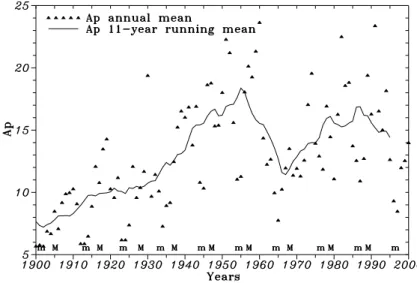
Fig. 5. Annual mean and 11-year
run-ning mean Ap index variations during the 20th century. Annual mean Ap in-dices prior to 1932 were reconstructed from aa indices available since 1868. Symbols (m) and (M) refer to years of solar cycle minimum and maximum.
and related variations in the thermospheric neutral composi-tion and temperature are the most probable mechanisms.
Although the proposed approach essentially deletes so-lar and geomagnetic activity effects and gives small and in-significant residual foF2 trend for the rising period of geo-magnetic activity (Table 4), most of these trends are negative. Slough (12:00 LT) also demonstrates negative and significant residual trend calculated over the 55-year period which in-clude both rising and falling periods in geomagnetic activity (Fig. 3, left-hand box).The same result was obtained on diur-nal variations for Slough (Table 6). Therefore, this result can hardly be coincidental. Negative foF2 trends may be consid-ered as a manifestation of the geomagnetic control which is not completely removed by the proposed method. Indeed, there is a very long-term increase in geomagnetic activity (e.g. Clilverd et al., 1998) which requires more smoother than Ap132 indices for its description. This long-term
in-crease takes place even for the analyzed period (Fig. 2, top), where a positive (K = 0.02 per year) trend is seen in the observed Ap132variation. Figure 2 (top) is only a fragment
of the general picture showing the increase in geomagnetic activity in the course of the 20th century (Fig. 5). This is a very delicate question which requires special consideration and is not discussed here.
An inclusion of a complementary linear δfoF2 trend to our analysis restores the unambiguity in the δfoF2132versus
Ap132 dependence (Figs. 3 and 4) and practically results in
a zero residual trend. Let us consider the sense of this com-plementary trend. The loop in the δfoF2132versus Ap132
de-pendence (Figs. 3 and 4), in principle, may be related to some changes in the Ap index determination after the middle of the 1960s (new stations, a modified method, etc.). The differ-ence between the two branches is not large (10–15%), but it is clearly seen in Figs. 3 and 4. On the other hand, Fig. 4 (top) shows that we have a new branch after 1990, shifted in the same direction and this can hardly be related to any changes in the method of the Ap index determination. Therefore, we should accept that observed δfoF2132values include an
addi-tional negative long-term trend which is not described by R12α and Ap132variations and the complementary trend just
com-pensates it. An intriguing explanation of the complementary trend could be related to the anthropogenic activity, such as, for instance, the increasing rate of rocket and satellite launch-ing, which leads to the thermosphere pollution (Kozlov and Smirnova, 1999; Adushkin et al., 2000). Indeed, switching on a complementary trend since 1960 (as the beginning of the cosmic era) improves to some extent the picture with the loops in Figs. 3 and 4, but the best results (the least SD) are obtained if the trend is switched on from the first year (1938) of the period analyzed (Table 7). It is impossible to link this result with the anthropogenic space pollution. Therefore, the only plausible explanation (as it is seen from now) of the complementary trend is a compensation of a negative trend initially presented in the observed δfoF2132values. This
neg-ative trend presumably has the same F2-layer storm nature as discussed by Mikhailov and Marin (2001) and is due to the earlier discussed very long-term increase in geomagnetic ac-tivity in the 20th century.
7 Conclusions
1. A new method to extract foF2 long-term trends, which are free to a great extent from solar and geomagnetic activity effects, has been proposed. This is achieved by using:
(a) a foF2 regression with Rα132 (where α is a fitting parameter) to remove the solar activity part from the foF2 long-term variations;
(b) relative rather than absolute δfoF2 deviations to find
δfoF2132(11-year running mean values);
(c) a regression with Ap132(11-year running mean Ap
values) to remove the geomagnetic activity effects from the foF2 long-term variations. Both δfoF2132
to provide the best correlation coefficients. Neither monthly nor annual mean δfoF2 values provide a high enough correlation with Ap indices and cannot be recommended for the foF2 trend analysis; (d) foF2 quiet time (Q-medians) rather than usual
monthly medians;
(e) all available δfoF2 observations rather than (m) or (m+M) year selections used in the previous version of our method;
(f) a −3 ± 1-year time shift between Ap132 and
δfoF2132 variations, to obtain the best correlation (the least SD). This time shift may be due to a large delay in the thermosphere reaction to the long-term changes in geomagnetic activity, with the physical mechanism of such an influence being unclear now.
2. The foF2 trends calculated for rising and falling phases of the long-term geomagnetic activity variation show neither latitudinal dependence nor any dependence on the phase being small and insignificant. The exis-tence of such dependencies for the trend magnitude was the basic point of the geomagnetic control concept by Mikhailov and Marin (2000, 2001).
3. The residual trend for Slough, calculated over the 55-year period, is small (Kr = −2.2 × 10⁻⁴ per year)
and significant. Such small foF2 trends have no prac-tical importance. On the other hand, negative (although primarily insignificant), residual trends that are calcu-lated over 10 ionosonde stations for a shorter period (31 years) may be considered as a manifestation of a very long-term geomagnetic activity increase, which did take place in the 20th century (Clilverd et al., 1998). But this effect cannot be removed even by using very smoothed indices, such as Ap132.
4. The main conclusion is that all revealed foF2 long-term variations (trends) may be attributed to the long-term solar and geomagnetic activity variations, i.e. they are of a natural origin. There is no indication of any manmade
foF2 trends.
Acknowledgement. This work was in part supported by the Russian
foundation for Fundamental Research under Grant 00–05–64189. Topical Editor M. Lester thanks M. Jarvis and P. Wilkinson for their help in evaluating this paper.
References
Adushkin, V. V., Kozlov, S. I., and Petrov A. V.: Ecological prob-lems and risks of the rocket and space technique impact on the environment, Moscow, Ankil, 638, 2000 (in Russian).
Bremer, J.: Ionospheric trends in mid-latitudes as a possible indica-tor of the atmospheric greenhouse effect, J. Atmos. Terr. Phys., 54, 1505–1511, 1992.
Bremer, J.: Trends in the ionospheric E- and F-regions over Europe, Ann. Geophysicae., 16, 986–996, 1998.
Clilverd, M. A., Clark, T. D. G., Clarke, E., and Rishbeth, H.: In-creased magnetic storm activity from 1868 to 1995, J. Atmos. Solar-Terr. Phys., 60, 1047–1056, 1998.
Danilov, A. D.: Long-term changes of the mesosphere and lower thermosphere temperature and composition, Adv. Space Res., 20, 2137–2147, 1997.
Danilov, A. D.: Review of long-term trends in the upper meso-sphere, thermosphere and ionomeso-sphere, Adv. Space Res., 22, 907– 915, 1998.
Danilov, A. D. and Mikhailov, A. V.: Spatial and seasonal variations of the foF2 long-term trends, Ann. Geophysicae., 17, 1239–1243, 1999.
Danilov, A. D. and Mikhailov, A. V.: F2-layer parameters long-term trends at the Argentine Islands and Port Stanley stations, Ann. Geophysicae, 19, 341–349, 2001.
Deminov, M. G., Garbatsevich, A. V., and Deminov R. G.: Climatic changes of the ionospheric F2-layer, Doklady RAN, 372, 383– 385, (in Russian), 2000.
Foppiano, A. J., Cid, L, and Jara, V.: Ionospheric long-term trends for South American mid-latitudes, J. Atmos. Solar-Terr. Phys., 61, 717–723, 1999.
Givishvili, G. V. and Leshchenko, L. N.: Possible proofs of pres-ence of technogenic impact on the midlatitude ionosphere, Dok-lady RAN, 334, 213–214, (in Russian), 1994.
Givishvili, G. V. and Leshchenko, L. N.: Dynamics of the cli-matic trends in the midlatitude ionospheric E-region, Geomag. i Aeronom., 35, 166–173, (in Russian), 1995.
Givishvili, G. V., Leshchenko, L. N., Shmeleva, O. P., and Ivanidze T. G.: Climatic trends of the mid-latitude upper atmosphere and ionosphere, J. Atmos. Terr. Phys., 57, 871–874, 1995.
Hedin, A. E.: MSIS-86 thermospheric model, J. Geophys. Res., 92, 4649–4662, 1987.
Jarvis, M. J., Jenkins, B., and Rodgers G. A.: Southern hemisphere observations of a long-term decrease in F-region altitude and thermospheric wind providing possible evidence for global ther-mospheric cooling, J. Geophys. Res., 103, 20 774–20 787, 1998. Ivanov-Kholodny, G. S.: Solar EU V quasi-biennial variations,
Phys. Chem. Earth (C), 25, 433–435, 2000.
Ivanov-Kholodny, G. S. and Chertoprud, V. Ye.: Analysis of ex-trema of quasi-biennial variations of solar activity, Astron. and Astrophys. Trans., 3, 81–85, 1992.
Kozlov, S. I. and Smirnova, N. V.: Estimation of the influence of helio-geophysical conditions on characteristics of ionospheric disturbances produced by rocket launches, Cosmic Res., 37, 507–514, (in Russian), 1999.
Marin, D., Mikhailov, A. V., de la Morena, B. A., and Herraiz, M.: Long-term hmF2 trends in the Eurasian longitudinal sector from the ground-based ionosonde observations, Ann. Geophysi-cae, 19, 761–772, 2001.
Mikhailov, A. V. and Marin, D.: Geomagnetic control of the foF2 long-term trends, Ann. Geophysicae, 18, 653–665, 2000. Mikhailov, A. V. and Marin, D.: An interpretation of the foF2 and
hmF2 long-term trends in the framework of the geomagnetic control concept, Ann. Geophysicae, 19, 733–748, 2001. Mikhailov, A. V. and Mikhailov, V. V.: Solar cycle variations of
annual mean noon foF2, Adv. Space Res., 15, 79–82, 1995. Mikhailov, A. V. and Mikhailov, V. V.: Indices for monthly median
foF2 and M(3000)F2 modeling and long-term prediction:
Iono-spheric index MF2, Inter. J. Geomag. and Aeronom., 1, 141–151, 1999.
Mikhailov, A. V., Skoblin, M. G, and F¨orster, M.: Daytime F2-layer positive storm effect at middle and lower latitudes, Ann. Geophysicae, 13, 532–540, 1995.
Muhtarov, P. and Kutiev, I.: Geomagnetically correlated statistical model (GCSM) for short-term prediction of ionospheric param-eters, Proc. of the 2nd COST 251 Workshop, 30–31 March 1998 Side, Turkey, 246–251, 1998.
Nusinov, A. A.: Dependence of intensity in lines of solar short-wave radiation on activity level, Geomag. i Aeronom., 24, 529–536, (in Russian), 1984.
Nusinov, A. A.: Models for prediction of EU V and X-ray solar ra-diation based on 10.7 cm radio emission, in: Proc. Workshop on Solar Electromagnetic Radiation for Solar Cycle 22, (Ed) Don-nely, R. F., Boulder, Co., July 1992, NOAA ERL. Boulder, Co., USA, 354–359, 1992.
Pollard, J. H.: A handbook of numerical and statistical techniques, Camb.Univ. Press, 1977.
Press, W. H., Teukolsky, S. A., Vetterling, W. T., and Flannery, P.: Numerical recipes in Fortran 77, Cambridge University Press, Cambridge, UK, 1992.
Rishbeth, H.: A greenhouse effect in the ionosphere?, Planet. Space Sci., 38, 945–948, 1990.
Rishbeth, H.: Long-term changes in the ionosphere, Adv. Space Res., 20, 2149–2155, 1997.
Rishbeth, H. and Barron, D. W.: Equilibrium electron distributions in the ionospheric F2-layer, J. Atmos. Terr. Phys., 18, 234–252, 1960.
Rishbeth, H. and Roble, R. G.: Cooling of the upper atmosphere by enhanced greenhouse gases − Modelling of thermospheric and ionospheric effects, Planet. Space Sci., 40, 1011–1026, 1992. Sharma, S. S., Chandra, H., and Vyas, G. D.: Long-term
iono-spheric trends over Ahmedabad, Geophys. Res. Lett., 26, 433– 436, 1999.
Ulich, T. and Turunen, E.: Evidence for long-term cooling of the upper atmosphere in ionospheric data, Geophys. Res. Lett., 24, 1103–1106, 1997.
Upadhyay, H. O. and Mahajan, K. K.: Atmospheric greenhouse ef-fect and ionospheric trends, Geophys. Res. Lett., 25, 3375–3378, 1998.
Zevakina, R. A. and Kiseleva, M. V.: F2-layer parameter varia-tions during positive disturbances related to phenomena in the magnetosphere and interplanetary medium, In: The diagnostics and modelling of the ionospheric disturbances, Nauka, Moscow, 151–167, (in Russian), 1978.