The Discovery of perceptual structure from visual co-occurrences in space and time

The Discovery of Perceptual Structure from Visual

Co-occurrences in Space and Time

by Phillip Isola

B.S., Computer Science, Yale University, 2008

Submitted to the Department of Brain and Cognitive Sciences in partial fulfillment of the requirements for the degree of

Doctor of Philosophy in Cognitive Science

at the Massachusetts Institute of Technology September 2015

@

2015 Massachusetts Institute of Technology All Rights Reserved.

Signature of Author:

Certified by:

Accepted by

Signature redacted

_

Department of Brain and Cognitive Sciences J Yn W1 2W015

Signature redacted

Edward H. Adelson John a Dorothy Wilson Professor of Vision Science Thesis Supervisor

SiQnature redacted

Matthew A. Wils61n Sherman Fairchild Professor of Neuroscience and Picower Scholar Director of Graduate Education for Brain and Cognitive Sciences

Al

-OF TEC8

JAN 2

6 2016

LIBRARIES_

ARCHIVES

u

,

:

The Discovery of Perceptual Structure from Visual Co-occurrences in

Space and Time

by Phillip Isola

Submitted to the Department of Brain and Cognitive Sciences in partial fulfillment of the requirements for the degree of

Doctor of Philosophy

Abstract

Although impressionists assure us that the world is just dabs of light, we cannot help but see surfaces and contours, objects and events. How can a visual system learn to organize pixels into these higher-level structures? In this thesis I argue that perceptual organization reflects statistical regularities in the environment. When visual primitives occur together much more often than one would expect by chance, we may learn to associate those primitives and to form a perceptual group.

The first half of the thesis deals with the identification of such groups at the pixel level. I show that low-level image statistics are surprisingly effective at higher-level segmentation. I present an algorithm that groups pixels by identifying meaningful co-occurrences in an image's color statistics. Consider a zebra. Black-next-to-white occurs suspiciously often, hinting that these colors have a common cause. I model these co-occurrences using pointwise mutual information (PMI). If the PMI between two colors is high, then the colors probably belong to the same object. Grouping pixels with high PMI reveals object segments. Separating pixels with low PMI marks perceived boundaries.

If simple color co-occurrences can tell us about object segments, what might more complex statistics tell us? The second half of the thesis investigates high dimensional visual data, such as image patches and video frames. In high dimensions, it is intractable to directly model co-occurrences. Instead, I show that modeling PMI can be posed as a simpler binary classification problem in which the goal is to predict if two primitives occur in the same spatial or temporal context. This allows us to model PMI associations between complex inputs. I demonstrate the effectiveness of this approach on three domains: discovering objects by associating image patches, discovering movie scenes by associating frames, and discovering place categories by associating geotagged photos.

Together, these results shed light on how a visual system can learn to organize raw sensory input into meaningful percepts.

Thesis Supervisor: Edward H. Adelson

Title: John and Dorothy Wilson Professor of Vision Science Thesis Committee: William T. Freeman, Joshua B. Tenenbaum

Acknowledgments

For me, the most enjoyable part of grad school has been getting to interact with so many creative and talented people. I've been fortunate to work with dozens of collaborators, friends, and mentors, and I'm grateful to them all. Here I will specify just a few who I worked especially closely with.

Thanks to Ted, my advisor, for his constant support and endless wisdom. I have very much appreciated the freedom he gave me to explore an eclectic array of projects. His disciplined approach and honest outlook on the limits of our knowledge has given me perspective on what it means to be a good scientist.

Thanks to Aude, for her mentorship throughout grad school, especially when I was just getting started. Her excitement is infectious, and her grand vision kept me inspired whenever day to day progress seemed slow.

Thanks to the other members of my committee, Bill and Josh. Thanks to Bill for showing me how an artistic creativity can be combined with rigorous engineering. Thanks to Josh for always providing deep and enjoyable conversation, and forcing me to think about the theoretical implication of my work.

Thanks to Antonio, who, along with Aude, fueled so much excitement and progress in my first few years working on memorability. Antonio's humor and creativity made working together always fun.

Thanks to Ce, who mentored me as an intern at Microsoft Research, for driving me not just to make things work, but also to understand why they work.

Thank you Daniel and Dilip, who were my co-authors on all the work described in this thesis. Daniel, thanks for always seeing the best side of each idea, for your excitement and ability to develop a half baked thought into a thorough experiment.

Dilip, thanks for your cool, collected, and kind approach to all things, and your skill at cutting away the fluff and getting at the main point.

Thank you to my all my collaborators on memorability. It has been gratifying to watch this research program develop beyond me. Thank you Devi for your clarity of thought, Wilma for your drive and ambition, and Aditya for your boundless ability to get cool things done. Thank you Zoya, not only for our work on memorability but also for sparking many fun projects beyond. Your ability to energize and organize people has been inspiring.

Thank you Joseph and Andrew, who have been constant friends as well as colleagues. I will miss our late night discussions at lab, even when they got a bit philosophical. Thank you Joseph for encouraging me to dream big. Thank you Andrew for keeping

me grounded, and always applying rigor and healthy skepticism to our work.

Thanks to all members of the two labs I have been part of, the T-Ruth group and the Oliva lab, and to the CSAIL vision group. It has been a pleasure working in such a welcoming and friendly environment.

Thanks to all my other friends during my time here, too numerous to name. Thanks for the conversations, the support, and the adventures.

Table of Contents

3 Abstract List of Figures List of Tables 1 Introduction

1.1 Perceptual organization and the role of structure in vision 1.2 Linking up visual data: similarity versus association . . . 1.3 An information-theoretic approach . . . . 1.4 Contributions . . . . 1.5 M y other work . . . .

2 Finding objects through suspicious coincidences in low-level vision 2.1 Introduction . . . . 2.2 Related work . . . . 2.3 Information-theoretic affinity . . . . 2.4 Learning the affinity function . . . . 2.5 Boundary detection . . . ... .. 2.6 Segmentation . . . .. 2.7 Experiments . . . .. ..... .. ... 17 19 . . . . 20 . . . . 22 . . . . 25 . . . . 26 . . . . 27 31 31 34 36 40 41 44 44 7 9

2.7.1 Is PMIP informative about object boundaries? . . . . 46

2.7.2 Benchmarks . . . . 47

2.7.3 Effect of p . . . . 53

2.8 D iscussion . . . . 55

3 Learning to group high-dimensional visual data 57 3.1 Related work . . . . 58

3.2 M odel . . . .. . .. . . . . 59

3.2.1 Modeling PMI explicitly with a GMM . . . . 63

3.2.2 Modeling PMI with a CNN . . . . 63

3.3 Learning visual associations . . . . 64

3.4 From associations to visual groups . . . . 69

3.4.1 Finding objects using patch associations . . . . 69

3.4.2 Segmenting movies using frame associations . . . . 71

3.4.3 Discovering place types using geospatial associations . . . . 72

3.5 D iscussion . . . . 73

4 Conclusion 75 4.1 Pixels versus patches . . . . 76

4.2 The effect of scale . . . . 77

4.3 Internal versus external statistics . . . . 78

4.4 Generative versus discriminative models of association . . . . 80

List of Figures

1.1 Illustration of perceptual organization. Statistical regularities in the world can be used to group raw pixels and patches into a variety of perceptual structures, such as object segments and contours. . . . . 20 1.2 Visual associations come in a wide variety of forms. Some associations are

perceived as visual similarity. Elsewhere two images may be associated but actually look quite dissimilar. The association may be semantic sameness, contextual proximity, a temporal link, stylistic similarity, or something else. Little work has modeled visual relationships beyond simple forms of similarity, such as the appearance similarity that relates the two photos of the Eiffel Tower above. While context models do exist, they usually operate over hand-designed semantic labels, rather than operating directly on raw images. This thesis looks for meaningful statistical associations in the raw data itself . . . . 24

2.1 From left to right: Input image; Contours recovered by the Sobel oper-ator [1051; Contours recovered by Dollar & Zitnick 2013 [28]; Contours recovered by Arbeliez et al. (gPb) [4]; Our recovered contours; Contours labeled by humans [4]. Sobel boundaries are crisp but poorly match hu-man drawn contours. More recent detectors are more accurate but blurry. Our method recovers boundaries that are both crisp and accurate. Our method does so by suppressing edges in highly textured regions such as the coral in the foreground. Here, white and gray pixels repeatedly occur next to each other. This pattern shows up as a suspicious coincidence in the image's statistics, and our method infers that these colors must therefore be part of the same object. Conversely, pixel pairs that strad-dle the coral/background edges are relatively rare and our model assigns

these pairs low affinity. . . . . 32 2.2 Our algorithm works by reasoning about the pointwise mutual

informa-tion (PMI) between neighboring image features. Middle column: Joint distribution of the luminance values of pairs of nearby pixels. Right col-umn: PMI between the luminance values of neighboring pixels in this zebra image. In the left image, the blue circle indicates a smooth region of the image where all points are on the same object. The green circle shows a region that contains an object boundary. The red circle shows a region with a strong luminance edge that nonetheless does not indicate an object boundary. Luminance pairs chosen from within each circle are plotted where they fall in the joint distribution and PMI functions. . . . 37

LIST OF FIGURES 11 2.3 A randomly scrambled version of the zebra image in Figure 2.2. The joint

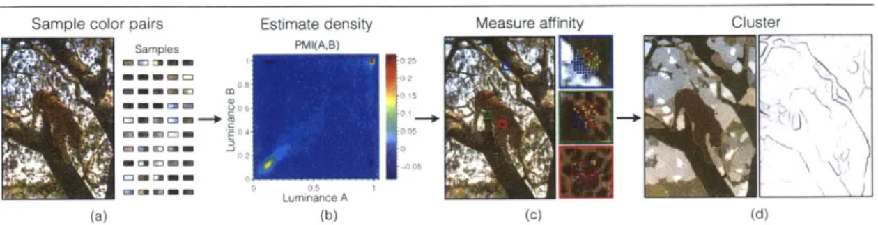
density for this image factors as P(A, B) ~ P(A)P(B). Non-symmetries in the distribution are due to finite samples; with infinite samples, the distribution would be perfectly separable. PMI is essentially comparing the hypothesis that the world looks like this scrambled image to the reality that the world looks like the zebra photo in Figure 2.2. . . . . 37 2.4 Boundary detection pipeline: (a) Sample color pairs within the image.

Red-blue dots represent pixel pair samples. (b) Estimate joint density P(A,B) and from this get PMI(A,B). (c) Measure affinity between each pair of pixels using PMI. Here we show the affinity between the center pixel in each patch and all neighboring pixels (hotter colors indicate greater affinity). Notice that there is low affinity across object boundaries but high affinity within textural regions. (d) Group pixels based on affinity (spectral clustering) to get segments and boundaries. . . . . 42 2.5 Here we show the probability that two nearby pixels are on the same

object segment as a function of various cues based on the pixel colors

A and B. From left to right the cues are: (a) color difference, (b) color

co-occurrence probability based on internal image statistics, (c) PMI based on external image statistics, (d) PMI based on internal image statistics, and (e) theoretical upper bound using the average labeling of

N -

1

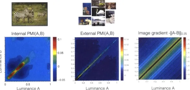
human labelers to predict the Nth. Color represents number of samples that make up each datapoint. Shaded error bars show three times standard error of the mean. Performance is quantified by treating each cue as a binary classifier (with variable threshold) and measuring AP and maximum F-measure for this classifier (sweeping over threshold). 44

2.6 The PMI function, over luminance values A and B, learned from internal image statistics (left) versus external statistics (middle). Internal statis-tics refers to measuring luminance co-occurrences in a particular image, in this case the zebra photo at the top left. External statistics refers to measuring luminance co-occurrences aggregated over the entire BSDS500 training set (example images from which are shown top middle). The in-ternal statistics suggest we should group black and white pixels, since these pairs show up with suspicious frequency on zebras. On most im-ages, however, we certainly should not group black and white pixels since usually dark and light things are separate objects. The external statis-tics convey this, assigning high affinity only to pixels with similar values (along the diagonal). External PMI therefore results in a function quite similar to the classical Sobel filter [105], which detects edges where the image gradient is high (rightmost plot). From this perspective, the Sobel filter measures statistical dissociations with respect to the statistics of average images, whereas our method detects edges with respect to the statistics of the specific test image we apply it to. . . . . 45 2.7 Precision-recall curve on BSDS500. Figure copied from [28] with our

results added. . . . . . . .. 47

2.8 Contour detection results for a few images in the BSDS500 test set, comparing our method to gPb [4] and SE [28]. In general, we suppress texture edges better (such as on the fish in the first row), and recover crisper contours (such as the leaves in upper-right of the fifth row). Note that here we show each method without edge-thinning (that is, we leave out non-maximal suppression in the case of SE, and we leave out OWT-UCM in the case of gPb and our method). . . . . 49

LIST OF FIGURES 13 2.9 Example segmentations for a few images in the BSDS500 test set,

com-paring the results of running OWT-UCM segmentation on our contours

and those of gPb [4]. . . . . 50 2.10 Color helps but many meaningful groupings can be found just in grayscale

im ages. . . . .

51

2.11 Here we show a zoomed in region of an image. Notice that our method

preserves the high frequency contour variation while gPb-owt-ucm does n ot. . . . .

52

2.12 Performance as a function of the maximum pixel distance allowed during

matching between detected boundaries and ground truth edges (referred to as r in the text). When r is large, boundaries can be loosely matched and all methods do well. When r is small, boundaries must be precisely localized, and this is where our method most outperforms the others. For our method in these plots, we use both color and variance features. 52 2.13 Left and middle: the effect of p (Equation 2.2) on performance at

pre-dicting whether or not two pixels are on the same object segment. Right: Boundary detection performance on BSDS500, comparing the parameter setting used in our benchmarks, p = 1.25, against using regular pointwise mutual information, i.e. p = I. . . . . 54 2.14 Three important properties of our approach: (a) it groups textures, (b)

it also groups non-repetitive but mutually diagnostic patterns, (c) and it can pick up on subtle shifts in color that are nonetheless statistically prom inent . . . . 55

3.1 We model the dependencies between two visual primitives - e.g., patches, frames, photos - occurring in the same spatial or temporal context. In each example above, the primitives are labeled A and B and the context is labeled by C. By learning which elements tend to appear near each other, we can discover visual groups such as objects (left), movie scenes (middle), and semantically related places (right). . . . . 58 3.2 Predictive qualities of different models for context and visual primitives.

We calculate the output of each model for a test set of unseen pairs of points. We then bin the outputs (x-axis values) and for each bin calculate the average value of the desired grouping principle Q (y-axis values, along with standard deviation). The context function for these plots is spatial adjacency and the grouping principle is segmentation (not used in training, obtained from Pascal VOC 2012). As can be seen (left), the joint distribution of visual primitives conditioned on context is non-informative about grouping. PMI, however, is highly informative about grouping (middle), as is the output of the discriminative model

P (CIA , B ) (right). . . . . 62

3.3 General structure of our CNNs for modeling functions of the form P(CIA, B). 65 3.4 Highly associated, but not trivially similar, patches discovered by the

model that learns patch associations. Each row shows pairs of highly associated patches. The patches in each pair are arranged one above the other. See text for details on how these patches are computed. . . . . . 66 3.5 Example object proposals. Out of 100 proposals per image, we show

those that best overlap the ground truth object masks. Average best overlap [60] and recall at a Jaccard index of 0.5 are superimposed over

LIST OF FIGURES 15 3.6 Object proposal results, evaluated on bounding boxes. Our unsupervised

method (labeled PMI) is competitive with state-of-the-art supervised algorithms at proposing up to around 100 objects. The far-right figure is for 50 proposals per image. ABO is the average best overlap metric from [60], J is Jaccard index. The papers corresponding to the the labels in the left plot are: BING [17], EdgeBoxes [124], LPO [61], Objectness [2],

GOP [60], Randomize Prim [74], Sel. Search [114]. . . . . 70 3.7 Movie scene segmentation results. On the left, we show a "movie

bar-code" for The Fellowship of the Ring; the top shows the DVD chapters and the bottom our recovered scene segmentation. On the right, we quantify our performance on this scene segmentation task; see text for details. . . . .

...71

3.8 Left: Clustering the LabelMe Outdoor dataset [66] into 8 groups us-ing PMI affinities. Random sample images are shown from each group. Right: Photo cluster purity versus number of clusters k. Note that PMI was learned on an independent dataset, the MIT City dataset [123]. . . 72 4.1 Boundary detection using pixel affinities (Chapter 2) versus patch

affini-ties (Chapter 3). Notice that the pixel affiniaffini-ties result in a finer-grained segmentation than the patch affinities. . . . . 76

List of Tables

2.1 Evaluation on BSDS500 . . . . 47 2.2 Evaluation on BSDS500 consensus edges [43]. We achieve a substantial

improvement over the state-of-the-art in the ODS and OIS measures. . . 53 3.1 Our method compared to baselines at predicting C (spatial or temporal

adjacency) and

Q

(semantic sameness) for three domains: image patch associations, video frame associations, and geospatial photo associations. In each column the first number is Average Precision and the second is F-measure at the threshold that maximizes this value. . . . . 65

Chapter 1

Introduction

Clown fish live next to sea anemones, lightning is always accompanied by thunder. When looking at the world around us, we constantly notice which things go with which.

These associations allow us to segment, interpret, and understand the world.

Why do we consider thunder and lightning to be associated? How did we learn the association in the first place? Through evolution and development, our hereditary line has been bombarded with a huge amount of raw visual data. Somewhere along the way we became able to make sense of it all. We began to see objects and events, rather than just of bunch of photons. How did we get from point A to point B? Put simply: how,

and why, do we group physical "stuff' into the perceptual "things"?

The focus of this thesis is on the unsupervised discovery of perceptual structure. I will describe how visual associations can be learned based on how often different colors, textures, and other patterns occur next to each other in our natural environment. Then I will show how to use these associations to uncover meaningful visual groups, including segments and contours, objects and movie scenes. Along the way, we will explore the utility of using statistical models that are highly specific to the subset of the world in which they will be applied. In addition, we will see how several problems in perceptual organization - including object segmentation, contour detection, and similarity measurements - can be posed as particular kinds of statistical association and dissociation.

What our eyes see What our mind sees

Object segments Figure-ground

Contours

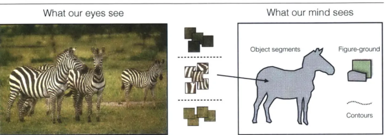
Figure 1.1: Illustration of perceptual organization. Statistical regularities in the world can be used to group raw pixels and patches into a variety of perceptual structures, such as object segments and contours.

This thesis deals with classical questions in perceptual science, about how and why we represent the world the way we do. A vast amount has been written on this. In order to situate us, I briefly review the prior work below.

M 1.1 Perceptual organization and the role of structure in vision

When we look at the world, we cannot help but see coherent structure. A bunch of birds forms a "flock", the black and white stripes of a zebra are grouped as a "texture", and, despite the idiom, we certainly can see the "forest" for the trees. Even if we look at unfamiliar visual worlds, like a Jackson Pollock painting or a fluffy cumulus cloud, we still see familiar shapes, symmetries, and groupings. This ability is known as perceptual organization: we organize the visual data around us into coherent percepts. The eyes take in a bunch of haphazard photons yet somewhere deep in the brain we arrange them into objects, contours, and layers (Figure 1.1). This thesis explores how we can replicate and explain some of these abilities with computational models.

An early attempt to systemize the rules of perceptual organization was given by the Gestalt psychologists. These scientists came up with a set of heuristic rules to explain how raw visual data gets bound up into coherent percepts. These rules deal mostly

Sec. 1.1. Perceptual organization and the role of structure in vision 21

with different notions of similarity and other heuristics, e.g., similarly colored circles are seen as a set, similarly oriented edge fragments are grouped into contours. This thesis adheres to an alternate and singular grouping principle: that perceptual groups are inferences about casual structure in the world. This idea also has a long history, going back at least to Helmholtz's notion of perception as unconscious inference [115],

and has since been developed by many researchers, e.g., [67, 90, 109, 120].

Rather than simply describing perceptual phenomenology, these researchers asked: what is perceptual organization for? Witkin and Tenenbaum proposed that the struc-tures we perceive can be viewed as explanations of the cause of the visual data [109, 120]. Certain visual patterns are highly unlikely to occur by accident, for example an arrange-ment of dots forming a perfect circle. We infer that someone, or some object, must have arranged the dots just so. The idea is that our visual system is on the lookout for non-accidental patterns because such patterns are clues toward the underlying physics and semantics of the world.

The idea of non-accidentalness has been widely applied in the vision literature. Among many other examples, non-accidentalness has been used to explain contour grouping [67], to disambiguate shape perception [40], and for image segmentation and clustering [35, 36].

This thesis presents a simple method for identifying non-accidental visual structure. Most previous works inferring non-accidental structures look for specific types of struc-ture, e.g., smooth contours [67] or specific 3D shapes [11]. In contrast, we look for a more general class of non-accidents: any visual events that occur together more often than you would expect by chance. An advantage of our approach is that we do not need to develop domain specific models for each new problem we consider. Chapter 3 demonstrates this property by using the same generic modeling steps for three rather different problems: object segmentation, movie scenes segmentation, and the discovery

of place types.

The idea of using co-occurrence rates to learn perceptual groups has some precedent. In an influential paper on auditory learning, Saffran et al. demonstrated that infants naturally pick up on regularities in the co-occurrence of sounds they hear, and they can use these to learn auditory groups

[94].

The authors suggested this might explain how infants learn to segment speech. Subsequent researchers showed that this kind of "statistical learning" also works in vision, with participants able to learn groupings of nonsense shapes based on their rates of co-occurence [39].

This approach to perceptual organization rests on modeling the pairwise statistics of visual primitives. Many previous works have used other pairwise visual relationships to uncover structure. I review those methods next.

* 1.2 Linking up visual data: similarity versus association

No pixel is an island. It is connected to the rest of the visual visual by a web of similarities, associations, and other relationships. Many approaches to identifying visual structure start by modeling the edges in this web.

Special focus has been devoted to appearance similarity. As far back as 1890, William James wrote that "a sense of sameness is the very keel and backbone of our thinking" [53]. Subsequent researchers have argued that similarity reveals how the brain organizes information, and underlies how we can generalize between alike stimuli (e.g., [98, 99, 111, 113]). Neuroscientists also use similarity to study cognitive organization. A currently popular technique is to measure "representational similarity": if two stimuli evoke similar patterns of brain activity, researchers infer that the brain represents those stimuli as alike [62]. This method can reveal visual object categories represented in inferotemporal cortex [20].

Sec. 1.2. Linking up visual data: similarity versus association 23

rules describe grouping based on some notion of similarity: similarity of appearance (law of similarity), of position (law of proximity), or of motion (law of common fate) [112].

In computer vision and machine learning, similarity is also a powerful organizing principle. Popular similarity-based methods include nearest-neighbor inference algo-rithms and kernel methods (see, e.g., [24] for a review), which model visual data as a matrix of pairwise similarity measurements. Most computational work on image sim-ilarity either hand-specifies a simsim-ilarity function (e.g., [119]) or learns simsim-ilarity from supervision (e.g., [72, 103, 108, 117]).

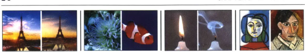
Nonetheless, the problem of visual similarity is far from solved. The majority of image similarity models in computer vision focus on "look-alikes" - i.e. images that have similar colors, textures, edges, and other perceptual features (see left-most panel of Figure 1.2). However, many pairs of images may be considered similar despite being very different at the pixel level (e.g., right-most panel of Figure 1.2). Other pairs will have many properties in common but nonetheless be considered dissimilar. Murphy & Medin give the example of a plum and lawnmower: both are less than 10,000 kg, both can be dropped, etc [82]. Psychological theories of similarity and categorization have long confronted this paradox: that two things can be wildly dissimilar in some ways yet

still be considered alike [41, 76, 79].

A key idea from this line of research is that for things to be considered alike, they need not be similar not in all aspects, but just must be similar in "ways that matter" (see [86] for further discussion). How can we identify which kinds of similarity matter and which do not?

While similarity may be a quite sensible grouping rule, this thesis proposes statistical association as a more fundamental principle. Statistical associations can be seen as a way of learning which kinds of similarity matter in a given domain. Indeed, I will show how certain kinds of visual similarity can be understood as approximate measures

Figure 1.2: Visual associations come in a wide variety of forms. Some associations are perceived as visual similarity. Elsewhere two images may be associated but actually look quite dissimilar. The association may be semantic sameness, contextual proximity, a temporal link, stylistic similarity, or something else. Little work has modeled visual relationships beyond simple forms of similarity, such as the appearance similarity that relates the two photos of the Eiffel Tower above. While context models do exist, they usually operate over hand-designed semantic labels, rather than operating directly on raw images. This thesis looks for meaningful statistical associations in the raw data itself.

of association (Chapter 2 Section 2.7.1 and Section 2.8, and throughout Chapter 3). This approach does away with the need to define what it means for two things to be similar and instead measures affinities purely as a function of objectively measurable information in the environment.

The central technical product of this thesis is an affinity measure, based on statistical association, that can be used as an alternative to similarity-based affinities. Such an affinity measure could be used to discover many kinds of visual structure, including low dimensional subspaces [92, 110] or graphs [57]. However, I will focus just on visual grouping. I follow a standard approach to using pairwise affinities for grouping [95]. First a graph is constructed in which visual primitives are the nodes and edge weights are given by the affinity between each pair of primitives. Then the graph is partitioned so that primitives with high affinity are assigned to the same partition and those with low affinity are assigned to separate partitions. There are several ways performance such a partitioning. Throughout this thesis, the particular method I use is spectral

Sec. 1.3. An information-theoretic approach 25

N 1.3 An information-theoretic approach

With this backdrop, we can now give a preview of the technical meat. How do we ac-tually measure visual associations? Our measure can be motivated as follows. Suppose you see two common events occur together, say a streetlight flickers right as a crow flies overhead. In all likelihood, you will discount this as mere coincidence. But when two rare events happen at once, perhaps hundreds of bats fill the midday sky as the sun enters an eclipse, we become suspicious that the events must be causally linked. Horace Barlow coined the term "suspicious coincidence" to describe events like this [8]. He defined these as cases in which the joint probability of two events is much higher than it would be if those events were independent (i.e., P(A, B)

>

P(A)P(B)). Such cases suggest that there is underlying structure that links the two events.

Barlow's idea is closely related to a measure of statistical association known as

pointwise mutual information (PMI) [37]:

PMI for two events A and B is defined as:

PMI(A, B) = log P(A (1.1)

P( A)P( B)'

Taking expectation over A and B results in the regular mutual information:

MI(A, B) = E[PMI(A, B)]. (1.2)

This quantity is the log of the ratio between the observed joint probability of {A, B} and the probability of this tuple were the two events independent. Equivalently, the ratio can be written as P(AIB) , that is, how much more likely is event A given that we

saw event B, compared to the base rate of event A.

What does PMI tell us about underlying causal structure? PMI will be zero if and only if A and B are independent events (as long as both A and B have non-zero

probability). Therefore, non-zero values of PMI indicate there is a dependency between the events. The sign of PMI also conveys information. Negative values indicate that observing A predicts that B will not occur. For example, if A and B are mutually exclusive, PMI will go to negative infinity. Negative values of PMI indicate dissociations, whereas positive values indicate associations. Two dissociated events are unlikely to be caused by the same underlying process. To group data, we therefore use the signed value of PMI as an affinity. This serves to group associated events and separates events that are either independent or dissociated.

Although not as prevalent as regular multual information, PMI does pop up here and there in the literature. In language modeling, it is commonly used to find collocations [15, 19]. Similar notions been have used to describe sparse coding in the brain [96] and to explain inferences of everyday cognition [42]. Closely related are methods that weigh the relevance or informativeness of some data based on how much more likely it is in a context of interest than in a background context. Such methods have been applied for information retrieval [106], mid-level visual learning [55, 104], and for visual clustering [35, 36].

M 1.4 Contributions

This thesis makes the following contributions. Our work:

1. Operationalizes classical ideas about non-accidentalness in perceptual organiza-tion.

2. Introduces a model of perceptual affinity based on statistical association rather than similarity.

3. Demonstrates the utility of local statistics for modeling these associations.

mid-Sec. 1.5. My other work 27

level grouping.

5. Derives an efficient way to scale up models of statistical association, simply using binary classifiers.

6. Provides general purposes machinery for applying the proposed framework to a variety of problems, by using deep convolutional neural nets.

* 1.5 My other work

During grad school I've had the opportunity to work on a wide variety of projects. A motivating question for me has been how do we represent knowledge about the world, and why do these representations exist? This thesis investigates representations in the form of visual groups - segments, objects, movie scenes, etc.

In parallel, I have been studying knowledge representation in the form of memories. What do we remember, and why do we remember it? In [48], [47], and [49], we found that people tend to remember photos of people, social scenes, and close up, interactive objects. Surprisingly, aesthetic photos were forgettable on average, and other high level assessments of quality, such as "interestingness", were also negatively correlated with memorability. This might be explained by the fact that most beautiful photos in our dataset were landscapes, and landscapes are devoid of memorable objects. Nonetheless, it became clear that memorability is measure distinct from other measures of visual im-pact, and, in contrast to measures like interestingness, memorability can be objectively quantified using behavioral experiments.

We extended our work to study the memorability of faces [6, 7], infographics [12], and words [68], and the topic has been produced a vibrant body of research from other students and groups as well, e.g., [58] and [73].

Of particular relevance to the topic of this thesis is our recent work modeling mem-orability from a statistical perspective. The general hypothesis is that the statistics of

our natural environment affect what we remember. This hypothesis is related to the classical idea in the literature that items that stand out from their context tend to be better remembered [59]. However, it has remained difficult to measure exactly what it means for a natural image to "stand out." In [13], we modeled this notion with a particular statistical model, measuring how unlikely it would be to see that image un-der the distribution images given by the surrounding context. This model can predict not only which images will be remembered, but also how a given image will change in memorability depending on the environment in which it is shown. It appears there, as it will in the rest of this thesis, that the statistics of the environment affect what knowledge our brains decide to represent.

I have also been interested in visual representations from an engineering perspec-tive. What are useful representations for 3D shapes, and for complex scenes? These questions lead to a line of work on collage-based representations. In [21] my co-authors and I introduced a representation for 3D shape that models the world as a collage of remembered surface fragments. In [46], I extended the approach to represent a full scene as a collage of remembered objects.

Most recently, I have been interested in representing data beyond a single image. What's an effective way to represent a whole collection of photos? In [51], my co-authors and I modeled a collection of photos of an object class, e.g., 'tomatoes', in terms of the states (e.g., 'unripe', 'ripe') depicted in that collection. We additionally looked at the transformations that link the states together (e.g., 'ripening'). The idea is that each image of a tomato is related to each other tomato image through a structured transformation. These transformations - 'ripening', 'aging', 'breaking' - describe highly specific kinds of visual relationships, imbued with rich semantics. The present thesis is also occupied with visual relationships, but of a much more basic class: co-occurrence rates of visual events in space and time.

Sec. 1.5. My other work 29

For a full list of my work during grad school please see my webpage at mit. edu/ phillipi.

Chapter 2

Finding objects through suspicious

coincidences in low-level vision

Partitioning images into semantically meaningful objects is an important component of many vision algorithms. In this chapter, we describe a method for detecting boundaries between objects based on a simple underlying principle: pixels belonging to the same object exhibit higher statistical dependencies than pixels belonging to different objects. We show how to derive an affinity measure based on this principle using pointwise mu-tual information, and we show that this measure is indeed a good predictor of whether or not two pixels reside on the same object. Using this affinity with spectral clustering, we can find object segments and boundaries in the image - achieving state-of-the-art results on the BSDS500 dataset. Our method produces pixel-level accurate boundaries while requiring minimal feature engineering.

This chapter is an extended version of [50].

* 2.1 Introduction

Semantically meaningful contour extraction has long been a central goal of computer vision. Such contours mark the boundary between physically separate objects and provide important cues for low- and high-level understanding of scene content. Ob-ject boundary cues have been used to aid in segmentation [4, 5, 63], obOb-ject detection

Sobel & Feldman Arbelez et al. Doller & Zitnick Our method Human labelers

1968 2011 (gPb) 2013 (SE)

Figure 2.1: From left to right: Input image; Contours recovered by the Sobel operator [105]; Contours recovered by Dollar & Zitnick 2013 [28]; Contours recovered by Ar-belAiez et al. (gPb)

[4];

Our recovered contours; Contours labeled by humans [4]. Sobel boundaries are crisp but poorly match human drawn contours. More recent detectors are more accurate but blurry. Our method recovers boundaries that are both crisp and accurate. Our method does so by suppressing edges in highly textured regions such as the coral in the foreground. Here, white and gray pixels repeatedly occur next to each other. This pattern shows up as a suspicious coincidence in the image's statistics,

and our method infers that these colors must therefore be part of the same object. Conversely, pixel pairs that straddle the coral/background edges are relatively rare and our model assigns these pairs low affinity.

and recognition [83, 102], and recovery of intrinsic scene properties such as shape, re-flectance, and illumination [9]. While there is no exact definition of the "objectness" of entities in a scene, datasets such as the BSDS500 segmentation dataset [4] provide a number of examples of human drawn contours, which serve as a good objective guide for the development of boundary detection algorithms. In light of the ill-posed nature of this problem, many different approaches to boundary detection have been developed

[4, 28, 65, 121].

As a motivation for our approach, first consider the photo on the left in Figure 2.1. In this image, the coral in the foreground exhibits a repeating pattern of white and gray stripes. We would like to group this entire pattern as part of a single object. One way to do so is to notice that white-next-to-gray co-occurs suspiciously often. If these colors were part of distinct objects, it would be quite unlikely to see them appear right next to each other so often. On the other hand, examine the blue coral in the background. Here, the coral's color is similar to the color of the water behind the coral. While the change in color is subtle along this border, it is in fact a rather unusual sort of change

Sec. 2.1. Introduction 33

- it only occurs on the narrow border where coral pixels abut background water pixels. Pixel pairs that straddle an object border tend to have a rare combination of colors.

These observations motivate the basic assumption underlying our method, which is that the statistical association between pixels within objects is high, whereas for pixels residing on different objects the statistical association is low. We will use this property to detect boundaries in natural images.

One of the challenges in accurate boundary detection is the seemingly inherent contradiction between the "correctness" of an edge (distinguishing between boundary and non-boundary edges) and "crispness" of the boundary (precisely localizing the boundary). The leading boundary detectors tend to use relatively large neighborhoods when building their features, even the most local ones. This results in edges which, correct as they may be, are inherently blurry. Because our method works on surprisingly simple features (namely pixel color values and very local variance information) we can achieve both accurate and crisp contours. Figure 2.1 shows this appealing properties of contours extracted using our method. The contours we get are highly detailed (as along the top of the coral in the foreground) and at the same time we are able to learn the local statistical regularities and suppress textural regions (such as the interior of the coral).

It may appear that there is a chicken and egg problem. To gather statistics within objects, we need to already have the object segmentation. This problem can be by-passed, however. We find that natural objects produce probability density functions (PDFs) that are well clustered. We can discover those clusters, and fit them by ker-nel density estimation, without explicitly identifying objects. This lets us distinguish common pixel pairs (arising within objects) from rare ones (arising at boundaries).

In this paper, we only look at highly localized features - pixel colors and color variance in 3x3 windows. It is clear, then, that we cannot derive long feature vectors

with sophisticated spatial and chromatic computations. How can we hope to get good performance? It turns out that there is much more information in the PDFs than one might at first imagine. By exploiting this information we can succeed.

Our main contribution is a simple, principled and unsupervised approach to contour detection. Our algorithm is competitive with other, heavily engineered methods. Unlike these previous methods, we use extremely local features, mostly at the pixel level, which allow us to find crisp and highly localized edges, thus outperforming other methods significantly when more exact edge localization is required. Finally, our method is unsupervised and is able to adapt to each given image independently. The resulting algorithm achieves state-of-the-art results on the BSDS500 segmentation dataset.

The rest of this chapter is organized as follows: we start by presenting related work, followed by a detailed description of our model. We then proceed to model validation, showing that the assumptions we make truly hold for natural images and ground truth contours. Then, we compare our method to current state-of-the-art boundary detection methods. Finally, we will discuss the implications of this work.

* 2.2 Related work

Contour/boundary detection and edge detection are classical problems in computer vision, and there is an immense literature on these topics. It is out of scope for this paper to give a full survey on the topic, so only a small relevant subset of works will be reviewed here.

The early approaches to contour detection relied on local measurements with linear filters. Classical examples are the Sobel [31], Roberts [89], Prewitt [85] and Canny [14] edge detectors, which all use local derivative filters of fixed scale and only a few orientations. Such detectors tend to overemphasize small, unimportant edges and lead to noisy contour maps which are hard to use for subsequent higher-level processing.

Sec. 2.2. Related work 35

The key challenge is to reduce gradients due to repeated or stochastic textures, without losing edges due to object boundaries.

As a result, over the years, larger (non-local) neighborhoods, multiple scales and orientations, and multiple feature types have been incorporated into contour detectors. In fact, all top-performing methods in recent years fall into this category. Martin et al. [78] define linear operators for a number of cues such as intensity, color and texture. The resulting features are fed into a regression classifier that predicts edge strength; this is the popular Pb metric which gives, for each pixel in the image the probability of a contour at that point. Dollar et al. [30] use supervised learning, along with a large number of features and multiple scales to learn edge prediction. The features are collected in local patches in the image.

Recently, Lim et al. [65] have used random forest based learning on image patches to achieve state-of-the-art results. Their key idea is to use a dictionary of human generated contours, called Sketch Tokens, as features for contours within a patch. The use of random forests makes inference fast. Doll6r and Zitnick [28] also use random forests, but they further combine it with structured prediction to provide real-time edge detection. Ren and Bo [87] use sparse coding and oriented gradients to learn dictionaries of contour patches. They achieve excellent contour detection results on BSDS500.

The above methods all use patch-level measurements to create contour maps, with non-overlapping patches making independent decisions. This often leads to noisy and broken contours which are less likely to be useful for further processing for object recognition or image segmentation. Global methods utilize local measurements and embed them into a a framework which minimizes a global cost over all disjoint pairs of patches. Early methods in this line of work include that of Shashua and Ullman [97]

programming approach to compute closed, smooth contours from local, disjoint edge fragments.

These globalization approaches tend to be fragile. More modern methods include a Conditional Random Field (CRF) presented in [88], which builds a probabilistic model for the completion problem, and uses loopy belief propagation to infer the closed con-tours. The highly successful gPb method of Arbel6ez et al. [4] embeds the local Pb measure into a spectral clustering framework [70, 101]. The resulting algorithm gives long, connected contours higher probability than short, disjoint contours.

The rarity of boundary patches has been studied in the literature before, e.g. [127]. We measure rarity based on pointwise mutual information [37] (PMI). PMI gives us a value per patch that allows us to build a pixel-level affinity matrix. This local affinity matrix is then embedded in a spectral clustering framework [4] to provide global contour information. PMI underlies many experiments in computational linguistics [15, 19] to learn word associations (pairs of words that are likely to occur together), and recently has been used for improving image categorization [10]. Other information-theoretic takes on segmentation have been previously explored, e.g., [81]. However, to the best of our knowledge, PMI has never been used for contour extraction or image segmentation.

* 2.3 Information-theoretic affinity

Consider the zebra in Figure 2.2. In this image, black stripes repeatedly occur next to white stripes. To a human eye, the stripes are grouped as a coherent object - the zebra. As discussed above, this intuitive grouping shows up in the image statistics: black and white pixels commonly co-occur next to one another, while white-green combinations are rarer, suggesting a possible object boundary where a white stripe meets the green background.

Sec. 2.3. Information-theoretic affinity 37 loq P(AB) 0.8 o 0.6 E 0.4 0. 0.2 0 0.5 Luminance A _ PMI(A,B)

Ia

-4.8 -475 4.7 -4.65 0

I

I

0.5 Luminance A -0.1 0.05 -0 --0 05

Figure 2.2: Our algorithm works by reasoning about the pointwise mutual information (PMI) between neighboring image features. Middle column: Joint distribution of the luminance values of pairs of nearby pixels. Right column: PMI between the luminance values of neighboring pixels in this zebra image. In the left image, the blue circle indicates a smooth region of the image where all points are on the same object. The green circle shows a region that contains an object boundary. The red circle shows a region with a strong luminance edge that nonetheless does not indicate an object boundary. Luminance pairs chosen from within each circle are plotted where they fall in the joint distribution and PMI functions.

log P(A,B) C cc C E :3 Luminance A

Figure 2.3: A randomly scrambled version of the zebra image in Figure 2.2. The joint density for this image factors as P(A, B) ~ P(A)P(B). Non-symmetries in the distribution are due to finite samples; with infinite samples, the distribution would be perfectly separable. PMI is essentially comparing the hypothesis that the world looks like this scrambled image to the reality that the world looks like the zebra photo in Figure 2.2.

image features, based on statistical association. We denote a generic pair of neighbor-ing features by random variables A and B, and investigate the joint distribution over pairings {A, B}.

37 Sec. 2.3. Information-theoretic affinity

Let p(A, B; d) be the joint probability of features A and B occurring at a Euclidean distance of d pixels apart. We define P(A, B) by computing probabilities over multiple distances:

P(A, B) = : w(d)p(A, B; d), (2.1)

d=do

where w is a weighting function which decays monotonically with distance d (Gaussian in our implementation), and Z is a normalization constant. We take the marginals of this distribution to get P(A) and P(B).

In order to pick out object boundaries, a first guess might be that affinity should be measured with joint probability P(A, B). After all, features that always occur together probably should be grouped together. For the zebra image in Figure 2.2, the joint distribution over luminance values of nearby pixels is shown in the middle column. Overlaid on the zebra image are three sets of pixel pairs in the colored circles. These pairs correspond to pairs

{A,

B} in our model. The pair of pixels in the blue circle are

both on the same object and the joint probability of their colors - green next to green

-is high. The pair in the bright green circle straddles an object boundary and the joint probability of the colors of this pair - black next to green - is correspondingly low.

Now consider the pair in the red circle. There is no physical object boundary on the edge of this zebra stripe. However, the joint probability is actually lower for this pair than for the pair in the green circle, where an object boundary did in fact exist. This demonstrates a shortcoming of using joint probability as a measure of affinity. Because there are simply more green pixels in the image than white pixels, there are more chances for green accidentally show up next to any arbitrary other color - that is, the joint probability of green with any other color is inflated by the fact that most pixels in the image are green.

Sec. 2.3. Information-theoretic affinity 39

affinity with a statistic related to pointwise mutual information:

P(A, B)P

PMI (A, B) = log ' . (2.2)

P(A)P(B)

When p = 1, PMI is precisely the pointwise mutual information between A and B discussed in the introduction of this thesis. To recap, this quantity is the log of the ratio between the observed joint probability of {A, B} in the image and the probability of this tuple were the two features independent. Equivalently, the ratio can be written as P(A) , that is, how much more likely is observing A given that we saw B in the same local region, compared to the base rate of observing A in the image. When p = 2, we have a stronger condition: in that case the ratio in the log becomes P(AIB)P(BIA). That is, observing A should imply that B will be nearby and vice versa. As it is unclear a priori which setting of p would lead to the best segmentation results, we instead treat

p as a free parameter and select its value to optimize performance on a training set of

images (see Section 2.4).

In the right column of Figure 2.2, we see the pointwise mutual information over features A and B. This metric appropriately corrects for the baseline rarities of white and black pixels versus gray and green pixels. As a result, the pixel pair between the stripes (red circle), is rated as more strongly mutually informative than the pixel pair that straddles the boundary (green circle). In Section 2.7.1 we empirically validate that PMI is indeed predictive of whether or not two points are on the same object.

Figure 2.3 shows what the zebra image would look like if adjacent colors were ac-tually independent. The log joint distribution over this scrambled image is plotted to the right, which is approximately equal to log P(A)P(B). PMI is essentially measuring how far away the statistics of the actual zebra image are from this unstructured version of the zebra image. Specifically, the PMI function for the zebra image (right column of Figure 2.2) is equal to the distribution in the middle column of Figure 2.2 minus the

distribution on the right of Figure 2.3 (up to sampling approximations).

* 2.4 Learning the affinity function

In this section we describe how we model P(A, B), from which we can derive PMIp(A, B). The pipeline for this learning is depicted in Figure 2.4(a) and (b). For each image on which we wish to measure affinities, we learn P(A, B) specific to that image itself. Extensions of our approach could learn P(A, B) from any type of dataset: videos, photo collections, images of a specific object class, etc. However, we find that modeling

P(A, B) with respect to the internal statistics of each test image is an effective approach

for unsupervised boundary detection. The utility of internal image statistics has been previously demonstrated in the context of super-resolution and denoising [125] as well as saliency prediction [75].

Because natural images are piecewise smooth, the empirical distribution P(A, B) for most images will be dominated by the diagonal A ~ B (as in Figure 2.2). However, we are interested in the low probability, off-diagonal regions of the PDF. These off diagonal regions are where we find changes, including both repetitive, textural changes

and object boundaries. In order to suppress texture while still detecting subtle object boundaries, we need a model that is able to capture the low probability regions of

P(A, B).

We use a nonparametric kernel density estimator [84] since it has high capacity without requiring an increase in feature dimensionality. We also experimented with a Gaussian Mixture Model but were unable to achieve the same performance as kernel density estimators.

Kernel density estimation places a kernel of probability density around every sample point. We need to specify on the form of the kernel and the number of samples. We used Epanechnikov kernels (i.e. truncated quadratics) owing to their computational

Sec. 2.5. Boundary detection

41

efficiency and their optimality properties [33], and we place kernels at 10000 sample points per image. Samples are drawn uniformly at random from all locations in the image. First a random position x in the image is sampled. Then features A and B are sampled from image locations around x, such that A and B are d pixels apart. The sampling is done with weighting function w(d), which is monotonically decreasing and gives maximum weight to d = 2. The vast majority of samples pairs {A, B} are within distance d = 4 pixels of each other.

Epanechnikov kernels have one free parameter per feature dimension: the bandwidth of the kernel in that dimension. We select the bandwidth for each dimension through leave-one-out cross-validation to maximize the data likelihood. Specifically, we compute the likelihood of each sample given a kernel density model built from all the remaining samples. As a further detail, we bound the bandwidth to fall in the range [0.01, 0.1] (with features scaled between [0,1]) - this helps prevent overfitting to imperceptible details in the image, such as jpeg artifacts in a blank sky. To speed up evaluation of the kernel density model, we use the kd-tree implementation of Ihler and Mandel [44]. In addition, we smooth our calculation of PMI slightly by adding a small regularization constant to the numerator and denominator of Eq. 2.2.

Our model has one other free parameter, p. We choose p by selecting the value that gives the best performance on a training set of images completely independent of the test set, finding p = 1.25 to perform best.

* 2.5 Boundary detection

Armed with an affinity function to tell us how pixels should be grouped in an image, the next step is to use this affinity function for boundary detection (Figure 2.4 (c) and (d)). Spectral clustering methods are ideally suited in our present case since they operate on affinity functions.

Sample color pairs Estimate density Measure affinity Cluster

Samples PMI(A,B)

(a) (b) (c) (d)

Figure 2.4: Boundary detection pipeline: (a) Sample color pairs within the image. Red-blue dots represent pixel pair samples. (b) Estimate

joint

density P(A,B) and from this get PMI(AB). (c) Measure affinity between each pair of pixels using PMI. Here we show the affinity between the center pixel in each patch and all neighboring pixels (hotter colors indicate greater affinity). Notice that there is low affinity across object boundaries but high affinity within textural regions. (d) Group pixels based on affinity (spectral clustering) to get segments and boundaries.

Spectral

clustering

was introduced in the context of image segmentation as a way to approximately solve the Normalized Cuts objective

[1001.

Normalized Cuts segments an image so as to maximize within segment affinity and minimize between segment affinity. To detect boundaries, we apply a spectral clustering using our affinity function, following the current state-of-the-art solution to this problem, gPb

[41.

As input to spectral clustering, we require an affinity matrix, W. We get this from our affinity function PMI, as follows. Let i and j be indices into image pixels. At each

pixel, we define a feature vector f. Then, we define:

Wu= eP~~ay (2.3)

The exponentiated values give us better performance than the raw PMI, values. Since our model for feature pairings was

learned

on nearby pixels, we only evaluate the affinity matrix for pixels within a radius of 5 pixels from one another. Remaining affinities are set to

0.