HAL Id: insu-01681392
https://hal-insu.archives-ouvertes.fr/insu-01681392
Submitted on 17 Nov 2020
HAL is a multi-disciplinary open access
archive for the deposit and dissemination of
sci-entific research documents, whether they are
pub-lished or not. The documents may come from
teaching and research institutions in France or
abroad, or from public or private research centers.
L’archive ouverte pluridisciplinaire HAL, est
destinée au dépôt et à la diffusion de documents
scientifiques de niveau recherche, publiés ou non,
émanant des établissements d’enseignement et de
recherche français ou étrangers, des laboratoires
publics ou privés.
Investigations of the Mars Upper Atmosphere with
ExoMars Trace Gas Orbiter
Miguel Lopez-Valverde, Jean-Claude Gérard, Francisco González-Galindo,
Ann-Carine Vandaele, Ian Thomas, Oleg Korablev, Nikolai Ignatiev, Anna
Fedorova, Franck Montmessin, Anni Määttänen, et al.
To cite this version:
Miguel Lopez-Valverde, Jean-Claude Gérard, Francisco González-Galindo, Ann-Carine Vandaele, Ian
Thomas, et al.. Investigations of the Mars Upper Atmosphere with ExoMars Trace Gas Orbiter.
Space Science Reviews, Springer Verlag, 2018, 214 (1), pp.artcle 29. �10.1007/s11214-017-0463-4�.
�insu-01681392�
Investigations of the Mars upper atmosphere with
Exomars Trace Gas Orbiter
Miguel A. L´opez-Valverde1
· Jean-Claude Gerard2
· Francisco Gonz´alez-Galindo1 · Ann-Carine Vandaele3 · Ian Thomas3 · Oleg Korablev4 · Nikolai Ignatiev4 · Anna Fedorova 4 · Franck Montmessin5 · Anni M¨a¨att¨anen5 · Sabrina Guilbon5 · Franck Lefevre6
· Manish R. Patel7 · Sergio Jim´enez-Monferrer1 · Maya Garc´ıa-Comas1 · Alejandro Cardesin8 · Colin F. Wilson9 · R. T. Clancy10 · Armin Kleinb¨ohl11 · Daniel J. McCleese11 · David M. Kass11
· Nick M. Schneider12 · Michael S. Chaffin12 · Jos´e Juan L´opez-Moreno1 · Julio Rodr´ıguez1
Received: date / Accepted: date
M. A. L´opez-Valverde
Instituto de Astrof`ısica de Andaluc´ıa/CSIC, Granada, Spain Tel.: +34-958-121311 , Fax: +34-958-814530 , E-mail: valverde@iaa.es J.-C. Gerard
Laboratoire de Physique Atmosphrique et Plantaire, Universit de Li`ege, Belgium
F. Gonz´alez-Galindo, S. Jim´enez-Monferrer and M. Garc`ıa-Comas and J. J. L´opez-Moreno and J. Rodr´ıguez
IAA/CSIC, Granada, Spain A.-C. Vandaele and I. Thomas IASB, Brussels, Belgium
O. Korablev and N. Ignatiev and A. Fedorova IKI, Moscow, Russia
F. Montmessin and A. M¨a¨att¨anen and S. Guilbon
LATMOS/IPSL, UVSQ Universit´e Paris-Saclay, UPMC Univ. Paris 06, CNRS, Guyancourt, France
F. Lefevre
LATMOS/IPSL, UPMC Univ. Paris 06 Sorbonne Universit´es, UVSQ, CNRS, Paris, France M. R. Patel
Open University, Milton-Keynes, UK A. Cardesin
ESAC, Madrid, Spain C. F. Wilson
Physics Department, Oxford University, UK R. Tood Clancy
Abstract The Martian mesosphere and thermosphere, the region above about 60 km, is not the primary target of the Exomars 2016 mission but its Trace Gas Orbiter (TGO) can explore it and address many interesting issues, either in-situ during the aerobraking period or remotely during the regular mission. In the aer-obraking phase TGO peeks into thermospheric densities and temperatures, in a broad range of latitudes and during a long continuous period. TGO carries two instruments designed for the detection of trace species, NOMAD and ACS, which will use the solar occultation technique. Their regular sounding at the terminator up to very high altitudes in many different molecular bands will represents the first time that an extensive and precise dataset of densities and hopefully tem-peratures are obtained at those altitudes and local times on Mars. But there are additional capabilities in TGO for studying the upper atmosphere of Mars, and we review them briefly. Our simulations suggest that airglow emissions from the UV to the IR might be observed outside the terminator. If eventually confirmed from orbit, they would supply new information about atmospheric dynamics and variability. However, their optimal exploitation requires a special spacecraft point-ing, currently not considered in the regular operations but feasible in our opinion. We discuss the synergy between the TGO instruments, specially the wide spectral range achieved by combining them. We also encourage coordinated operations with other Mars-observing missions capable of supplying simultaneous measurements of its upper atmosphere.
Keywords Mars · Exomars · NOMAD · ACS · Upper Atmosphere · aerobraking · airglow · remote sounding
1 Introduction
Exomars 2016 was launched on March 14th, 2016, carrying two major modules: (i) the Trace Gas Orbiter, or TGO in short, a spacecraft in orbit around Mars with four remote sounding instruments on board, and (ii) the Schiaparelli surface platform. The release of the Schiaparelli module and the successful insertion of TGO into Mars orbit took place on October 19th, 2016 ([31]). A special period of high elliptic 4-sols (sol = Martian day) orbits around Mars immediately started, the so called Mars Capture Orbit phase (MCO hereinafter), which lasted for about two months. Around mid January 2017 maneuvers to change the orbit inclination and to lower the apocentre took place, shifting the orbital plane of TGO from the original nearly equatorial to a nearly polar orientation and reducing the period to about 1 day. In March 2017, a phase of aerobraking started, which will last for months, possibly until February 2018, when the regular operations should start. The final orbit will have a 74o
inclination and a period of 2 h. The driving scientific goals of TGO and the individual instruments on-board can be found in several accompanying papers (Vandaele et al, 2017 [131]; Korablev et al., 2017 [72]).
The Martian mesosphere (altitudes between about 60 km and 120 km) and thermosphere (above about 120 km) are not the primary targets of the Exomars
A. Kleinb¨ohl and D. J. McCleese and D. M. Kass JPL, Caltech, Pasadena, CA, USA
N. M. Schneider and M. S. Chaffin LASP, Boulder, CO, USA
high in the Mars atmosphere, and the orbit configuration offers possibilities to ad-dress a number of open problems at high altitudes. Here we review these possibili-ties and their scientific interest, and try to motivate the Mars research community to pay attention to the upcoming data from the mission for exploiting them and to think about further upper atmosphere studies.
A short review of open problems in our understanding of the Mars upper at-mosphere is discussed in Sect. 2 below.This is a selection which does not aim to
be exhaustive. This work benefits from and builds upon a few recent and more
extensive reviews written in preparation for the MAVEN mission (Bougher et al., 2014 [10]). We expect the Exomars 2016 TGO shall also contribute to some of the MAVEN goals and, further, to complement them in an altitude region not properly covered by MAVEN. In Sect. 3 we describe the nominal operations of TGO and a few simulations to illustrate the science that can be obtained from orbit with the key instruments. In Sect. 4 we discuss additional studies of the upper atmosphere that could be tackled with TGO, outside its standard opera-tion modes. We will also propose observaopera-tions to exploit the TGO instruments synergy, the aerobraking phase of the mission, as well as correlation campaigns with other instrumentation and projects, from the European Mars Express and the NASA missions Mars Reconnaissance Orbiter (MRO) and MAVEN, to the future James Webb Space Telescope (JWST in short). The major conclusions and recommendations are summarized in Sect. 5.
2 Brief review of Mars upper atmosphere’s open questions
As reviewed by Leblanc et al, 2006 [74] (see references therein), five methods have been used so far to probe the Martian upper atmosphere, in-situ mea-surements, aerobraking and orbital decay, radio-occultation and remote sound-ing. In situ observations have been performed by descent probes like Viking and Pathfinder/ASIMET or the latest Schiaparelli/Exomars 2016. Accelerometer mea-surements of total density versus altitude have been performed during the aero-braking phase of several Mars orbiters, exploring atmospheric heights ranging from 110 to 180 km (Zurek et al., 2015 [147], Zurek et al., 2017 [146], Bougher et al., 2017 [9]). Radio occultation methods have provided the electron density profiles above 75 km, and remote sensing of airglow emissions of the upper atmosphere have been used since the early Mars missions (Bougher et al., 2017 [9] and references therein). Additionally, theoretical efforts have also focused in the development of numerical models of the upper atmosphere, tackling radiative (Wolff et al., 2017 [141], and references therein) and dynamical problems of the upper atmosphere (Bougher et al., 2014 [10] and references therein). Notably, the extension in altitude of the general circulation models now permits the global analysis from the surface to the exosphere, including links with the lower atmosphere (Bougher et al., 2006 [8], Spiga et al., 2012 [121], Gonz´alez-Galindo et al., 2015 [53], Bougher et al., 2015 [11]). The plethora of studies revealed, first of all, the need for more measurements and an example intended to fill in that need is the MAVEN mission (Jakosky et al., 2015 [63]). This mission is supplying a significant amount of new in-situ and remotely sensed measurements with its suite of instruments. This includes a mass spectrometer (NGIMS) for neutral and ion densities, a Langmuir probe (LPW)
for electron densities and temperatures, and an UV spectrograph (IUVS) yielding selected neutral and ion densities from dayglow emissions and stellar occultations. Here we paint a succinct panorama of half a dozen open and interesting issues in our understanding of the Mars upper atmosphere, which clearly demand fur-ther attention and which the TGO data may permit insightful analysis, both as a standalone experiment and as a new tool in combination with previous and future data.
I EUV and non-EUV heating sources The atmospheric heating by the solar flux in the extreme UV is the dominant heating source of the Martian thermo-sphere and the major driver of the daily variations. Still it is poorly described nowadays, with an essentially altituindependent percentage of energy de-position based on theoretical studies in the 70s which require revision (Fox and Dalgarno, 1979 [40]). Such revision ideally should be based on new ob-servations in a range of altitudes starting and above the mesopause (about 120-125 km on Mars). In the lower thermosphere in particular (120-160 km), where the strongest temperature gradient occurs, the atmospheric energy bud-get is complemented by diverse factors whose competing roles are not fully understood. These include radiation (emissions and solar absorptions in the IR and near-IR under non-local thermodynamic equilibrium), the global dy-namics (inter-hemispheric transport of species and downwelling and diabatic heating in polar regions), and the small scale perturbations (waves and tides propagating up to thermospheric altitudes). TGO density and temperature determinations are expected in the whole mesosphere and lower thermosphere (MLT in short, 60-160 km), which should bring new data and impetus to this issue.
II Day/Night Changes
Daily changes in the atmospheric basic structure (density and temperature) and composition are specially strong at the terminator (the day-night transi-tion), and at high altitudes. They are part of the atmospheric natural variabil-ity and affect its structure at all altitudes above. Their precise understanding is important for reliable predictions for the aerobraking of orbiting satellites. Several open issues are closely related to local time variations; one example is the occurrence of CO2 mesospheric clouds (Gonz´alez-Galindo et al., 2011
[54]). According to models, one of the two periods when the clouds are fa-vored is during the first part of the Martian year around sunrise and sunset, when they are confined near the equator, where the thermal tides have largest amplitudes and produce temperature minima sufficiently close to the cold con-densation values. As shown in Figure 1, the altitudes of temperature minima vary by 30 km between the two terminators due to the thermal tides. Day-night ocurrences in clouds show a trend in agreement with the models, but the precise quantitative prediction at the terminator has not been confirmed by mesospheric cloud measurements given the incomplete local time coverage of previous satellite observations. Mesospheric clouds have also been observed in the daylight hemisphere by IUVS/MAVEN thanks to solar scattering in the UV (Deighan et al., 2017 [27]). The terminator will be described with unprecedented detail by TGO systematic observations from the ground up to the thermosphere. These TGO observations will nicely complement MAVEN measurements outside the terminator.
Fig. 1 Difference between the atmospheric temperature and the condensation temperature of CO2, as a function of altitude and local time, for (Ls=120 150, Lon=0, Lat=0), as simulated
by the LMD-MarsGCM. After (Gonz´alez-Galindo et al., 2011 [54]).
III Homopause/Mesopause variability
The location and temporal variation of these two layers are considered as prime indicators of our understanding of the upper atmosphere of the terres-trial planets, and certainly this is the case of Mars, now and during its long term evolution (Ehlmann et al., 2017 [29]). They depend on many dynamical and radiative processes, not only locally at their precise altitudes, or on the lower atmosphere below (Jakosky et al., 2017 [64]), but also on a global scale (Gonz´alez-Galindo et al., 2009 [52]). Further, they are key to understand pro-cesses like photochemical escape and the current atmosphere’s energy budget. The tracking of their variability requires systematic observations in the range of altitudes around 100-130 km on Mars (or an even wider range, according to Jakosky et al., 2017 [64]). This is possibly the coldest and most difficult region to sound, both from remote observations using emission spectroscopy and from in-situ satellite periapsis, normally at higher altitudes. Solar occul-tation observations present possibly the best tool to sound this atmospheric region. The deep-dips campaigns of MAVEN down to 120 km and the system-atic mapping with TGO of the mesopause and homopause should complement and supply unique information to describe these critical layers.
IV Wave coupling with lower atmosphere
The coupling of the lower and upper atmosphere occurs via propagation of waves, diffusion of species, the general circulation and local thermal expan-sion due to dust storms (Bougher et al., 2014 [10]). Gravity waves, tides and planetary waves at thermospheric altitudes were examined during the
aer-obraking of the MGS and MO spacecrafts (Forbes et al., 2002 [37]; Fritts et al., 2006 [41]) and more recently with MAVEN (Yigit et al., 2015 [145], Zurek et al., 2017 [146]). Density variations recently found as high as the exobase by MAVEN have been attributed to gravity waves (Yigit et al., 2015 [145]; Terada et al., 2017 [128]). Efforts have been also devoted recently to the parameterization of sub-grid scale gravity waves into GCMs (Yigit et al., 2008; Medvedev et al., 2015) and simulation of gravity wave propagation with mesoscale models (Spiga et al., 2012). Gravity waves may play an important role in the deposition of energy in the MLT region in Mars although their role on the global dynamics seems to be less important than it is on Earth (Bougher et. al, 2006 [8]). Recent modeling of convectively driven gravity waves suggests that the propagation of short-period modes produced by vig-orous convection can be so fast in the Martian atmosphere that such waves could reach even the upper thermosphere (Imamura et al., 2016 [61]). The propagation of gravity waves continues posing a challenge to models for two reasons. One is the intrinsic difficulty in the description of sources and prop-agation, both within 3-D global models and with 1-D constrained models. An example is the discussion over which, topography or convection, dominate the generation of these waves (Imamura et al., 2016 [61]). The other is the lack of measurements suited for their detection: in particular 2-D instantaneous mapping in the vertical and the horizontal, like that performed on Venus by VIRTIS/Venus Express; Gilli et al, 2009 [49], or like tomographic observa-tions of the Earth’s upper atmosphere (Song et al., 2017 [118]). The TGO long aerobraking phase and the systematic observations during solar occulta-tion can be very valuable for this purpose. Furthermore, measurements during non-nominal operation modes, as those proposed in section 4.2, could also be very informative to describe further the small-period gravity waves.
V Photochemistry and escape of water vapor
As discussed by Bougher et al. 2014 [10]) regular observations of the neu-tral species are needed to understand escape processes, in addition to their variability with local times, latitudes and seasons, and the solar cycle. This is the case of the light species which form the Martian corona, or exosphere, and their escape rates. One of the all important species is H and the D/H ratio, linked to the escape of water vapor, which in the classical photochem-ical frame, takes place first by diffusion of H2 upwards to the homopause layer, and then throughout the thermosphere, preferentially in the atomic form (Clarke et al., 2014 [22]). Recent measurements of H and D abundances by IUVS/MAVEN in the far-UV (Chaffin et al., 2014 [14]; Clarke et al., 2017 [23]) show large variations of both H and D Lyman alpha emissions, with excursions up to very high D/H ratios at thermospheric altitudes over the course of a Martian year, well above the value ∼ 5 found at low altitudes. The variations contain a clear seasonal component which is not entirely ex-plained in terms of EUV solar radiation (Chaufray et al, 2015 [15]). Tenta-tive explanations propose elevated H2O abundance at mesospheric altitudes,
perhaps linked to a convectively active lower atmosphere (Fedorova et al., 2015 [33]). The critical mesospheric and lower thermospheric altitudes will be systematically sounded by TGO, and further, it is expected to measure D/H ratios and H2O abundance profiles with unprecedented precision. These
NGIMS on MAVEN, should be crucial for our understanding of the escape of water, including the challenging lower-to-upper atmosphere diffusion and its implications for the long term escape and evolution of species like water on Mars.
VI Airglow and non-thermal emissions
Airglow emissions in the UV and visible, together with IR emissions under non-local thermodynamic equilibrium situations, are distinct features of the upper atmospheres of the terrestrial planets. They strongly depend on key geophysical parameters, like temperature and species abundances and atmo-spheric chemistry (and therefore escape), but also on solar inputs (radiant fluxes and particle precipitation), photochemical reactions and ionization, and molecular energy transfer processes. The upper atmospheres are natural labo-ratories where much can be learned about all these parameters and processes, and viceversa, their emission rates are key ingredients in the radiative balance at high altitudes (Barth et al., 1992 [3], Strobel, 2002 [127], Lopez-Puertas and Taylor, 2001 [80]). Understanding these emissions is the goal of a large number of aeronomic studies carried out in particular on Mars since the early days, and many of them have been mentioned above. Many efforts have been devoted to their theoretical modeling, while on the experimental side, break-through investigations have been performed from ground-based observations and from most space missions around Mars (see the reviews by Bougher et al., 2014 [10], and also those by Wolff et al., 2017 [141], and Bougher et al., 2017 [9] in the recent compendium “The Atmosphere and Climate of Mars” [1], and references therein). TGO represents a new opportunity to continue learning about the origin and the variability of these emissions. We will ad-dress some of the most interesting airglow emissions and the related science possibilities in the following sections.
VII Current challenges for Global Climate Models
Physical models and numerical simulations need to be confronted and vali-dated with data, and in a systematic manner whenever possible. This is partic-ularly needed in the Martian upper atmosphere, where current predictions by global models present outstanding discrepancies. Although previous sections
already discuss diverse challenges to GCMs, we want to recall here
discrepan-cies on the mean state and on the variability at high altitudes, this lasts one specially not well represented by the GCMs. One recent example is the density variations observed in-situ by the MAVEN accelerometers during the deep-dip campaigns, specifically around the terminators (Zurek et al., 2017 [146]). An-other result is the NO nightglow observed by IUVS/MAVEN in the Northern Hemisphere winter and low-mid latitudes, much stronger than model predic-tions for those condipredic-tions (Stiepen et al., 2017 [126]). And a third discrepancy is the global temperatures in the mesopause region (110-130 km), much colder than what Martian ground-to-thermosphere GCMs predict (Medvedev et al., 2015 [96]; Gonz´alez-Galindo et al., 2017 [55]). Still we rely on GCM predic-tions to design space instrumentation and aerobraking maneuvers, and to complete the disperse map of measurements. Datasets like the Mars Climate Database (Millour et al., 2015 [98]) and Mars-GRAM (Justh et al., 2011 [65]),
Fig. 2 Location in a Latitude-Local Time map of the solar occultations expected during the whole 2018.
Fig. 3 Schematic diagram of the NOMAD and ACS observation modes, extracted from Neefs et al., 2015 [105], with permission. Only the NOMAD-SO slit is shown, and its projected length is about the size of the Sun’s disc. The ACS-MIR slit is smaller, paralell to the NOMAD-SO and located near its center, and the ACS-NIR is perpendicular and about 4 times larger.
based on GCMs simulations, are under continuous validation from new mis-sions, and TGO will supply a new and unique dataset with a focus on the day-night transition and a wide range of local times at high latitudes which are novel and valuable for model validation purposes. The latitude and local time coverage expected for 2018 are shown in Figure 2.
3 TGO Nominal operations
The Nadir and Occultation for Mars Discovery (NOMAD) and the Atmospheric Chemistry Suite (ACS) are the two key instruments on board TGO for trace gas
Fig. 4 Spectral coverage obtained combining the NOMAD and ACS channels. The six chan-nels are described in Table 1
detection and mapping. Both will be observing the Mars atmosphere using solar occultation and nadir mapping, as illustrated in Figure 3. The TGO nominal orbit, nearly circular at 380-420 km altitude, will have a typical sub-track velocity of 3.4 km/s and an orbital period of about 2 hours.
NOMAD has three separate optical layouts and detectors, which supply three signals: the “solar occultation” (or SO in short), the “limb-nadir-occultation” chan-nel (LNO in short) and a UV chanchan-nel (UVIS), whose characteristics are described by Vandaele et al., 2015 [133], Thomas et al., 2016 [129], Robert et al., 2016 [112], Patel et al., 2017 [106] and by Vandaele et al., 2017 [131] (this issue). A summary is listed in Table 1. The SO is only used for solar occultation; the LNO has a movable mirror which permits to point towards nadir or towards the limb (co-aligned with the SO line of sight), and could perform solar occultations; and the UV channel can also perform nadir and limb pointing, with a broad and a narrow field of view, respectively. Both SO and LNO use an acousto-optical filter (AOTF) in combination to the echelle grating in order to select diffraction orders (Neefs et al., 2015 [105]), of typical widths about 20-35 cm−1, i.e., about 100 different
diffraction orders are defined for the two channels. Their measurements are per-formed in cycles which typically are 1 s for SO during solar occultation and 15 s for LNO during nadir mapping. Up to six different AOTF settings or diffraction orders are permitted during each solar occultation cycle and up to three during nadir observations (Vandaele et al., 2017 [131]). The detectors in both IR channels contain 320 columns (spectral direction) by 256 rows of pixels (spatial direction), and NOMAD is flexible regarding pixel binning, in order to reach a compromise
Table 1 NOMAD and ACS channels’ characteristics
Instrument Range Resolution LIMB NADIR
& Channel (µm) (cm−1) FOVℵ Footprintℵ
SO 2.2 - 4.2 0.15 - 0.22 1 x 14 -NOMAD LNO 2.3 - 3.8 0.3 - 0.5 2 x 67 0.5 x 17 UVIS 0.2 - 0.65 ∼1.5 nm 1 x 1 5 x 5 NIR 0.76 - 1.6 0.4 5 x 50 1.4 x 14 ACS MIR 2.3 - 4.3 0.085 0.5 x 7.5 -TIRVIM 2 - 17 0.25-1.3 70 x 70 17 SNR† NESR♥ Integration Time⊗ SO 2000 8 × 10⁻¹⁰ 1 NOMAD LNO 100 - 3000 ∼2 × 10⁻⁸−6 × 10⁻¹⁰ 1 - 15 UVIS 500 - 500 10 − 10−6 (⋆) 1 - 15 NIR 100 - 4000 5 × 10⁻⁷−4.5 × 10⁻¹⁰ 0.05 - 5 ACS MIR 3500 5 × 10⁻¹⁰ 0.5 - 2 TIRVIM 1500 - 50 ∼2 × 10⁻⁸−10−9(¶) 1.8 - 6.6
ℵUnits: km. Adapted from Table 1 in Roberts et al., 2016 [112] and Korablev et al., 2015 [73]
⊗These are typical integration times in seconds for solar occultation (SO, UVIS, MIR, NIR,
TIRVIM) and for nadir mapping (LNO, UVIS, NIR, TIRVIM) from Neefs et al., 2015 [105], Patel et al., 2017 [106] and Korablev et al., 2017 [72].
† These are expected values for typical integration times, at the center of the spectral order
and for nominal working temperatures. SNR values for NOMAD LNO and SO could improve with the number of accumulations and level of pixel binning (Neefs et al., 2015 [105]). For NIR in nadir mode, the SNR can increase by averaging of lines inside the slit. The MIR SNR can also increase with the number of accumulation of frames.
♥ Noise Spectral Equivalent Radiance units: W/cm2/cm−1/sr. Estimations for NOMAD
based on the radiometric model of the instrument (Thomas et al., 2016 [129]) and the nominal integration times (Robert et al., 2016 [112]); see also Vandaele et al., 2017 [131]. Values for ACS are based on Korablev et al., 2017 [72]. See text for details.
(⋆) The extremely diverse values of 10 and 10−6 correspond to nadir mapping and solar
occultation, respectively.
(¶) The NESR value of 10−9 for TIRVIM for solar occultation is an estimation using
approximate values of solar inputs used in the NOMAD LNO characterization (from Vandaele et al., 2017 [131]) and therefore only valid in the TIRVIM lowest wavelength range, 2-4 µm.
between SNR and spectral resolution. UVIS records the whole 200-650 nm spec-trum at once, can perform observations with integration times between 50 ms to 15 s, and like SO and LNO, admits pixel (spectral) binning to increase SNR (Vandaele et al., 2015 [133]; Patel et al., 2017 [106]).
ACS is a set of three spectrometers whose combination cover from the near IR (0.7 µm) to the thermal IR range (17 µm) with spectral resolution and other characteristics as listed in Table 1 (Korablev et al., 2015 [73] and Korablev et al., 2017 [72] in this issue). Some caution is needed regarding the values of the Noise Equivalent Spectral Radiance (NESR) in Table 1. The ACS and NOMAD channels have performed in-flight calibration during the Mid-Cruise check-up and the Mars Capture Orbit campaigns, however, the NESR values have not been yet obtained for all the observations modes and all the NOMAD and ACS channels. For some of the modes we have estimated the NESR for one instrument using inputs for solar fluxes and nadir radiances from simulations for the other. Giving one single NESR value is an oversimplification because the nadir signal changes significantly with the very variable dust opacity and surface albedo (Robert et al, 2016 [112]). The
regular occultations are performed from the final orbit with both instruments. The ACS MIR channel is an echelle spectrometer devoted to solar occultation only, including a secondary dispersion element to fill-in a 2-D detector array. Its full spectral range is sampled by the different echelle orders (in the x-axis of the detector) and by rotating the secondary grating (introducing the separation into the y-axis). During a solar occultation only 1 or 2 positions of the secondary grat-ing are used, i.e., two spectral sub-domains, which allows for up to 0.3 µm per measurement. The ACS NIR is a similar concept to the NOMAD SO and LNO channels, i.e., it is an echelle spectrometer and an acousto-optical tunnable filter to sample the different orders. The orders are narrow but up to 10 different orders can be used sequentially during a single observation. The ACS TIRVIM is “the” infrared instrument of TGO, with a very wide spectral range, 2-17 µm. It is a double-pendulum Fourier transform spectrometer with two ranges of the swing movement. The first, a full swing range, gives a better spectral resolution and is used for solar occultation. The second one, a reduced swing movement, has a lower spectral resolution and is intended for nadir mapping. For proper radiometric cal-ibration during nadir sounding, TIRVIM includes an internal blackbody. As with the LNO and UVIS channel, the NIR and TIRVIM channels have two optical ports and are therefore versatile in pointing possibilities, including nadir and solar occul-tations, and even limb observations off the terminator (measurements in emission), if these were performed (see Section 4.2 below). In practice, however, their actual sensitivities may preclude certain observations, and this is the case of the expected TIRVIM signals in nadir from Mars orbit in the lowest wavelength range (1.7-5 µm). This TIRVIM spectral region may be suitable for solar occultation, while the nadir mapping shall be carried out in the TIRVIM longest wavelength range (Korablev et al., 2017 [72]). Notice that in the overlapped spectral region between MIR and TIRVIM, i.e., 2.3-4 µm, the MIR spectral resolution and sensitivity are better than the TIRVIM counterparts. However, at longer wavelengths, beyond the MIR range, solar occultation with TIRVIM offers interesting possibilities for trace gas detection of species like H2O2 (at 7.7 µm) in the lower atmosphere, and
O3 (9.6 µm), CO (4.7 µm) and NO (5.3 µm) up to mesospheric altitudes.
There is a clear synergy between both instruments, with redundant spectral regions (around the 3.3 µm band of CH4 for example) and with complementary spectral coverage, namely the UVIS signal of NOMAD and the thermal infrared channel (TIRVIM in short) of ACS. Together they cover, almost continuously, a very broad spectral range, from the UV to the far IR, as illustrated in Figure 4. However, as explained above, the different channels, and therefore, the different spectral ranges will combine differently in the two standard science or pointing modes: SO, UVIS and MIR can observe during solar occultation (during sunsets and sunrises, at the terminators), and LNO, UVIS, NIR and TIRVIM can operate during nadir mapping (daytime and nighttime). SO and UVIS can be operated simultaneously with NIR and TIRVIM, to achieve a wide spectral coverage; un-fortunately ACS-MIR cannot perform solar occultations at the same time as the NOMAD channels due to a difference of boresight alignment. Nearly simultane-ous solar occultation by both instruments will supply mutual validation of the SO and MIR channels and redundant measurements of the key trace species in the near-IR. Notice that, as shown in Figure 3, the NIR slit is parallel to the planet’s limb while the SO is perpendicular. The vertical resolution and sampling in the
SO signal will depend on the binning of detector rows (spatial dimension), which can be modified via telecommanding; for the minimal number of 4 raws binned the best vertical sampling and resolution corresponds to about 0.5 km (Vandaele et al., 2017 [131]), much better than typical scale heights of all species of interest. The major goals of NOMAD and ACS coincide with the primary objectives of Exomars 2016, which are the detection of trace species and the mapping of their spatial and temporal distribution. They have been extensively described by Vandaele et al., 2015 [132] and Korablev et al., 2015 [73]; see also Korablev et al., 2017 [72] and Vandaele et al., 2017 [131] in this issue. Regarding the upper atmosphere, and as discussed by Vandaele et al., 2015 [132], the primary targets are the lower-to-upper atmosphere dynamical and chemical coupling, including escape processes, as well as the improvement of upper atmosphere’s climatologies. To achieve these goals, the key task is the derivation of vertical profiles of densities of several species, which by combining NOMAD and ACS they include CO2, CO,
O3 and H2O in the IR, O2 in the visible, and aerosols in the UV. NOMAD and
ACS have the combined ability to examine the UV−to−IR varying scattering properties in order to separate dust from ice aerosols (Vandaele et al., 2017 [131]). Atmospheric temperatures at high altitudes should be derived directly from the rotational structure of some bands (notably CO2and CO), or indirectly, from the
scale heights of the density profiles assuming hydrostatic equilibrium. These two methods are completely independent and both have been applied previously to solar occultations measurements in the Venus atmosphere by SPICAM/SOIR on Venus Express; their agreement within noise limits confirmed the values obtained and served as a mutual validation (Piccialli et al., 2015 [109]; Mahieux et al., 2015 [91]). Further, the combination of the thermal profiles with those obtained in the lower atmosphere during the nadir mapping with TIRVIM at 15 µm will characterize the thermal regime from the ground to the thermosphere, although not with a perfect 1-D description but rather as a statistical combination of spatially and temporally comparable data. The impact of all these results on the extension of existing databases of composition, temperature and aerosol loading at high altitudes will be very significant and represent the first benefit from this mission for our understanding of the Mars upper atmosphere.
3.1 Solar occultation
Solar occultation is the most precise remote observation strategy that can be used to sound as high as possible in an atmosphere. The combination of a strong source and a limb grazing path permits the maximum sensitivity to weak absorp-tion bands and trace species, more difficult to observe otherwise. Ideal addiabsorp-tional characteristics of an upper atmosphere sounder are high detector sensitivity, good spectral resolution, and high versatility in pointing.
Regular TGO observations at the terminator, from both NOMAD and ACS, are expected to supply observations during 1 sunset and 1 sunrise each orbit, i.e., each 2 hours approximately. During a solar occultation the size of the Sun is 21’, or 11 km if projected onto the limb; the time for crossing a 100 km atmosphere is about 60 s, with a maximum descent velocity of 2 km/s. The 12 orbits per Martian day (sol) in the regular science phase amount to typically 56 solar occultations per sol. The distribution with latitude and season of the resulting mapping is shown
Fig. 5 Location in a Latitude-Solar Longitude map of the solar occultations during one Mar-tian year. The beta angle is expressed in degree and represents the inclination of the Sun vector over the plane of the TGO orbit.
Fig. 6 Similar to Figure 5 but applied to the whole 2018 and adding in colors the local time variability (see Figure 2). The shaded area corresponds to the first three months of the year, probably not available for routine operations. See text.
in Figure 5 and described by Vandaele et al., 2015 [132]. The Local Time coverage is close to 6 am and 6 pm at the equator and wider at higher latitudes as shown in Figure 2 above; notice however that latitudes between +/-40◦ are hardly ex-plored, unless the periods of high beta angle are exploited. This possibility would add potential for studying phenomena confined to equatorial latitudes, like CO2
mesospheric clouds (Gonz´alez-Galindo et al., 2011 [54]). The combination of local time and latitude locations is shown in Figure 6 for the year 2018, as an example of the complex variability which will pose a challenge for their interpretation. Notice that many different longitudes are combined in this map at every latitude, but this map can be used to propose observations mostly dependent on local time, like the study of migrating tides and their effects at high altitudes. As mentioned above, we also expect other interesting changes during the Martian day, including different day/night abundance of several chemical species (odd oxygen and hydro-gen families) and of excited species (CO2, O(1D), and other photolysis products).
Further, the global dynamics at high latitudes impose a strong variability in global densities (CO2) and in the transport of species, specially in the upper atmosphere
(Gonz´alez-Galindo et al., 2015 [53]. We therefore expect to test Mars global models and to learn a lot about these atmospheric variabilities from the upcoming TGO solar occultations.
With such a dataset, we particularly expect to fill in the important altitude range from 80 km, nominal top altitude of the MCS/MRO experiment, up to the upper thermosphere. The precise uppermost altitude expected from each TGO instrument can be evaluated with a detailed line-by-line calculation of atmospheric transmittances together with a realistic estimation of the instrumental noise. Next we analyze this for the different NOMAD and ACS channels.
3.1.1 NOMAD and ACS IR channels
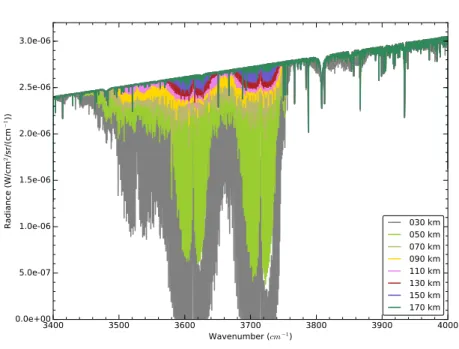
Figure 7 shows such a calculation in the IR, specifically in the 2.5-2.9 µm region for an arbitrary reference atmosphere extracted from the Mars Climate Database. The line-by-line transmittances were convolved with an approximate instrumental response at 0.15 cm-1 resolution, to mimic the NOMAD SO signal, as was done by Vandaele et al., 2015 [132] in similar transmittance calculations but at tangent heights below 50 km. Using a conservative estimation of the SNR of 2500 for the SO channel (Robert et al., 2016 [112]), consistent with the NESR value shown in Table 1, all the spectral features visible in figure 7, even at 170 km altitude(about 0.05 nbar in this reference atmosphere), should be detected in the SO signal. Since the ACS MIR has a spectral resolution about 3 times better than the SO channel but a lower sensitivity by about the same factor, the same conclusion applies to the solar occultation with ACS/MIR.
Figure 8 shows that these sensitivity levels are excellent to detect “hot bands” of CO2; the First Hot band of the major isotope (626) in particular should be
clearly seen at altitudes well above 130 km (at least up to about 150 km, or
equivalently to CO2 number densities around 1010 cm−3, for this model
atmo-sphere and the assumed SNR value). This is very interesting for non-local ther-modynamic equilibrium studies (non-LTE). Emission spectroscopy is very useful to study the excited states of molecules like CO2 which may present strong
3400 3500 3600 3700 3800 3900 4000 Wavenumber (cm−1) 0.0e+00 5.0e-07 1.0e-06 1.5e-06 2.0e-06 2.5e-06 3.0e-06 Ra dia nc e ( W/ cm 2/sr /(c m − 1)) 030 km 050 km 070 km 090 km 110 km 130 km 150 km 170 km
Fig. 7 Simulation of the solar radiance expected in the NOMAD LNO and ACS MIR channels at different tangent altitudes, as indicated, and for a typical Martian reference atmosphere.
rate coefficients poorly constrained in laboratory and which therefore require as-sumptions and approximations (L´opez-Valverde and L´opez-Puertas, 1994a [83]; L´opez-Puertas and Taylor, 2001 [80]). Absorption spectroscopy, on the contrary, sounds the lower state of the transitions and is more free from those modeling un-certainties. The lower state is the ground state in the fundamental bands, but for hot bands it is an excited state. Figure 8 shows LTE-NLTE differences of simulated transmittances to illustrate how the NOMAD SO measurements should permit the study of the population of the lower state of the First Hot band, the (010) state. This is expected to separate from LTE in the upper mesosphere and the whole thermosphere during daytime (L´opez-Valverde and L´opez-Puertas, 1994b [82]), and these data combined with the total density of CO2 would supply a direct
measurement of the (010) state population, a direct test for the non-LTE
mod-els. Let us recall that these models supply one of the two key ingredients of the
Martian radiative balance at thermospheric altitudes, i.e., the thermal cooling at 15-µm, the other one being the EUV solar heating mentioned in section 2.
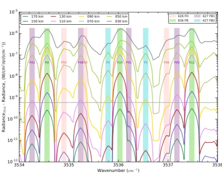
Figure 9 shows this detection capability more clearly in a narrow region around 2.83 µm, where the CO2-636 isotope has its strongest absorption lines. In this figure
the irradiance shown is not the actual flux level observed but the difference from the flux at the top of the atmosphere (TOA). Individual lines from diverse CO2
bands and isotopes show a funny shape due to the log scale used. If the expected noise level is confirmed, the isotopic 636 lines should be detected below about 150
3450 3500 3550 3600 3650 3700 3750 3800 Wavenumber (cm−1) −0.005 −0.004 −0.003 −0.002 −0.001 0.000 0.001 Tra nsm itt an ce di ffe ren ce (L TE -NL TE ) 636 FH bands 626 FH bands
Fig. 8 Simulation of the atmospheric transmittance differences LTE-NLTE by the “First Hot” (FH) band of the two main CO2isotopes, 626 and 636, as indicated, at a tangent altitude of
130 km for the reference atmosphere used in this work. A line for a SNR=5000 is indicated for reference. See text for details.
km. We can also see lines of the First Hot (FH) band of the main CO2 isotope
(626) in the upper mesosphere and below.
Other CO2 and CO ro-vibrational bands in the near-IR range [1.0-2.0] µm,
which can be covered by the ACS-NIR instrument will also be useful for sounding although up to lower altitudes. The strongest CO2 band in this range, at 1.43
µm, about 1000 times weaker than the 2.7 µ bands, was used to derive CO2 up
to 90 km by Fedorova et al., 2009 [35] during solar occultations with SPICAM. Similar or higher altitudes should be achieved with NIR, given its better SNR and spectral resolution . The interest of using this band is the simultaneous derivation of H2O from the nearby band at 1.38 µ, as exploited by SPICAM ( Fedorova et
al., 2009 [35]. The CO overtone band at 2.3 µm could be detected in single CO measurements by NOMAD and ACS at least below about 75 km under dust free conditions, with one single solar occultation, and perhaps up to the mesopause (Korablev et al., 2017 [72]. Also its fundamental at 4.7 µm band could be detected up to the lower thermosphere with TIRVIM during solar occultation. These are estimates extrapolating the sensitivity study of the NOMAD IR channels at 20 km tangent height by Robert et al., 2016 [112].
Further in the IR region, other molecules like nitric oxide have emission bands, at 5.3 and 7.6 µm, which should also be detected in solar occultation with TIRVIM. For details of the TIRVIM detection limits for different species we refer the reader to the companion paper by Korablev et al., 2017 [72] in this issue.
3534 3535 3536 3537 3538 Wavenumber (cm−1) 10-12 10-11 10-10 10-9 10-8 10-7 10-6 10-5 Ra dia nc eTOA - R ad ian cez (W /cm 2/sr /(c m − 1)) P48 P49 P50 R8 P42 R10 P41 P40 R12 P43 P4 P3 170 km 150 km 130 km110 km 090 km070 km 050 km030 km 626 FH636 FB 627 FB1627 FB2
Fig. 9 Simulation of the difference between the solar spectral irradiance at each tangent altitude and that at TOA. Different colors are used to visualize the different tangent altitudes. The gray line is the nominal noise of the NOMAD SO channel. Positions of individual lines and bands are indicated with arrows. “FH” and “FB” stand for First Hot and Fundamental Bands. See text for details.
Atmospheric thermal structure Atmospheric temperature profiles can also be ob-tained from the scale height of the species densities. Examples of similar studies using limb observations are the analysis of SPICAM stellar occultations in the UV by Forget et al. (2007) [38] and the retrieval of the Venus thermal structure from SPICAV stellar occultations (Piccialli et al., 2015 [109]) and from SOIR solar occultations (Mahieux et al., 2010 [92], Mahieux et al., 2015a [90]). The spectral resolution might not be enough to derive atmospheric temperatures directly from the rotational distribution of all the bands, although this was possible with SOIR on board Venus Express (VEx) in a few cases (Mahieux et al.,2015 [91]). Given the similarity and heritage between NOMAD and SOIR, and despite the different FOV and integration times, similar vertical resolution in the temperature retrieval is expected,which means close to the sampling, i.e., about 1 km for integration times of 1 s (Vandaele et al., 2017 [131]).
3.1.2 NOMAD UVIS channel
In the UV part of the spectrum, 200-650 nm, the solar occultation with UVIS is expected to map ozone and aerosols, as has been done with SPICAM similar observations in the past (M¨a¨att¨anen et al., 2013 [86]). Both ozone and aerosols have indirect implications for the upper atmosphere, via photochemistry and radiation.
Fig. 10 The vertical distribution of ozone as a function of the solar zenith angle (SZA) simulated by the LMD Mars global climate model for a chosen solar occultation by SPICAM. Three lines-of-sight with tangent altitudes of 20, 30 and 40 km of the SPICAM occultation are overplotted with symbols (yellow, red and blue crosses). The color scale goes from 0 to 8×10¹⁴m−3. The colors of the crosses in the lines-of-sight do not follow the abundance’s color
scale; they are simply fixed for clarity.
Ozone Ozone has been profiled in the Martian atmosphere up to the altitude of 50 km by SPICAM on board Mars Express (Lebonnois et al. 2006 [75], Montmessin and Lef`evre, 2013 [99]). These measurements were performed by stellar occultation at night, when ozone has a long photochemical lifetime and can be reasonably as-sumed to be horizontally uniform. The situation is different during the day, when ozone is photolyzed by solar radiation with a timescale shorter than five minutes. As in the Earth mesosphere, daytime ozone concentrations are therefore expected to be much smaller than during the night. The amplitude of the day-night differ-ence depends on the rate at which the ozone that is lost by photolysis is reformed by the reaction of oxygen atoms with molecular oxygen. The efficiency of this three-body process decreases rapidly with altitude. Thus, the strongest day-night differences in ozone are expected in the middle and upper atmosphere of Mars. At those altitudes, this leads to clearly heterogeneous ozone concentration for an ob-servation performed across the terminator. The classical vertical inversion methods (so-called onion-peeling) make the hypothesis that the atmospheric composition is spherically symmetric, which fails in this case.
Figure 10 shows the vertical distribution of ozone as modeled by the photoche-mistry-coupled Mars LMD GCM. Here the results have been calculated with the one-dimensional version of the GCM to acquire a fine description of the ozone vari-ation with solar zenith angle around the terminator. We have included in the figure
crosses) illustrating the path integrated during the observation. Notice that this type of inertial pointing is not within the TGO nominal solar occultation modes, although it could be performed. Figure 10 demonstrates the clear deviation of the atmosphere from the spherical symmetry due to the day-night gradient mentioned above, and the way solar occultations probe very different ozone concentrations along the line of sight.
In such a case, when comparing solar occultation observations to a model, the most straightforward method is to extract from the model the slant profiles cal-culated along the observational lines-of-sight, which ensures that the quantities are comparable since they have been acquired in the same way. If local vertical profiles are to be compared, the hypothesis of the spherical symmetry in the inver-sion method would need to be circumvented by accounting for the gradients in the atmosphere around the terminator, at least for the photochemically active species (i.e., ozone), but in the optimal case also for the full atmospheric structure. Aerosols Small particles seem to be frequent at high altitudes. Particles of effective radius close to about 1 µm have been observed by the VIRTIS and SPICAV/SOIR instruments in the Venus upper mesosphere up to 90 km during nighttime and twilight (Wilquet et al., 2009 [136], deKok et al., 2011 [26]) and scattering during daytime was observed at 4.7 µm to be much stronger than the non-LTE fluores-cence of CO up to 100 km tangent heights (Gilli et al., 2015 [50]). Using Venus as a guide, the upper limit in atmospheric pressure where scattering can be observed would correspond in the Martian atmosphere to the vertical region around 60 km. In Mars, dust detached layers with similar particle sizes have been observed with TES and MCS up to 40 km in the tropical region (Guzewich et al., 2013 [58]; Heavens et al., 2014 [60]), with TES limb data during dust storms up to 60 km (Clancy et al., 2010 [21]), and with TES up to 65 km, forming what has been named “upper dust maximum” (UDM), centered at 45-65km during daytime in the summer season in the Northern hemisphere (Guzewich et al., 2013 [58]). Also mesoscale simulations of energetic convection within dust storms suggest effective injection of particles up to 50 km (Spiga et al., 2013 [120]). The expected decrease of particles size with altitude grants the abundance of smaller particles up to much higher in Mars. Indeed there are several direct detections of aerosols at mesospheric altitudes, precisely with solar occultations in the UV with SPICAM/Mars Express (M¨a¨att¨anen et al., 2013 [86]). They found frequent high aerosols layers between 55-70 km, even at 90 km altitude, with typical vertical extensions between 10 and 20 km, although apparently not reaching the uppermost mesosphere 100−120 km. The mesospheric aerosol layers seemed to be located at higher altitudes in the Southern hemisphere. These aerosols seemed to be associated to a large dust con-tent at lower altitudes, during global dust storms, which possibly lofted particles up to those heights for an extended period of time, but very often they had the form of detached layers of shorter duration, outside large dust loading in the lower atmosphere.
The separation of dust and ice aerosols is another important goal that may be achieved combining UV and IR channels (UVIS and SO/MIR) during solar occultation. The above mentioned study of the SPICAM solar occultation mea-surements in the UV (M¨a¨att¨anen et al., 2013 [86]) did not resolve the nature of the aerosol layers studied but suggested that many of the high altitude aerosols
might more likely be formed by water condensation than lifting of dust particles. The use of three solar occultation channels ranging from the UV to the IR has been exploited in the case of Venus to detect and retrieve distinct particles popu-lations of three different radius (Wilquet et al., 2009 [136]). Further, the combina-tion of particle radius and optical thickness variacombina-tions within a detached aerosol layer could discriminate between dust and ice particles (Montmessin et al., 2006 [100]; M¨a¨att¨anen et al., 2013 [86]). An interesting result from the combination of SPICAM UV and IR solar occultations during the Northern winter, obtained by Fedorova et al. (2014) [36], is the identification of a bi-modal distribution of particles on Mars at tropospheric altitudes (10-40 km). The coarser mode, with particle radius near 1 µm was consistent with many previous atmospheric dust observations, and seemed to contain both dust and H2O ice particles, with 0.7
and 1.2 µm radii, respectively. But their UV data were essential to identify the fine mode, with radius smaller than 0.1 µm and reaching altitudes up to about 60-70 km in such a data sample.
In summary, the UVIS channel may extend significantly the upper atmospheric dataset of aerosols, clarifying the population and variability of small particles during periods of large dust storms and other episodes, and if combined with a concomitant IR sounding and microphysical models, clarify the nature of the aerosol layers.
3.2 Nadir mapping
3.2.1 Infrared mapping with LNO and TIRVIM
The recent exploitation of non-LTE nadir data from VIRTIS/Venus Express by Peralta et al. (2016) [107] shows that it is possible to map the upper atmosphere not only with the classical limb sounding but also in nadir geometry, if the signal is sufficiently optically thick. This is the case of the strongest CO2 band in the
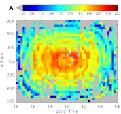
IR, the 4.3 µm band system, in the case of Mars and Venus. Figure 11 shows the map of thermospheric temperatures obtained on Venus, combining very sparse data from VIRTIS during the Venus Express mission. The altitude range sampled is wide, between 100 and 150 km, and the temperatures show a global view not far from model expectations (examined at the same altitudes), except for a systematic cold bias compared to the simulations. No similar maps exist on Mars and ACS offers an opportunity for a routine mapping of thermospheric temperatures from a proper analysis of this signal.
We explored the possibility of similar sounding at other wavelengths, but the situation is not as good as in the 4.3 µm band. Figure 12 shows the calculations for the CO22.7 µm band system in a nadir geometry, as observed by the NOMAD
LNO channel. This CO2band might be the second best candidate for such a
map-ping. The non-LTE enhancement is significant, compared to the LTE calculations, but the emission, even after spectral summation of the complete band, is about two orders of magnitude lower than the expected noise level (Table 1). Averaging of large amount of data may build up a signal but at the expense of temporal resolution. This is not a big issue in Venus, whose thermospheric structure seems more linked to the local time, but it is a serious difficulty for Mars, whose upper
Fig. 11 Map of Dayside thermospheric temperatures in Venus retrieved from nadir observa-tions of the non-LTE 4.3 µm emission by VIRTIS-H/Venus Express. After Peralta et al., 2016 [107]
atmosphere seems to be much more dynamic and variable (Piccialli et al., 2016 [108]).
3.2.2 Ultraviolet mapping with UVIS
The continuous UV mapping in nadir will supply a useful dataset to study airglow. The nightglow signals will be weaker than the limb components and than solar occultation detections but the accumulation of data may reveal the emissions and permit analysis of the spatial and temporal variations. One notable example is the NO nightglow, detected in the limb but not in nadir by SPICAM (Bertaux et al., 2005 [5]). This is an emission of large interest as it is associated to downwelling of atomic species (O3P
and N4
S) from the global interhemispheric circulation during solstices (Bertaux et al., 2005[5], Stiepen et al., 2015 [125]). However, there are discrepancies between models and simulations at equatorial latitudes, where such emissions are expected to be much weaker (Gagn´e et al., 2013 [42]). In addition, there is a remarkable variability observed with SPICAM in the peak emission, which seems to be located between 70 and 85 km altitude but does not show any clear correlation with latitude, local time, magnetic field, or solar activity (Cox et al., 2008 [25]). Recently, nadir observations with IUVS on board MAVEN were combined into quasi-global maps of the NO nightglow revealing an unexpect-edly complex structure (Stiepen et al., 2017 [126]). In addition to inhomogeneous brightening near the limb, a general intensification is observed surrounding the
Fig. 12 Simulation of the near-IR emission level in the center of the intense 2.7 µm bands of CO2 during a nadir observation. Red lines: non-LTE daytime emission; green line: LTE
calculation.Bottom panel: difference between the non-LTE and the LTE spectra.
winter pole. Streaks and spots extending toward lower latitudes suggest the pres-ence of irregularities in the wind circulation pattern. Regarding dayglow emissions above 200 nm, these are surely very hard to detect at the nadir due to the strong signal from scattered solar radiation. The best chance to study them would be at the limb (see below).
4 Additional capabilities 4.1 TGO Aerobraking Phase
Spacecraft aerobraking maneuvers have traditionally been exploited for in-situ sounding at very high altitudes in an atmosphere. Accelerometer data during spacecraft deceleration by atmospheric drag can directly supply along-track densi-ties, and infer vertical profiles of densities and temperatures with the help of model assumptions or hydrostatic approximation (M¨uller-Wodarg et al., 2016 [102]). In Mars, aerobraking has been performed during three NASA orbiters, Mars Global Surveyor, Mars Odyssey and Mars Reconnaissance Orbiter (Keating et al., 1998 [67], Withers et al., 2003 [140], Wang et al., 2006 [135], Bougher et al., 2006 [8], Moudden et al., 2010 [101]), and has supplied unique insights into the thermo-spheric dynamics and the links between lower and upper atmothermo-spheric regions (see Zurek et al., 2015 [147], Bougher et. al, 2017 [9], and references therein). Also, al-though MAVEN did not use aerobraking, it does detect atmospheric drag during
Fig. 13 Expected evolution of the periapsis’ altitude during a preliminary version of the TGO aerobraking period (see text). The colors indicate the solar zenith angle at the periapsis location, as indicated in the top scale; values above 90◦normally correspond to nighttime.
Fig. 14 Expected evolution of the periapsis’ latitude during the whole aerobraking period. As in 13 the colors indicate the solar zenith angle. The upper and lower lines show the locations where the spacecraft crosses (enters below) the 200 km reference altitude.
its orbit, specially during the deep dips into the lower thermosphere, which need to be exploited (Jakosky et al., 2015 [63], Bougher et. al, 2015 [7], Zurek et al., 2015 [147], Zurek et al., 2017 [146]). ESA, on the other hand, has performed only one aerobraking campaign, during the last phase of the Venus Express mission. These operations permitted successful retrievals of density profiles which revealed wave phenomena in polar regions (M¨uller-Wodarg et al., 2016 [102]) and permitted comparisons with atmospheric reference models (Bruinsma et al., 2015 [13]).
The aerobraking phase of Exomars TGO will supply an additional source of information on the still highly incomplete dataset of in-situ thermospheric densities and temperatures available to date. A large interest in the TGO dataset comes
from the combination of three factors: a wide latitudinal coverage, an extended investigation in time, and a focus on the lower thermospheric altitudes. Starting with the last one, the expected altitude range of the periapsis is [100-120] km, with some seasons at higher altitudes [150-160km], as shown in Figure 13. This is a prediction based on a preliminary estimate of the aerobraking period, extending from Jan-Nov 2017, available at the time of writing this article, and valid for us to illustrate some aspects. It will obviously depend also on the performance of the aerobraking which will be monitored on a daily basis. According to this prediction, the latitude range that could be explored during the aerobraking phase in the TGO’s nearly-polar orbit goes up to 74◦S, as shown in Figure 14. The aerobraking
phase will be executed during a very extended and continuous period of time, of at least up to 9 months, covering a seasonal range Ls ≈ 300◦− 90◦. As Figure 14 shows, in the first months it will probe the dayside of the planet, then move toward the dark side as the orbital period gets shorter. The part of the orbit when the spacecraft will be below 200km altitude will cover around 40 deg in latitude, until TGO orbit achieves its final circular shape at 400 km above the planet’s surface. It will have a periodicity of 1 Martian day (sol) at the beginning and 2 h at the end of the aerobraking experiment.
One of the open problems whose study could benefit from the TGO aerobrak-ing data is the propagation of gravity waves. Previous analysis usaerobrak-ing extended aerobraking datasets from MGS and Mars Odyssey suggest that such a propa-gation is possible up to the lower thermosphere, and might be filtered by tidal activity (Withers et al., 2006 [139]). Also non-migrating tides were detected in the aerobraking data (Wang et al., 2006 [135], Fritts et al., 2006 [41]), together with smaller scale perturbations without a clear oscillatory shape and which remain unexplained. The extended aerobraking during both day and night, including high southern latitudes, should supply new insights into these dynamical phenomena.
The combination of the aerobraking results and of the regular solar occultation data from NOMAD and ACS later in the mission also offers interesting opportu-nities; in particular, combining total density from aerobraking and CO2 densities
from solar occultation can yield constraints on CO2mixing ratios at thermospheric
altitudes, as has recently been exploited for Venus (Limaye et al., 2017 [78]).
4.2 Limb emissions off-the-terminator
We mentioned above the two major pointing modes of NOMAD and ACS, i.e., solar occultation and nadir mapping. However, there exists the possibility to perform also limb pointing with the LNO channel given its flip mirror (Neefs et al., 2015 [105]), and similarly, it is possible to perform limb observations with the TIRVIM and NIR channels by moving the nadir boresight (Korablev et al., 2017 [72]). The UVIS channel could also be operative in a limb viewing mode, co-aligned with the LNO signal. We describe four possible TGO configurations to perform a limb sounding off-the-terminator (LSoffT, in short), considering the NOMAD and ACS optical layouts.
– LSoffT #1. Limb pointing using NOMAD flip mirror. During regular nadir mapping, the NOMAD LNO slit is oriented across-track and its pointing could be changed to a limb pointing using the on-board flip mirror. Consequently the
pendicular to the limb) and centered at an altitude of about 67 km above the ground at the tangent, i.e., viewing altitudes between 35 and 110 km. Binning of the “spatial pixels” is possible, which will enhance the limb detection. In this configuration only the NOMAD LNO and UVIS channels would perform a limb observation, not the ACS channels.
– LSoffT #2. Inertial limb scan. If possible, this will be an emulation of a solar occultation sequence but off-the-terminator, i.e., the spacecraft maintains a fixed attitude (in the solar system’s reference frame), but is not pointing to the Sun. The NOMAD and ACS fields of view move across the limb due to the spacecraft’s orbital motion, effecting a limb scan. Signals from the SO, UVIS and MIR channels would be available, but the SO should be replaced by the LNO to improve sensitivity. Both the dayside and the nightside of the planet could be explored. The LNO slit would be perpendicular to the limb; this is not the ideal configuration to maximize the detection of weak emissions but it has the advantage of performing a nearly simultaneous sampling of the emissions over a wide range of altitudes (centered at 67 km if exactly perpendicular). The NIR channel can also be used in this configuration, in this case, its orientation is nearly perpendicular to the LNO slit, i.e., well positioned for spatial addition to increase detectability.
– LSoffT #3. Nadir boresight slew. By rotating the spacecraft around its along-track (Z) axis the boresight (-Y) axis would perform an effective limb sound-ing, with all NOMAD and ACS instruments operating in their regular “nadir mode”. Simultaneous signals from LNO, UVIS, NIR and TIRVIM would be available in this configuration. Attention should be given to the likely reduced pointing accuracy during such a slew maneuver, and the large fields of view of some of these channels (we will discuss these below).
– LSoffT #4. Fixed limb tracking. After the simple inertial limb scan (LSoffT#2) and/or the nadir boresight slew (LSoffT#3) have been tried, a next step would be to position the spectrometer slit across the limb to perform a fixed limb tracking, that is to keep the slit pointed at a fixed tangent altitude above the planet as the spacecraft moves through its orbit. This allows a truly 2D map of limb emissions to be built up, and permits also long integration of faint sources. A similar strategy was used on Venus Express to search for oxygen airglow (Migliorini et al., 2013 [97]). Both, the solar occultation channels (as in LSoffT#2) or the more sensitive nadir ports (as in LSoffT#3) could be used. Notice that LSoffT#1 also represents a limb tracking but at the fixed tangent altitude of 67 km above the surface and using only two NOMAD channels. These non-standard observational configurations would add new ways of ex-ploiting the TGO science, and therefore, we recommend its use during short upper atmosphere campaigns. We mention next several of the scientific goals inherent to these LSoffT modes which, if confirmed with observations, would represent valu-able and added science. Some of them are of a general character and require specific examination, but all merit their execution and testing. The first one is the building of vertical profiles of minor species and dust outside the very peculiar region at the day/night terminator. Also, these observations shall permit to complete the daily
cycle of minor species (chemistry & dynamics) outside the specific local times of the terminator at each latitude. Specific emission from solar fluorescence and air-glow data would permit to study the upper atmosphere physics behind them, and perhaps to derive information about the thermal structure in the vertical. After detection of specific areas on the planet where trace gases are found, a vertical sounding capability above such areas would be of large interest, if their emission in a limb geometry permit to gain insight into their vertical distribution. These observations would also extend in time the current database of Mars limb observa-tions to date (OMEGA, PFS and SPICAM on Mars Express, TES on MGS, and MCS and CRISM on board MRO).
In addition, there could be defined a number of moments during the mission for specific new targets which shall require these observing modes. Four examples are (i) the search for very high altitude clouds, airglow and aurora phenomena, (ii) the investigation of the thermal structure in very-high-latitude regions and its daily cycle,(iii) 2D mapping of emissions and densities using the limb-tracking modes, which could depict the propagation of gravity waves, and (iv) broad spectroscopic searches from the UV to the IR at these altitudes, opening a window for serendipity science. Some of these are expanded in more detail next. In summary, we anticipate that both NOMAD & ACS will increase their scientific impact thanks to these LSoffT observation modes.
4.2.1 Nightglow
Mars aurora The Martian aurora, observed for the first time with SPICAM/MEx (Bertaux et al., 2005 [6]), was sporadic, associated to magnetic anomalies in the crust, and peaked at about 135 km. Later, a different kind of aurora, diffuse, quasi-global and down to 60 km altitude, was observed with IUVS/MAVEN during periods of strong solar activity (Schneider et al., 2015 [115]). Martian auroras have triggered renewed interest in the Martian upper atmospheric emissions as probes of the thermospheric structure and as validation tools for models (Gagn´e et al., 2013 [42]; Gerard et al, 2015 [47]; Soret et al, 2016 [119]).
The SPICAM observations show prominent UV emissions from the CO (a3
Π− X1Σ) Cameron Bands (190-270 nm), the CO2+ doublet around 289 nm, and the
atomic oxygen 297.2 nm trans-auroral line. Figure 15 shows the vertical intensity profiles from the CO Cameron and the CO2+ doublet observed with SPICAM
and studied by Soret et al., 2016 [119], who could reproduce the altitudes of the auroral emissions with a Monte-Carlo model of electron transport in the Martian thermosphere. The diffuse aurora shows similar spectral features but with lower intensity levels and peak altitudes (Schneider et al., 2015 [115]).
UVIS should combine nadir and limb emission observations to study the in-tensity and the spatial distribution of the auroral emissions, with attention to the residual magnetic field regions and to strong solar events. Recently, Lilensten et al. (2015) [77] suggested that during strong solar events there could be auroral emissions in the visible, possibly localized as well, including the red and green lines of atomic oxygen and the CO2+ Fox-Duffenbach-Barker (FDB) bands in the
blue-visible spectral region. The UVIS channel offers possibilities to detect such events. A specific limb inertial mode in the nightside hemisphere during such solar conditions would be most adequate for such a study.
Fig. 15 Vertical profiles of UV auroral emission in Mars, observed with SPICAM. After Soret et al., 2016 [119], with permission. Notice that these are apparent limb profiles, before correction for the non spherical symmetry of the discrete aurora; the actual peak emissions occur around 120-130 km.
O2 IR Atmospheric bands at 1.27 µm The O2 IR airglow at 1.27 µm has been
extensively studied in Venus using ground based telescopes and spectral images at the nadir and limb obtained with the VIRTIS spectral imager on board Venus Express. Its detection in the Mars nightglow spectrum is much more recent. The first detection was made with the OMEGA instrument on board Mars Express (Bertaux et al., 2012 [4]). This emission was further investigated and its seasonal variations were characterized with CRISM on board the MRO satellite (Clancy et al., 2012 [17]) and SPICAM IR on Mars Express (Fedorova et al., 2012 [34]). Detections were made close to the southern and northern poles during polar night. This nightglow layer is produced by three-body recombination at 40-50 km of oxy-gen atoms produced on the dayside by CO2 dissociation and transported to the
polar dark regions by the global circulation. The intensity observed by CRISM at the limb reaches about 14 Megarayleighs (MR), a brightness that should be mea-surable with the NIR/ACS channel. Comparisons with GCM predictions (Gagn´e et al., 2013 [42]) indicate that the model underestimates the high latitude O2
airglow brightness by a significant margin. Although high latitude measurements will be limited by the TGO orbital inclination, the mid-latitude brightness near equinox may be observed and the O density derived from these observations. Un-fortunately, the altitude range where this derivation is possible does not cover the upper mesosphere and lower thermosphere. This is the region where the strongest
CO2 emissions at 15-µm occur and depend most on the collisional exchanges
be-tween atomic oxygen and CO2; and this is the process which together with the
EUV heating mentioned in section 2 dominates the energy balance of the Mars