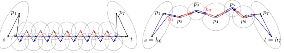
Collaborative Delivery with Energy-Constrained Mobile Robots
Texte intégral
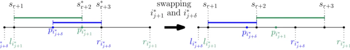
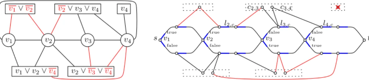
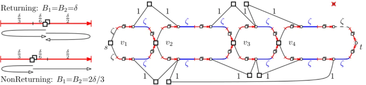
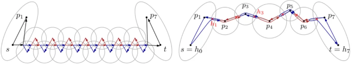
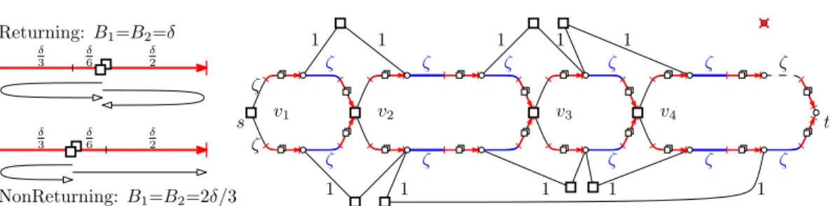
Figure

Documents relatifs
ﺍﻟﻤﻁﻠﺏ ﺍﻟﺜﺎﻨﻲ :ﺁﺜﺎﺭ ﺍﺴﺘﻌﻤﺎل ﺍﻟﺩﻋﻭﻯ ﻏﻴﺭ ﺍﻟﻤﺒﺎﺸﺭﺓ : ﺴﺒﻕ ﻭ ﻗﻠﻨﺎ ﺃﻥ ﺍﻟﻐﺭﺽ ﻤﻥ ﺍﻟﺩﻋﻭﻯ ﻏﻴﺭ ﺍﻟﻤﺒﺎﺸﺭﺓ ﻫﻭ ﺍﻟﻤﺤﺎﻓﻅﺔ ﻋﻠﻰ ﺍﻟﻀﻤﺎﻥ ﺍﻟﻌﺎﻡ ﻭ ﺃﻥ ﺍﻟﺩﺍﺌﻥ ﻋﻨﺩ
Existing models on the IRP are mainly divided into two categories: one with continuous time, constant demand rate and infinite time horizon, typically the case of the Cyclic
Flow and energy based satisfiability tests for the Continuous Energy-Constrained Scheduling Problem with concave piecewise linear functions.. Doctoral Program, 21th
Below we recall a number of previous results, which, as we shall argue in the following section, provide much insight into the structure of 1 and 2-connected AP graphs, and
Keywords: Condition number, Resolvent, Toeplitz matrix, Model matrix, Blaschke product 2010 Mathematics Subject Classification: Primary: 15A60;
Indeed, [4] proved Theorem 1.10 using standard rim hook tableaux instead of character evaluations, though virtually every application of their result uses the
In order to do so, compare the free energy of a perfectly ordered system with the free energy of a partially disordered case that introduces the less energetic frustrations
This talk will provide an overview of this new challenging area of research, by analyzing empathy in the social relations established between humans and social agents (virtual
