Client Segmentation Under Real-World Constraints
by Gregory Young
B.S. EECS, Economics MIT, 2017
Submitted to the
Department of Electrical Engineering and Computer Science In Partial Fulfillment of the Requirements for the Degree of
Master of Engineering in Electrical Engineering and Computer Science
at the
Massachusetts Institute of Technology
June, 2018
© 2018 Massachusetts Institute of Technology. All rights reserved.
Author:
Department of Electrical Engineering and Computer Science May 25, 2018
Certified by:
Dr. Robert M. Freund, Professor, Sloan School of Management, Thesis Supervisor May 25, 2018
Certified by:
Sergei Lubensky, Director, First Republic Bank, Thesis Co-Supervisor May 25, 2018
Accepted by: _________________________________________________
Dr. Katrina LaCurts, Chairman, Masters of Engineering Thesis Committee
Signature redacted
Signature redacted
Client Segmentation Under Real-World Constraints by
Gregory Young
Submitted to the Department of Electrical Engineering and Computer Science May 25, 2018
In Partial Fulfillment of the Requirements for the Degree of Master of Engineering in Electrical Engineering and Computer Science
Abstract
Market segmentation is a very useful tool that can enhance knowledge of a firm’s customer base and therefore enable improved customer services and experiences that are more tailored to specific customer needs and preferences. Clustering is a natural and intuitive way to implement such segmentation, and in fact, there are a variety of standard methods by which to perform this. However, real-world considerations complicate its implementation, in particular, the necessity of not clustering in ways that could be considered discriminatory in terms of certain features such as gender or race. One way to mitigate such discriminatory clustering is through constraints that ensure that the clusters are balanced in terms of such features. However, such a clustering is barely, if at all, discussed in current literature. In this thesis, we develop and implement a new version of k-means clustering that is able to achieve comparable performance relative to an unconstrained clustering while at the same time address the constraints imposed by these discriminatory features.
Thesis Supervisor : Dr. Robert M. Freund, Professor, Sloan School of Management Thesis Co-Supervisor: Sergei Lubensky, Director, First Republic Bank
Acknowledgements
I would like to thank First Republic Bank and the MIT VI-A program for giving me this exciting opportunity. I enjoyed learning more about the banking industry as a whole, and it was very interesting to think about how I could reconcile my engineering knowledge with the real-world constraints and considerations that come with operating a bank.
There were many people that were instrumental to my work both at First Republic and at MIT. In particular, I would like to thank Sergei Lubensky, who served as my manager during my time at First Republic. Not only did he help me get acclimated to working at the bank, but he also was crucial in facilitating that reconciliation between engineering and real bank
considerations, given his unique position of having worked in banking for many years and being a former MIT student himself.
I also would like to thank Professor Robert Freund, who served as my thesis advisor at MIT. Despite our being on opposite sides of the country for a substantial part of this thesis work, he was very generous with his time and scheduling to allow us to meet over Skype on a regular basis. In addition, he provided valuable theoretical insight and questions that helped to drive the research in fresh and novel ways.
I also would like to thank Professor Duane Boning, who has been my academic advisor for the past four years. His guidance and insight into the undergraduate and M. Eng programs has been invaluable to my being able to take advantage of the many opportunities that MIT has offered over the years, ranging from studying abroad to a second major to the M. Eng program.
Finally, I would like to thank my friends and family for their invaluable patience and support, without which I would not be where I am today.
Contents
1 Introduction 8
1.1 Motivation . . . 8
1.2 Segmentation and Clustering . . . 10
1.3 Objectives and Caveats . . . 12
2 Research Project 15
2.1 Project Overview . . . 15
2.2 Data Gathering . . . 16
2.3 Algorithm Selection . . . 23
2.4 Similarity and Constraints . . . 27
2.5 Clustering Quality . . . 32 2.6 Terminating Clustering . . . 36 2.7 Algorithm Implementation . . . 37 3 Experiments 39 3.1 Experimental Dataset . . . 39 3.2 Data Standardization . . . 45 3.3 Behavior Check . . . 47 3.4 Anti-Discriminatory Clustering . . . 49 3.5 Batch Updates . . . 58
List of Figures
Figure 1: Clustering algorithm pseudocode
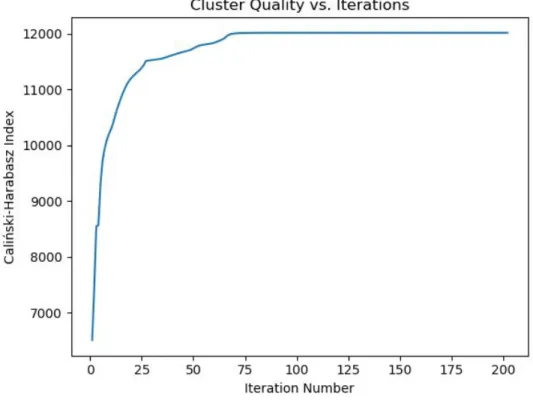
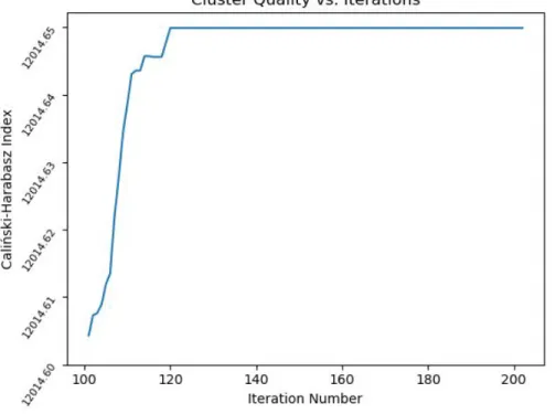
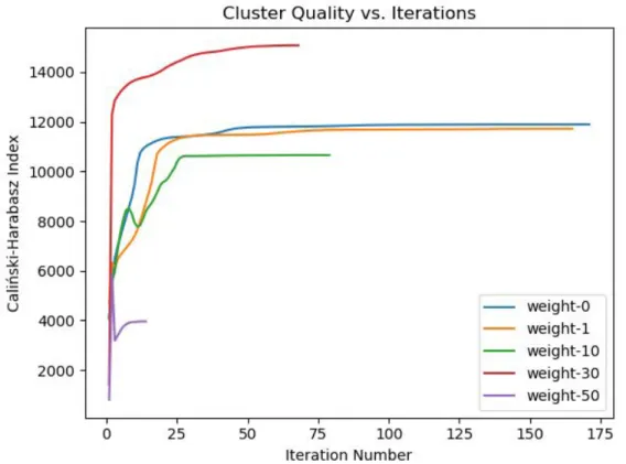
Figure 2: Cluster quality vs. iterations from our behavior check experiments
Figure 3: Same as Figure 2, except starting at iteration 100 Figure 4: Cluster quality vs. iterations from our anti-clustering
experiments using a Euclidean metric
Figure 5: Number of clusters vs. iterations from our anti-clustering experiments using a Euclidean metric
Figure 6: Degree of output separation vs. iterations from our anti-clustering experiments using a Euclidean metric
Figure 7: Degree of gender separation vs. iterations from our anti-clustering experiments using a Euclidean metric
Figure 8: Cluster quality vs. iterations from our anti-clustering experiments using the Kullback-Leibler divergence
Figure 9: Number of clusters vs. iterations from our anti-clustering experiments using the Kullback-Leibler divergence
Figure 10: Degree of output separation vs. iterations from our anti-clustering experiments using the Kullback-Leibler divergence
Figure 11: Degree of gender separation vs. iterations from our anti-clustering experiments using the Kullback-Leibler divergence
Figure 12: Cluster quality vs. iterations from our anti-clustering experiments using mini-batches
Figure 13: Number of clusters vs. iterations from our anti-clustering experiments using mini-batches
Figure 14: Degree of output separation vs. iterations from our anti-clustering experiments using mini-batches
Figure 15: Degree of gender separation vs. iterations from our anti-clustering experiments using mini-batches
List of Tables
Table 1: Client tenure summary and statistics
Table 2: Overall transaction counts and net transfers Table 3: Overall transaction counts and balances Table 4: Product account counts summary statistics Table 5: Product account balances summary statistics
Table 6: Category account counts and balances summary statistics Table 7: Client region counts
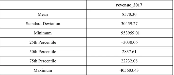
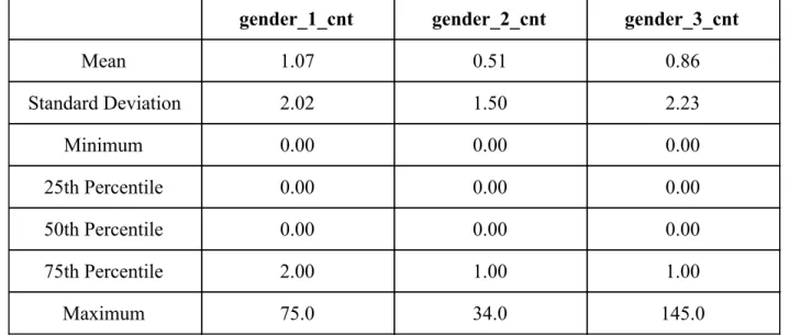
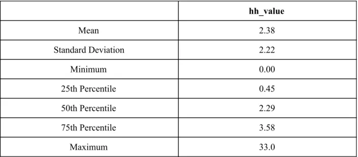
Table 8: 2017 revenue summary statistics Table 9: Gender count summary statistics Table 10: Output variable summary statistics
1. Introduction
1.1. Motivation
From a product perspective, the banking industry is not one of great differentiation. Although the exact terms and conditions may vary, the products and services offered from one bank to the next are very similar. Some examples include, but are not limited to, the following:
1) Checking accounts 2) Savings accounts 3) Loans & Mortgages 4) Online banking 5) Wealth management
Because of this similarity, banks must differentiate in another dimension: customer service and experience. Banks are very much customer-facing institutions by design, so performance in this dimension is absolutely vital to a bank’s success in the industry. Better service helps to improve customer loyalty, which can then translate into increased engagement with the bank (e.g. opening multiple accounts instead of just one) and additional customers through a customer’s personal network. Increased engagement can then translate into additional deposits for the bank, which can then be used to support a bank’s primary form of revenue generation: loans, where the revenue comes in part from the interest received on such loans.
For banks to provide an excellent customer experience, they need to understand the customers that they are serving. What are their needs and preferences? What are their likes and dislikes? Answers to these questions can then be used to tailor the banking experience for
customers to make it more enjoyable instead of inconvenient. An excellent example of this tailoring is the emergence of online banking, which even a half century ago was barely
conceivable. However, the rise of the Internet and the proliferation of smartphones, tablets, and similar technologies have made it a reality that walking over to an ATM or a branch is not necessarily as appealing when the large majority of a customer’s day-to-day activities is being conducted through these technological devices. By allowing customers to engage with banks via an online interface (i.e. a website or mobile application), they are able to more seamlessly engage with their bank instead of going out of their way to do so by finding the nearest ATM or branch.
It should also be noted that there is no one right answer to questions regarding customer tastes and preferences. In fact, to provide good customer service, those questions should be addressed at various levels of granularity. For example, the preference for using mobile or digital technologies is a national and international preference. However, more local preferences can be appealed to for example by enhancing branch decor to show support for local sports teams or partnering with nearby businesses to extend services unique to the surrounding area. From a customer point of view, the more needs and preferences that can be addressed, regardless of granularity, the more positively they will view their experience with the bank.
With different levels of customer preferences and needs to manage and update on a regular basis (customers are not static entities), the task of providing service and an experience that is well-tailored to the customer becomes more challenging. How do we know that we are addressing all of the relevant needs and preferences? How can we ensure that the provisioning of these tailored experiences is consistent from one banker to the next, between a branch and online? With thousands if not millions of customers to serve, and hundreds if not thousands of
bankers to manage to ensure consistent service, identifying and keeping track of customer needs and preferences quickly becomes unsustainable if performed manually. In addition, the process might be incomplete because there is simply too much data to process, meaning that insights could be overlooked to the detriment of the bank.
1.2. Segmentation and Clustering
The challenge of providing a tailored experience to customers is not a new problem. In fact, its implementation can be witnessed in many instances, whether it is the searches that Google returns to a user or the recommendations the Amazon provides to shoppers. Both are examples of ways in which companies attempt to customize the experience for each customer by relying on provided information and past interactions with the service to understand the customer that they are serving and to accommodate the service to their unique needs and preferences.
At the heart of this tailored experience lies a concept known as market segmentation, which can be defined as “the process of dividing the market into consumer groups [or clusters] with similar needs [and preferences]” (Lilien & Rangaswany, 1992). By performing this kind of segmentation of the customer base, we can use those insights to construct a profile, an
understanding that is, of all of the customers being served. With this profile, we are then able to provide the personalized experience and therefore the high level of customer service as desired.
Implicit in this definition of market segmentation is the fact that the segmentation process, at a high-level, has the useful property of being indifferent to the market to which it is being applied. From a bank’s perspective, this process can be applied to its customer base at varying levels of granularity. It could be used to segment the bank’s entire market of customers, but it could be used just as well with its market of college students or its market of customers
living in single-family residences. Thus, this segmentation could be used and applied in a variety of banking contexts and operations.
With the utility of market segmentation established, we must now identify a means by which to implement. A natural and intuitive way of doing this is clustering, which in its essence groups together objects that are most similar to one another. Similarity between objects is measured by the degree in which objects share features in common. For bank customers, features are characteristics that can be used to form an understanding of who they are and their needs and preferences. Features might include whether they own a smartphone, the type of residence they live in, and average annual salary. Although the similarity metric (or
measurement) is almost always numeric to facilitate comparison of similarity, the necessary requirement is that the set of all possible values for a given similarity metric is well-ordered (otherwise, similarity can’t be compared). In addition, for each feature, the similarity metric must be well-defined. This means that for all possible values x and y of that feature, the
expression must evaluate to a value . For the sake of simplicity, we will assume henceforth that is the set of all real numbers .
Similar to market segmentation, clustering is not a novel concept and has been a
well-known topic in research since the 1930s (Driver & Kroeber, 1932). In the intervening time, many different types of clustering algorithms have been developed. Some examples include, but are not limited to, the following:
1) K-Means Clustering 2) Hierarchical Clustering
Each of these algorithms groups together objects in different ways and has their own advantages and disadvantages, which will be expanded upon later in the thesis. In addition, this enumeration of clustering techniques does not include the fact that the similarity metric used to group together objects is parameterizable. Thus, when designing or choosing a clustering algorithm for a particular context, in addition to choosing the appropriate algorithm, the choice of similarity metric is also crucial and can come with trade-off considerations depending on the types of similarity metrics considered. Euclidean distance is often used, but that generally is appropriate for objects whose features are all continuous. Different metrics might be required if there are features that are not inherently numeric or that take on categorical values (Huang 1998). 1.3. Objectives and Caveats
Theoretically speaking, clustering is very effective at being able to identify groups of similar customers. However, this identification is not necessarily sufficient for our purposes. This segmentation of the customer base ultimately has a practical application: to provide insights to a bank about its customers that can then be used to provide improved and personalized service and experiences for them. Thus, in addition to generating clusters, our final clustering algorithm should produce clusters that are both intuitive and easy to act upon from the perspective of business operations. More specifically, the clusters should:
1) have simple and intuitive descriptions that are easy to ascertain 2) should rely on quantities that are straightforward to measure, and 3) should provide robust actionable insight and strategic value.
The first and second requirements are important for the purposes of intuition. The more transparent the inputs and outputs are, the easier it is to understand how the clustering works, as it will be clearer as to which features the clustering is using to group together customers. This level of transparency, in addition to being useful from an auditing perspective, will be useful for those who will receive and act upon the results produced from the clusters: executives and bankers themselves, neither of whom will necessarily have been intimately involved with the design and details of the algorithm. Providing this kind of clarity to the end-user would facilitate buy-in, which is needed if the algorithm is to have practical value for the bank.
The third requirement addresses the need for the results to be actionable. That is, the results should in part provide valuable and tangible insights that the bank can use to provide improved customer service and experience and thereby encourage further engagement with the bank. Given the stakes, it is therefore important that any results achieved have not been
discovered purely by chance or by imposing numerous assumptions. Ideally, the insights found should be reproducible using as few assumptions as possible so that the conditions used to generate those insights are as close to reality as possible.
Another aspect to this robustness is that using this algorithm to cluster and group together customers is not a one-time event. Customer needs and preferences are constantly changing. The business contexts in which this clustering might be needed can vary. Thus, for the clustering algorithm to be of long-term strategic value to a bank, not only should the insights generated by the algorithm be capable of use for an extended period of time, but by design of the clustering itself, the algorithm should be adaptable to generate useful insights given varying inputs about a bank’s customers or a subset thereof.
Finally, as alluded to at the beginning of the discussion for this third requirement,
actionable insights are not solely about providing tangible business insight and direction. Banks are subject to regulatory oversight and thus must be mindful of said regulations when providing service to customers. Ultimately, when performing clustering for the purposes of market segmentation, it will result in the differentiation of services provided depending on needs and preferences. However, care must be taken to ensure that such differentiation is not considered discriminatory. For example, if those services pertained to lending, the Equal Credit Opportunity Act prohibits differentiation based on demographics such as race, sex, age, national origin and marital status (Federal Deposit Insurance Corporation, 2018).
Given that clustering is about grouping together objects based on similarities in features, these regulatory constraints do in part conflict with this purpose. To protect against potential regulatory violations, we should explicitly try to avoid clustering on demographic features such as sex and age. However, it is not sufficient to simply exclude them from consideration during clustering. If the produced clusters happen to exhibit any significant demographic bias, it could be risky to act upon these clustering results because of the potential regulatory violations. Thus, in order to alleviate this concern, the clustering should in fact explicitly discourage these kinds of biases. For example, any clusters produced could undergo an adjustment process to ensure that they are balanced across demographic features. Regardless of implementation, the fact is we are doing a kind of anti-clustering over these features with this explicit discouragement. Combined with the necessity of intuition and practical use, regulatory requirements complicate the
implementation and adaptation of clustering (and market segmentation for that matter) in the context of banking and customer service, and we focus on these complications in this research.
2. Research Project
2.1. Project Overview
The research for this paper was conducted in collaboration with First Republic Bank (FRB), an American bank and wealth management company based in San Francisco that has been in operation since 1985. At FRB, customer service is paramount. It is evidenced by their slogan, “It’s a privilege to serve you,” and one of the core values at the bank is to provide extraordinary service (First Republic Bank, 2018). Although financial profitability is also very important, their philosophy is that this business end goal is best achieved through “hard work and exceptional client service” (First Republic Bank, 2018).
Given the level of importance that FRB places on customer service, it is understandable that this kind of research would be of great interest to the bank to continue and grow what has arguably been a very successful approach to banking operations. For example, according to their April 13th, 2018 8-K form filing (this is filed with the U.S. Securities and Exchange Commission to convey any tangible business changes that could be of importance to shareholders), net
income rose year-over-year by 12.6%. In addition, from January 2014 to October 2017, annual client attrition (i.e. percent of clients who stopped engaging financial services at the bank) at FRB was found to be much lower than that of most other banks.
For the duration of the research (from June 2017 to January 2018), we were working with real company data to develop and design the clustering algorithms discussed later in the thesis. For the purposes of this discussion, the results presented will be using artificial bank data that is neither reflective of FRB nor its clients.
2.2. Data Gathering
As described in Section 1.3, one of the specifications for this clustering is that it “should rely on quantities that are straightforward to measure.” Thus, this step was very important to ascertain what kinds of data points and features were available and readily accessible for this kind of clustering. Personally, as someone who was not familiar at all with the bank’s data and operations, this data gathering step served as an opportunity to speak with relevant end users of this segmentation so as to develop a better understanding of the available data and through those conversations, begin to gather buy-in for these algorithms that we were going to design.
It is not too surprising that FRB gathers a lot of data, both internally and from third party vendors, to inform and conduct its business operations on a daily basis. However, for these end users, who either work with the data directly or interact with a visualization or some other manifestation of that data, not all data fields are necessarily as important as others. If the clustering happened to use features that end users have found to not be very informative in their provisioning of customer service, it would be unintuitive to use them in our clustering, which is not what we want. In addition, some data fields might be very difficult to obtain, meaning that they are available for only a small population of customers relative to the set of customers that we want to analyze for our clusters. These data fields are thus very unlikely to be very useful for clustering the entire set of customers given their limited applicability.
Another consideration that some data fields, as a result of how the data is gathered or recorded, may not necessarily be as reliable as other fields. Thus, in the interests of algorithm robustness, it would be good to know which fields are more trustworthy to use so that we don’t accidentally generate results that are based on questionable feature values. Furthermore, some
features (e.g. total deposit balance), can have varying values depending on how they are measured. It was therefore important to reconcile those discrepancies and determine which measurement to use so as to avoid having semantically duplicate fields in our feature set.
The data gathering process from FRB sources eventually produced a dataset with the following major components:
1) Customer Cohort Information
Cohorts are organizations of customers based on the time when they first began engaging services at FRB. Cohorts were based on the month and year that customers joined FRB. These cohorts can be used in part to evaluate the robustness and utility of the algorithm by running it over different cohorts of customers to see whether the insights generated by the algorithm were in fact applicable over an extended period of time. To ensure statistical significance, we experimented with data that spanned at least several years.
2) Product Information and Engagement
This data refers to the types of products and services that customers engage with at the bank over the course of their (ongoing) engagement with the bank. In addition to providing metrics about customer-specific engagement with these products (e.g. when they began first using these products, when they stopped using them, as well as relevant balances and amounts), we also collected relevant metadata about the products themselves, such as whether the specific product being offered was ultimately a loan product or a deposit product. Because different products have different uses, they can be reflective of customer needs and preferences. For example, a mortgage would be indicative of someone being interested in buying and owning a home. Allocating money from a checking account into a savings account, where the money is
harder to withdraw and obtain, would be indicative of a longer-term investment (and therefore engagement) with the bank that a banker for example might want to be aware of and protect over the course of regular interactions with a customer.
3) Transaction Information and History
This data consists of transactions to and from customer accounts. They are organized by the time when they were performed, the type of transaction performed, the purpose of the transactions, the means by which the transaction was performed, as well as the involved
counterparties (e.g. the account that sent or received the money). Transactions can help provide information as to the types of activities a customer is involved in on a regular basis. For
example, regular payments at the end of the month could be reflective of owning a credit card or paying rent on an apartment. On the other hand, a large influx of money into an FRB account from an external bank account could be indicative of a customer wanting to engage further services with FRB, since they are moving their money here. Conversely, a large outflux of money out of an FRB account into an external bank account could be indicative of a customer wanting to disengage services with FRB. This type of behavior could be symptomatic of client attrition, which could prompt a banker to engage with that customer to understand the context behind the large money transfers, determine whether it is indeed a sign of client attrition, and if so, figure out how to re-engage the customer with FRB services.
4) Customer Relationships
By relationships, we refer to stated and inferred professional, social, and transactional relationships between pairs of customers over the course of their engagement with FRB. From a clustering perspective, relationships can serve as a natural way to group together individuals
because relationships are after all groupings of customers. That being said, it should not be a dominating force in the overall clustering. With enough relationships, it is likely that at some point, it is possible to indirectly link any customer to any other customer by chaining together relationships from one customer to another. If we ultimately have just one cluster, that would not be very useful at all.
Despite this caveat, customer relationships are still very useful because they are efficient in that they can provide insights about multiple customers at once through a single relationship. For example, if two customers are found at some point to be linked through a spousal
relationship, there is a good chance that at some point, they will want to start to family, and if so, they will likely need a larger residence to accommodate this larger family. Thus, they could be looking to take out a mortgage at some point in the future. Customer relationships can also have an effect on perceived levels of deposits and available assets. Using the spousal relationship again, even if each partner has separate accounts under their own name, it is like they will share the resources afforded from both of them. Such information is useful for example when
evaluating the feasibility of a customer for paying back a new loan. Similar statements about relationships can also be made about loans to businesses and their associated business partners given the mutual incentive to keep the business operational.
Finally, it should be noted that it is these kind of relationships that give us some
assurance from a theoretical standpoint that there is indeed some structure to the data. If the data was completely randomized, it would be much more difficult to discern meaningful patterns and shared features amongst FRB’s customers. Certainly, the clustering could produce market
segments of the customer base, but it would be more unclear as to whether they would be actionable or offer any practical value to the bank.
5) Customer Data
Customer data refers to attributes specific to the customers themselves, such as home address, date of birth, and gender. If it is a business customer, information regarding the type of business and number of employees is also available. In addition to directly providing more information about each of the customers that can then be used to describe the generated clusters, these data fields are related to demographics and are therefore needed to address the
anti-discrimination regulatory constraints discussed in Section 1.3. 6) Channels Data
This data is specific to the digital aspect of FRB’s operations. With its website and mobile application in production for some time, the vast majority of its customers do engage with the bank through the digital platform, which records customer activity pertaining to transaction support, account maintenance, and various means of interaction via the platform. Given that digital is a very important aspect of daily commerce nowadays, gauging customer engagement through this medium is important since it directly relates to customer preferences as was alluded to in Section 1.1.
With the data components and their relevant fields identified, an extract-transform-load (ETL) operation was developed so as to move the data fields into a common repository. In this case, a MySQL database was used so as to facilitate setup and ease of querying, as SQL is very commonplace, and many computer languages have libraries that can be used to interface with MySQL databases relatively easily. In addition, by siloing our data away from any production
data sources, we could then manipulate and organize it in whatever way we saw fit without directly impacting these shared data sources (and as the result, the work of other employees at the bank). This separation was also beneficial in that it protected our subsequent algorithm development from interfacing issues with the data. As business needs change and data quality improves, the relevant data stewarts and stakeholders might see it fit to modify the data provided and the fields contained therein. However, with those changes comes the necessity for users of this data to continuously modify their software to interact with the new data fields. From the standpoint of reproducibility, if subsequent FRB employees want to recreate our results, they should have access to the data exactly as we saw it at the time. If someone decided to re-run our algorithm a year from now, and the algorithm relied on interfacing directly with production source data, it would likely not work because of such modifications.
From a larger project standpoint, the ability to manipulate and organize this data as we saw fit is crucial to the transform aspect of the ETL process. The vast majority of data points, as have been described so far, are static. They are snapshots into a customer at a given point in time. However, summary statistics of these time-series data points can also be very useful for understanding customers. This is evidenced by the fact that one of our major data components is transactions, which can be viewed in some regard as deltas between snapshots of bank account amounts. There are other summary statistics that could be useful as well. Averages, for example, can be useful in terms of smoothing out fluctuations in snapshots and gauging longer term patterns in customer engagement. On the other hand, standard deviations, which measure the degree of these fluctuations could be indicative of customer account stability. If for example, a customer plans to use a certain account to make loan payments, and the account varies
unpredictably from having enough to make the payment or not, this might cast doubt as to whether the customer will be reliable enough to repay it.
Although there are a lot of benefits for siloing away data for the purposes of
reproducibility, we should note that this design choice is not without drawbacks. Although the database was relatively straightforward and quick to set up, the actual siloing of the data was not. Several years of customer bank data is a lot, and given that we were essentially copying data from source tables to a separate database, this took some time to do, in particular, the loading part of the ETL process. Thus, care had to be taken to ensure that the correct features were selected during these processes, since the process of redoing an ETL job was time-consuming. In fact, consideration was even given to storing the data through alternative means such as a Spark or Elasticsearch cluster. However, such options were discarded because we encountered other technical setup issues along the way that were eventually deemed not worthwhile to resolve when the MySQL database course of action, while slow, was making gradual progress. In
addition, since the data was very tabular due to its time-series nature, a SQL database was still the most intuitive way to store this data and would therefore be most understandable to our end-users in terms of project design. For the purposes of transparency, using such software from a practical standpoint would certainly help to facilitate buy-in.
7) Output Variables
Although we cannot constantly ask end users how useful the clustering is to their day-to-day operations with clients, we can obtain a proxy of this utility by evaluating how well this segmentation can predict outputs that are of particular relevance to bank operations. It is these outputs that we refer to as the “output variables.” One such variable could be client
attrition. As was alluded to when discussing transaction history, this variable is very much of interest to the bank. The better the bank can detect and predict attrition, the faster bankers would be able to address those clients and any concerns that are not being currently met so as to
decrease the likelihood of their leaving the bank. Output variables can also be useful in terms of dictating the types of inputs we want to use, given that some could intuitively be more
informative about an output variable than others. 2.3. Algorithm Selection
As was alluded to in Section 1.2, there exist many clustering algorithms. However, by design, they do come into conflict with the specifications for our final algorithm, in particular, the necessity of explicitly clustering against demographic features for anti-discrimination
purposes. Thus, when choosing an algorithm, it would be important, at least initially, to consider not only the algorithm’s relative intuitiveness but also its ability to be adapted to account for these regulatory constraints.
However, upon further consideration and thought, it becomes apparent that in fact the adaptability issue is independent of the algorithm of choice. As was described in Section 1.2, all clustering algorithms must at some point define a similarity metric. This similarity metric, so long as it is defined appropriately over demographic features so as to discourage clustering when their distribution in a cluster is significantly biased relative to that of other clusters (and of the population in general), will address that regulatory concern. We discuss how to appropriately define such a metric in the next section, so we will focus solely on algorithm intuitiveness in this section, since that at end became the deciding factor.
Ultimately, we chose to use k-means clustering and an extension thereof for our final algorithm. This algorithm offers many benefits with regards to intuition. First, it is one of the more simpler clustering algorithms to implement because there are so few steps. To utilize this algorithm, it accepts two inputs:
1) The number of desired clusters (k) : this is an upper bound on the number of clusters that can be generated from the clustering algorithm. It is possible that the algorithm will find it more optimal to use fewer clusters. However, it cannot generate more than k clusters.
2) An initial set of cluster centers : each cluster has a representative point, also known as its center (or centroid), which is used for labeling clusters and generating assignments to them. This representative point is generally computed as the average of its member points by taking the mean of each feature across all of the data points. This initial set must contain exactly k distinct cluster centers.
With these inputs, the algorithm works as follows:
1) For each point in our data, we assign it to the cluster center most similar to it according to our similarity metric.
2) For each cluster center, we recompute it according to the data points that have been assigned to it, either by using an average or some other computation method.
These two steps are then repeated until the cluster assignments converge, meaning that the points stop changing cluster assignments, and the cluster centers themselves stop changing (Arthur & Vassilvitskii 2007). Inputs aside for the moment, the simplicity of the algorithm is
evident with just two steps that are relatively straightforward to compute once we have our similarity metric defined.
It therefore remains for us to address the inputs, as it is not immediately clear how we are to select an appropriate number of clusters k or initial cluster centers. The selection of k can in large part be driven by practical and end-user considerations. If k is too small relative to the size of the dataset, the clusters produced will be so large that it will likely be difficult to come up with intuitive, generalizable explanations for the clusters. If k is too large relative to the dataset, the clusters produced will be so small that the insights derived from each cluster would have limited, if even tangible, impact on business operations at the bank.
Finally, for the determination of appropriate cluster center inputs, it is customary to randomly select data points from the dataset to initialize the clusters (Arthur & Vassilvitskii, 2007). To ensure robustness of our results, we can run the clustering many, many times using different randomly selected points to see whether we achieve the same cluster outputs and whether we are finding the best way to group together customers so that we have intuitive clusters for the end-user.
Before discussing the design of the similarity metric, as was alluded to at the beginning of this section, k-means was not the only algorithm considered. Hierarchical clustering and DBSCAN were also serious contenders, in part because they both build clusters from the ground up by grouping together individual data points based on relative similarity. As a result, the cluster organizations emerge organically without the need to specify a limit on the number of clusters or an initial set of cluster labels. However, they have additional complications both from an implementation and an intuition standpoint that ultimately render them less appealing.
DBSCAN groups together data points by identifying clusters with a high density of points that are close to one another. By “close” in this context, we mean that the dissimilarity (the inverse of the similarity metric) is less than some cutoff value ε, and by “high density,” we mean that the number of points belonging to that cluster exceeds a given value M. However, these definitions lack some degree of intuition from the perspective of a bank.
The choice of ε is very much dependent on the similarity metric and the choice of features used in that metric (that determines the range of values witnessed with the metric), making it less accessible for determination unlike k in the k-means case. Thus, while a banker might have subjective ideas as to what corresponds to “close,” the corresponding, concrete numeric ranges are not immediately evident.
Hierarchical clustering (or more explicitly, agglomerative hierarchical clustering) does not have the same ε and M inputs because it simply groups together pairs of data points (or existing clusters) that are most similar to one another. Although this has the advantage of
obviating the need for somewhat unintuitive inputs, it has an efficiency problem because for each iteration of the clustering, every possible pair of points (or clusters) must be considered,
compared to the at most k cluster centers (which is often not that large compared to the number of data points) from k-means clustering. Furthermore, we will find ourselves recomputing the distance between the same two points or clusters over and over again until one of them gets merged. However, if we choose to store that information in a matrix, given the quadratic nature of having to check every possible pair, this would be a very large matrix and would impose a sizeable space and memory penalty on the machine that is running the clustering.
2.4. Similarity and Constraints
As discussed in Section 1.3, in order to avoid accidentally clustering based on
demographic information and violating anti-discrimination rules, it would be safest and most sensible to explicitly discourage the grouping together of customers that could contribute to a demographic feature distribution bias in a cluster(s). This is not to say that these customers still won’t be joined together if they happen to share similar feature values on non-discriminatory features, but this explicit discouragement should help to minimize the differences between clusters with respect to those demographic features.
Despite the motivation behind this design decision, it does place the clustering algorithm in a somewhat unusual middle ground from a research perspective. Although we are no longer doing vanilla clustering since we are using some of our customer features to explicitly not group customers together, we are also not performing a constrained clustering quite in the same way as previous research has done, as we now discuss.
By constrained clustering, we generally refer to the explicit imposition of constraints on which objects in a dataset can belong in the same cluster, and which ones cannot. Canonically, these constraints are known as must-link constraints and cannot-link constraints (Wagstaff & Cardie, 2000; Davidson & Ravi, 2005). Wagstaff & Cardie mention in passing that these types of constraints can be adapted to hierarchical and non-hierarchical clustering methods, though the algorithm in their paper works similarly to hierarchical clustering. The difference is that
groupings of data points (or existing clusters) that violate cannot-link constraints are immediately discarded. In addition, if there is a grouping that satisfies a must-link constraint, that grouping is
made automatically. Otherwise, a grouping is made according to which pairs of data points or clusters are most similar.
Note that this type of clustering assumes that the constraints are satisfiable. Thus, if a situation arises for example such that for a given data point or cluster, there are multiple groupings that satisfy must-link constraints, it must be then that all of the points and clusters involved in those groupings must be merged together into one cluster. If that is not possible (due to a cannot-link constraint), then the constraints cannot be satisfied, meaning the clustering cannot be performed on the data.
The benefit of these constraints is that they serve to inform the clustering algorithm as to how it should group together the data points in question. Sometimes, the data features, while informative, might unintentionally suggest a clustering that does not ultimately satisfy some higher-level (or external) specifications. These kinds of constraints are used then to push the clustering towards an outcome that is more amenable to those requirements. One example is protein function, where previously-determined ground truth can be used to inform how we evaluate subsequent protein instances without having to force the clustering to “rediscover” known patterns (Wagstaff & Cardie, 2000).
In the context of this clustering of customers though, such constraints can be quite committal, since even from customer relationships alone, there can be many ways in which customers can be grouped together (e.g. family ties, business partnerships). Thus, which ones would deserve becoming must-link constraints is not clear, and if we were to select all of them as must-link constraints, we risk agglomerating customers into one giant cluster as was described in Section 1.3 when discussing customer relationship data.
In addition, the concept of cannot-link is a little too granular for the purposes of addressing the anti-discriminatory regulation constraints. We are not forbidding pairs of customers being grouped together. We are trying to discourage clusters that show significant bias or differentiation with regards to demographic features so that we do not unintentionally base servicing decisions and differentiation on said features. Our discouragement constraint should be applied to clusters as a whole, not to individual customer pairs.
For completeness, it should be noted that the must-link and cannot-link constraints are not the only forms of constrained clustering in the literature. Davidson & Ravi (2005) introduce constraints similar to the ε parameter in DBSCAN that apply to the level of similarity (or
dissimilarity) for points in same or different clusters, which they term similarly as the ε-constraint and δ-constraint. These constraints state that the dissimilarity between points in different clusters must be at least δ and that for any point X in a cluster with at least two points, there must be another point Y in that cluster such that the dissimilarity with respect to X is at most ε ≤ δ. Although these constraints could potentially be used in our clustering algorithm, they do not directly address the issue of avoiding clustering on demographic features.
Given that there was not a lot of guidance from previous research to address this particular regulatory constraint at hand, it was therefore necessary to develop a method of addressing this problem from intuition and basic principles of clustering. The solution, ultimately, was through the similarity metric. Although not made immediately evident from previous discussion, the clustering constraints inherently rely on the similarity metric. It is used as the basis for the just aforementioned ε- and δ-constraints, and for the must-link and
similarity values of either ∞ (must-link) or −∞ (cannot-link). Thus, to use the similarity metric to reflect the regulatory constraints is actually quite natural in part due to research precedent, even though further specifics from that precedent are not very applicable for this context.
To impose the regulatory constraints, we first observe that in order for there to not be significant differentiation with respect to a demographic feature, it should be then that the distribution of that feature is approximately the same across all clusters. For that to be true, it should be then that the distribution of that feature for a given cluster is approximately the same as that of the overall population of data points. To quantify this, we can utilize divergence measurements to compute what is essentially the difference between distributions over a given feature. The Kullback−Leibler (KL) divergence, a measurement that is very much applied in Bayesian inference and machine learning (Biel et al., 2003; Hoffman et al., 2013), presents itself as a viable candidate for quantifying this difference. Alternatively, we can utilize a more
Euclidean approach to this difference by constructing for each demographic feature a distribution vector over all possible values of that feature. Regardless of which difference metric is used, the overall formulation for addressing these anti-clustering features (nomenclature introduced at the end of Section 1.3) becomes the following:
1) For a given anti-clustering feature and a given cluster, the cluster’s center with respect to that feature is defined as the probability distribution over all that feature’s possible values.
2) The similarity metric between a data point and a cluster is inversely related to the distribution divergence between the population distribution and the cluster distribution with that data point added. Intuitively speaking, the greater the divergence is from the population
One problem that emerges from this initial design is that the similarity metric does not account for the impact that re-assigning points to these clusters does to the distribution of these demographic variables. It is likely that there will be many data points that will help move the distribution of a demographic feature for a cluster towards the population distribution. However, as the algorithm currently stands, all of those data points could be assigned to that cluster,
resulting in an overreaction that would cause the cluster to be imbalanced in a different way (e.g. it had a lot of data points with a particular demographic feature value, but then the reassignment caused the cluster then to have many data points with a different demographic feature value). We can mitigate this problem by appealing to a variant of k-means clustering known as mini batch k-means (Sculley, 2010), which updates the input data point cluster assignment in randomized small batches instead of using the entire dataset all at once during each iteration. This will allow us to incrementally modify feature demographic distributions and avoid the overreaction just described. In addition, it has the benefit of increased computational efficiency, with a small reduction in clustering quality (Béjar, 2013). The benefit is even more pronounced in our case because this clustering is very much unsupervised (we don’t have ground truth clustering assignments, which are the basis of the quality metrics used in the Béjar paper). With this detail resolved, we have thus outlined a methodology for computing the similarity metric for our demographic features. It therefore remains to address how we are to evaluate similarity for features that are not under the same regulatory scrutiny. For this, we can in part appeal to previous work done by Huang (1997). For numeric features, he uses the
Euclidean distance metric, which will suffice for our context. For categorical variables, he uses a similarity matching heuristic, which is equal to 1 if the categories match and 0 otherwise. When
computing the similarity metric between a point and a potential cluster, the cluster’s center takes on the mode of the categorical values to maximize representation of the member points. An alternative is that we can appeal to our distribution divergence measurements from before, where the probability mass for the data point is centered at one categorical value.
Finally, there do exist features that can take on categorical distributions similar to those of the demographic features. For example, a customer can own multiple accounts, which can take on a limited set of types (i.e. categories). Thus, a customer can have a categorical
distribution over the types of accounts that they have. When we compute the similarity metric for these types of features, we can again use the divergence measurements from before, similar to what was described for the categorical variables.
2.5. Clustering Quality
From the onset, the concept of “cluster quality” is actually not well-defined, in large part because we have no ground truth labels against which to compare our results. Ideally, we would like our end-users to continuously evaluate our clustering results, since they are the ultimate deciders on whether this work has practical value for the bank. More realistically, we can take advantage of the utility proxy that we discussed in Section 2.2 by evaluating how well the segmentation can predict outputs that are of particular relevance to bank operations. At the very least, we should evaluate whether the segmentation produces clusters that are significantly different from one another with respect to this output variable. To do so, we could just use the t-test to compare pairs of clusters, though that would require adjusting our desired significance level to account for multiple comparisons (Dunn 2010). Alternatively, we could use the
which test is selected, we should point out that the results from these tests would not necessarily be conclusive. The t-test for example assumes normality in the data, which is not necessarily true in our case. The Tukey-Kramer test assumes independence between each of the groups, which is difficult to prove for our data as well. Despite these uncertainties, these tests would still be useful to gauge whether our clustering could differentiate clusters with respect to that output.
In addition to the output variable, we can use intuition to motivate several other
alternatives. From a design standpoint, the goal of clustering is to group together objects that are most similar to one another. If that objective is achieved, we should have clusters whose
member points are very similar to one another, but whose points are not very similar to points in other clusters. Such intuition was in fact alluded to Section 2.4 with the ε- and -constraints from Davidson & Ravi (2005), as the ε-constraint specified how similar points in the same cluster had to be, and the -constraint specified how dissimilar points in different clusters had to be. With this intuition, there are two measurements that emerge:
1) Silhouette Coefficient (Rousseeuw, 1987)
For each point X in the dataset, we define the following measurement:
In this expression, is the mean dissimilarity between X and points in its assigned cluster, and b is the minimum mean dissimilarity between X and points in another cluster. The coefficient is then computed as the mean of this measurement over all data points.
2) Caliński-Harabasz Index (Caliński & Harabasz, 1974)
Abstractly speaking, this measures the ratio of the mean dissimilarity between clusters and the mean dissimilarity of points within clusters. Given the number of clusters in the final result, the dissimilarity matrix within clusters is measured as:
where Cq is cluster q, and cq is the center of cluster q. Similarly, the mean dissimilarity matrix between clusters is measured as:
where nq is the number of points in cluster q, and c is the mean of all points in the dataset. With these two matrices, the overall index metric is defined as:
Although both measurements have slightly different definitions, the overall intuition is the same. The denser clusters are (i.e. member points are more similar to each other), or the further away clusters are from each other (i.e. points in different clusters are not very similar to each other), the higher the measurement is for the Silhouette and Caliński-Harabasz metrics.
Our regulatory constraints offer us yet another way of measuring cluster quality: how biased are the demographic feature distributions? Although we are using the similarity metric to actively discourage the grouping together of points into clusters that exhibit a bias in the
doing on the final cluster assignments. It is not realistic to expect an exact match in the
demographic feature distributions with respect to those of the population, but we can test if the distributions of feature distributions are statistically significantly different. Because the
distributions are discrete, we cannot use distribution tests such as Kolmogorov-Smirnov or Anderson-Darling because those tests apply to continuous distributions. We also cannot use chi-squared because the size of each group of samples being compared must be the same. That will not be the case here, as we are comparing clusters with potentially different sizes.
There does, however, exist a variant of Anderson-Darling known as k-sample
Anderson-Darling that can be applied to discrete distributions that does not impose the same group size requirement as chi-squared does (Scholz & Stephens 1986; Scholz & Stephens 1987). This test relies on ranking all of the samples provided, and for each sample value, comparing the proportion (not absolute number) of points that exceed said value. To use this significance test as a quality measurement, we can compare our cluster distributions either to each other or the original population distribution to test whether they are significantly different with respect to these demographic features at a given significance level α, which we chose to be 0.05. The percentage of comparisons that are either significant or not can be used as a way to gauge bias of demographic features across clusters. Note that during each the test, similar to the
aforementioned multiple comparison t-tests, the effective α that we compare our p-value against will be an adjusted version of α because of the multiple comparisons (Dunn, 2010).
Although this test seems to fit our need very well, we should point out that this Anderson-Darling variant does assume independent samples, which does not hold in our
for one cluster will mean that the likelihood of those points being assigned to another cluster becomes zero. Despite this violation, we decided to use this metric anyway as a way to gauge, but not to determine conclusively, whether we were doing a good job of addressing the
regulatory constraints because of how well it fit with the rest of our specifications of comparing two discrete distributions of different sizes.
2.6. Terminating Clustering
From Section 2.3, we described k-means as an iterative process of cluster assignment and cluster centroid recomputation until cluster assignments do not change. This is one very
common way of terminating clustering (otherwise, we would continue running those two steps ad infinitum). However, there do exist other ways by which we can terminate clustering, in part because the existing termination condition sometimes causes the clustering to take a very long time to complete (Manning et al., 2009). Alternative methods include:
1) Repeat the process of assignment and updating a finite number of times. This is a useful metric to constrain the time taken to compute clusters. However, it does risk producing poor clusters because we do not let the algorithm run sufficiently long enough.
2) The centers of the clusters do not change. This is yet another useful metric that is less committal than alternative method #1. This summary statistic (i.e. the cluster centers themselves) does not distinguish between different cluster assignments, so long as the cluster centers do not change.
3) The quality of the clusters has surpassed a given threshold. Assuming that we have a clustering metric in place, this is a useful method to use if we have a target quality level that we want to achieve. However, that target quality level can vary depending on one’s
implementation or conception of the similarity metric. In the abstract, there is not a lot of intuition that would necessarily make this “target quality level” aspect of the termination condition accessible or understandable to end-users.
4) The quality of the clusters is barely changing with each iteration. This means that between consecutive iterations of the clustering, the difference in the clustering quality does not exceed a given threshold. In most cases, this indicates a convergence of the cluster quality metric, which understandably means that there is no need to run additional iterations. Like the second alternative, this one does not distinguish between different cluster assignments, so long as the overall clustering quality does not change.
For alternative #4’s cluster quality metric, we could rely on the cluster quality
measurements that we discussed in Section 2.5. Since all of those measurements just take the dataset that we are clustering and the current set of cluster assignments for the data, we can use one of these measurements or a combination of them as a way to terminate early.
2.7. Algorithm Implementation
With Sections 2.4 − 2.6 established, we are now able to present the following
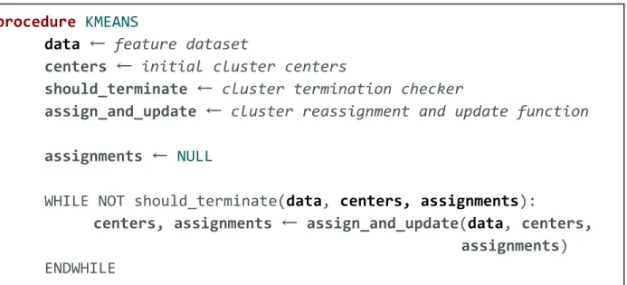
pseudocode for our clustering algorithm in Figure 1. This algorithm is almost identical to the description of k-means in Section 2.3, except that we have abstracted the termination condition from being “the cluster centers are unchanged” to a generic function that checks before each iteration of clustering whether we should terminate clustering at the current iteration. This function could be implemented according to any of the options discussed in Section 2.6. In addition, we have combined the cluster assignment and cluster center update steps into one function.
The reason for this abstraction is that for methods like mini-batch k-means that do not update the assignments for all of the points simultaneously, this abstraction allows us to present a uniform interface from the point of view of the k-means procedure, regardless of whether we are implementing that an algorithm like mini-batch k-means or not. It should be noted that the similarity metric as discussed in Section 2.4 will be used in this function, since it is needed to determine cluster assignments.
procedure KMEANS
data ← feature dataset
centers ← initial cluster centers
should_terminate ← cluster termination checker
assign_and_update ← cluster reassignment and update function
assignments ← NULL
WHILE NOT should_terminate(data, centers, assignments):
centers, assignments ← assign_and_update(data, centers,
assignments)
ENDWHILE
Figure 1: Clustering Algorithm Pseudocode
To implement the algorithm, we chose to use the Python programming language. We chose Python because it is a well-known programming language, and it has very flexible data types. It is this flexibility that will allow us to pass in different types of termination condition checkers (e.g. functions or classes that act like functions). Furthermore, Python has the powerful numpy library, which allows us to use matrix and vector operations very efficiently to compute cluster assignments and update cluster centers. Using this vectorization, we can define the similarity metric on a per-feature basis, meaning that when numpy tries to compute the similarity metric between a feature vector and a cluster mean vector, the appropriate similarity metric will
be called automatically for each element in these vectors. This is why we do not have to pass in a similarity metric function into our pseudocode from Figure 1. In some regard, the similarity metric is engendered into the dataset that we pass in. However, we just need a library that accesses it, and numpy handles this task perfectly. Finally, Python has numerous other statistical and data science packages like pandas, matplotlib, statsmodels, and scikit-learn that are
extremely useful for visualizing the data and providing a transparent view into the clustering and the final results (e.g. pandas, matplotlib). We can also use these libraries (in particular, scipy and statsmodels) for executing the significance tests discussed in Section 2.5, which is important if we want to experiment with many of the cluster quality and termination measurements
described in Sections 2.5 and 2.6.
3. Experiments
3.1. Experimental Dataset
For this paper, we ran and tested the algorithm over a fabricated dataset that is meant to be representative of the type of data that might actually be used at a real bank. The data contains 100,000 rows and was stored in a CSV file for our use. Each row contains information regarding a customer. It should be noted that for the purposes of this dataset, the customer as discussed in the previous sections will be referred to as a household, which is a collection of individual people or businesses. Thus, we will be clustering together households instead of individual people. In this context, households are not necessarily familial. They can also refer to businesses, which can of course be comprised of multiple people, such as business partners. Sometimes, they are comprised of people and businesses. This establishment of semantics is
necessary in order to understand the features that are provided for each household. Each household has 28 different features, which are broken down as follows:
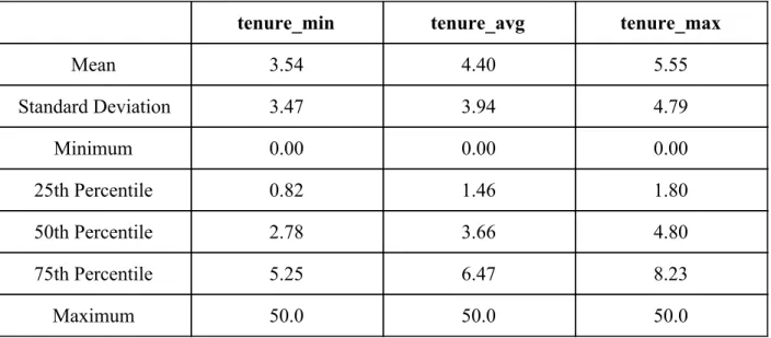
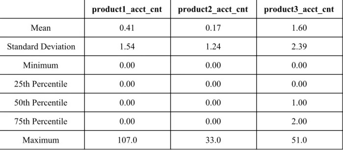
1) Client Tenure (3 features)
Client tenure refers to how long an individual (or business) has been engaging with services at the bank, measured in years, with fractions of a year allowed. Each household
contains three summary statistics for client tenure of its members: tenure_min (minimum tenure), tenure_max (maximum tenure), and tenure_avg (average tenure). These columns were checked and cleaned to ensure that their values fell in a reasonable range, which was between 0 and 50. Their summary statistics are presented in Table 1 below:
tenure_min tenure_avg tenure_max
Mean 3.54 4.40 5.55 Standard Deviation 3.47 3.94 4.79 Minimum 0.00 0.00 0.00 25th Percentile 0.82 1.46 1.80 50th Percentile 2.78 3.66 4.80 75th Percentile 5.25 6.47 8.23 Maximum 50.0 50.0 50.0
Table 1: Client Tenure Summary Statistics 2) Transaction Data (8 features)
This data refers to the money that has been transferred into and out of household
accounts. The first two features are transaction_cnt and transaction_net, which refer to the total number of transactions and net money (in dollars) transferred into the household’s accounts.
Transactions can be differentiated by where they were initiated, so we have two more features tran_with_Bank_cnt and tran_with_Bank_net to represent analogous figures but over just the transactions initiated at this bank. Transactions are broken down into two types: type1 and type2. For each type, we have the total number of transactions (tran_type1_cnt and tran_type2_cnt) and the total balance of the accounts involved in transactions of each type (tran_type1_bal and tran_type2_bal). Their summary statistics are presented in Tables 2 and 3 below:
transaction_ cnt transaction_ net ($) tran_with_Bank_ cnt tran_with_Bank_ net ($) Mean 424.6 1.30 * 105 305.6 1.54 * 105 Standard Deviation 647.1 1.09 * 106 439.9 1.10 * 106 Minimum 0.00 −3.27 * 107 0.00 −3.23 * 107 25th Percentile 0.00 −1.20 * 105 0.00 −1.06 * 105 50th Percentile 147.5 0.00 140.0 0.00 75th Percentile 650.0 2.93 * 105 470.0 3.24 * 105 Maximum 11795.0 5.64 * 107 7782.0 5.61 * 107 Tables 2 and 3: Overall Transaction Counts and Net Transfers (top), Overall Transaction Counts and Balances (bot.)
tran_type1_cnt tran_type1_bal ($) tran_type2_cnt tran_type2_bal ($) Mean 166.8 3.05 * 105 261.5 −1.75 * 105 Standard Deviation 275.8 3.05 * 106 373.0 2.02 * 106 Minimum 0.00 −8.89 * 107 0.00 −9.93 * 107 25th Percentile 0.00 −3.70 * 105 0.00 −4.83 * 105 50th Percentile 17.0 0.00 129.0 0.00 75th Percentile 253.0 7.48 * 105 398.0 2.80 * 105 Maximum 5043.0 1.56 * 107 6757.0 5.61 * 107