On fixed-point hardware polynomials

HAL Id: hal-01214739

https://hal.inria.fr/hal-01214739

Preprint submitted on 12 Oct 2015

HAL is a multi-disciplinary open access

archive for the deposit and dissemination of

sci-entific research documents, whether they are

pub-lished or not. The documents may come from

teaching and research institutions in France or

abroad, or from public or private research centers.

L’archive ouverte pluridisciplinaire HAL, est

destinée au dépôt et à la diffusion de documents

scientifiques de niveau recherche, publiés ou non,

émanant des établissements d’enseignement et de

recherche français ou étrangers, des laboratoires

publics ou privés.

On fixed-point hardware polynomials

Florent de Dinechin

To cite this version:

On fixed-point hardware polynomials

Florent de Dinechin

Univ Lyon, INSA, CITI Lab

[email protected]

F

Abstract—Polynomial approximation is a general technique for the eval-uation of numerical functions of one variable. This article addresses the automatic construction of fixed-point hardware polynomial evaluators. By systematically trying to balance the accuracy of all the steps that lead to an architecture, it simplifies and improves the previous body of work covering polynomial approximation, polynomial evaluation, and range reduction. This work is supported by an open-source implementation.

Index Terms—elementary function; hardware evaluator; polynomial ap-proximation; computer arithmetic;

1

I

This article addresses the automatic construction of fixed-point polynomial evaluators for a real function f of one real variable x over a closed interval I. This is a very generally useful building block when designing hardware functions in fixed-point [1], [2], [3] or floating-point [4], [5], [6] for application-specific processors or reconfigurable computing [7], [8]. This article refines several previous works describing generic function approximators [9], [10], [11]: tools that input a function and parameters specifying its context, and produce an architecture, as illustrated by Figure 1.

The construction of a polynomial evaluator typically proceeds in three steps. The first is the computation if a polynomial that approximates the function f . The second is the generation of adders and multipliers that will evaluate this polynomial. These two steps are usually preceded by a range-reduction that transform the initial function into one more suited for polynomial approximation [12], [10], [6].

The main constribution of this article is to show that these three steps (Sections 2 to 4) are deeply linked by arithmetic considerations. Expliciting these links enables a very simple derivation of near-optimal values of most architectural parameters, for which previous works often

Functional spec. Performance spec.

architecture generator function f : [0, 1) →?

input precision `in

output format (mout, `out)

degree FPGA frequency vhdl

Fig. 1. Interface to a generic fixed-point function approximator

×

_×

_×

a0

a1

a2

a3

Polynomial Coefficient Table

xin i address α w x w − α f x3 fx2 f x3= x e p(x) final round _y

Fig. 2. A polynomial evaluator (uniform segmentation, Horner scheme)

resort to complex heuristics. Several minor improvements are introduced on the way.

This work is supported by an open-source implementation in the FloPoCo1 _{generator [13].}

Approximation and evaluation are implemented as the BasicPolyApprox and FixHornerEvaluator classes, while the FixFunctionBySimplePoly and FixFunctionByPiecewisePolyclasses combine them to build architectures. The interested reader will find in their respective source code all the details not exposed here for clarity.

1.1 Unit intervals

We assume that f is continuously differentiable over a closed interval I up to a certain order. In this work, we will systematically normalize I to [0, 1] or [−1, 1]. Any function g that has a different input interval may be transformed into a function f on I = [0, 1] or I = [−1, 1] by means of a suitable change of variable. Technically, in all practical cases, there exists an affine transformation g such that g([−1, 1]) = I and g entails little or no additional hardware cost. We then consider f ◦ g(x) on [−1, 1]. Examples will be given in the sequel.

The reason for normalizing functions to unit intervals is that it greatly simplifies the arithmetic analysis needed to build an efficient architecture. This is indeed at the core of the contributions of this article. In other words, if a function has, in its original context, a different input range (for instance [0, 2−k] after range reduction in [2] or [4]), the present work claims that rewriting it as a function on [0, 1] or [−1, 1] is relevant for a fixed-point implementation.

1.2 Fixed-point formats

Following the VHDL standard, a fixed-point format is de-fined by two integers (m, `) that respectively denote the position of the most significant and least significant bit (MSB and LSB) of the data. The respective values of the MSB and LSB are thus 2m and 2`. The LSB position ` denotes the precision of the format. The MSB position denotes its range. Both m or ` can be negative if the format includes fractional bits. In signed arithmetic, m is the position of the sign bit.

For instance, on Figure 1, an input in [0, 1] is represented in the (−1, `in) format.

1.3 Error analysis for computing just right

One key idea of this work is that architectures should

com-pute, at each step, accurately enough, but no more, if more accuracy costs hardware or latency. Formally, accuracy is achieved by bounding errors. An error, denoted ε, is always defined as the difference between two values, one being more accurate than the other. For instance, εtotal= y − f (x)

is the error of the computed output y with respect to the real value of the function f (x). This error should not exceed the value of the LSB of the output: ∀x ∈ I, |εtotal| < 2`out.

In-deed, a higher accuracy cannot be expressed on the output, while a lower accuracy would mean that some outputs bits hold no useful information. Therefore, the output precision `_outalso serves to specify the accuracy of the implementation (Figure 1). This accuracy objective is often termed faithful rounding in the literature.

The maximal absolute value of an error ε over the interval I is noted ε, so the previous objective can also be stated as εtotal< 2`out.

This total error is decomposed as follows. The function f is approximated by a polynomial p, with error εapprox(x) =

p(x)−f (x). The evaluation of p(x) involves rounding errors: the value actually computed by the hardware will be noted e

p(x). The sum of all rounding errors in the architecture is noted εeval(x) =p(x) − p(x). Ase p(x) must be evaluated toe an internal precision slightly higher than `out, it finally needs

to be rounded to the target format: εfinal round = y −p(x) ise the corresponding error. Thus,

εtotal = y − f (x)

= y −p(x) +_e p(x) − p(x) + p(x) − f (x)_e = εfinal round+ εeval+ εapprox (1)

Here, εfinal roundis actually the dominant source of error.

It is, at worst, one half of the weight of the output LSB: ε_{final round} = 2`out−1<sub>. The constraint on the two other errors</sub> to ensure εtotal< 2`outis therefore εapprox+ εeval< 2`out−1.

To balance the errors, the polynomial approximation step is given the error budget εtargetappprox = 2`out−2. The

approxima-tion step computes the polynomial of minimum degree that allows to match this error budget. It also reports the actual ε_approx. This defines the error budget for the evaluation as εtarget_eval = ε_{final round} − εapprox. This value is passed to

the generator of polynomial hardware, whose task is to dimension the adders and multipliers to achieve it. This process is illustrated on Figure 3.

FixFunctionBySimplePoly

BasicPolyApprox FixHornerEvaluator

.vhdl

f,`in,`out

f, εtargetappprox d, p, εapprox p, εtargeteval arch. param.

Fig. 3. Execution flow of a basic polynomial approximator

1.4 Generic range reduction techniques

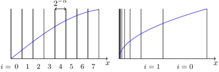
This general error analysis scheme may be adapted to most range reduction techniques. For example, the architecture of Figure 2 implements the uniform segmentation scheme [9], [11]: it splits the input interval into 2α _{sub-intervals of}

identical size (Figure 5, left). An approximation polynomial can then be used on each interval. The coefficients are stored in a table addressed by the α MSBs of the input (noted i throughout this paper). The motivation for this is that the same accuracy can be obtained with polynomials of smaller degree on the smaller intervals. Actually, in such a scheme, the degree is an input to the generator. The generator computes the smallest α that entails that the target accuracy can be reached with this degree (see Figure 4). Thus, the degree is a way of controlling the trade-off between table cost and arithmetic cost.

FixFunctionByPiecewisePoly PiecewisePolyApprox BasicPolyApprox FixHornerEvaluator FixMultAdd .vhdl f,`in,`out,d

f, εtargetappprox, d α, {pi}, εapprox fi, ε target appprox pi, εapprox,i {pi}, ε target eval {(mj, `j)}

Fig. 4. Execution flow of FixFunctionByPiecewisePoly

In such a scheme, the previous error analysis simply needs to consider the worst case over the sub-intervals i: the error approximation target must be reached by all the approximation polynomials pi, each on its sub-interval; the

evaluation error budget is computed out of the worst-case error over i; finally, the evaluation hardware needs to be shared among all the intervals, so its datapath must be dimensioned to fit all i. This simply consists in considering, for each fixed-point format, the max (over i) of the MSBs and the min of the LSBs.

Some functions have singularities on the interval end-points (for instance the square root depicted on Figure 5, right). They may be best implemented by power-of-two segmentation [10]. The only difference with uniform

seg-x i = 0 1 2 3 4 5 6 7 2−α x i = 0 i = 1

mentation is that the interval index is obtained by a leading-zero or leading-one counter, while the reduced argument is obtained by the corresponding shift on the input. These leading zero counters and shifters must be added to Fig-ure 2.

Hierarchical segmentation is studied in [10]. The conclu-sion is that two levels always suffice in practice, with only the outer one needing power-of-two splitting.

This paper is demonstrated on the simpler uniform segmentation scheme, but the techniques presented here (in particular in Section 3) apply to all these other generic range reduction techniques, and even to function-specific range reductions [12], [2], [3], [4], [6].

2

P

Textbooks [12] provide many methods for approximating a function with a polynomial. Taylor or Chebyshev are well-known analytical methods, but the best approximations are provided by Remez’ algorithm, a numerical process that, under some conditions, converges to the minimax approx-imation: the polynomial premez of degree d that minimizes

||p − f ||∞. A problem is that the coefficients of premezare real

numbers that must be rounded to finite-precision machine numbers. This introduces a new error that has to be taken into account [9], [10]. Besides, this gives a new polynomial e

p_remezwhich is in general no longer the best possible among the polynomials whose coefficients are machine numbers.

The state of the art is therefore the modified Remez algorithm [14] available as the fpminimax command of the Sollya tool [15]. It directly provides a minimax polynomial among the polynomials whose coefficients satisfy some user-specified constraints. These constraints specify the LSB weight of each coefficient.

To define these constraints, consider a theoretical ar-chitecture evaluating the developed form of a polynomial a0+ a1x + a2x2+ . . . + adxd on I = [0, 1] or I = [−1, 1].

It would first compute each monomial ajxj, then align

them to compute the fixed-point sum. Such an alignment is depicted on Figure 6 for a polynomial evaluating f (x) = ex on [0, 1] to an accuracy of 10−6 (it is close to the Taylor series).

As |x| ≤ 1 we also have |xj_{| ≤ 1, hence |a}

jxj| ≤ |aj|.

Therefore the MSB of each monomial term ajxjis that of aj.

Let us now discuss the LSBs to derive the constraints to input to fpminimax. There is no point in evaluating one of the monomials much more accurately than the others, as the sum will be no more accurate than its least accurate term. Besides, for x close to 1, the monomial ajxjcannot be

more accurate than ajitself. A near-optimal design decision

is therefore to have each ajaccurate to the same LSB `a. The

maximal value of `amay be determined out of the accuracy

`a a0 1.000000000000 a1 0.111111111100 a2 0.100000100101 a3 0.001001000010 a4 0.000100011011 a0 1.000000000000 +a1x 0.xxxxxxxxxxxx... +a2x2 0.xxxxxxxxxxxx... +a3x3 0.00xxxxxxxxxx... +a4x4 0.000xxxxxxxxx... = s.ssssssssssss... Fig. 6. Ifx ∈ [−1, 1], the alignment of theajxjfollows that of theaj

objective εtargetappprox. Intuitively, we need 2`a ≤ εtargetappprox so

the coefficients hold information that is at least as accu-rate as εtargetappprox. In practice, surprisingly, there usually exist

polynomials satisfying εapprox ≤ ε target

appprox even when 2`a is

sligthly larger than εtargetappprox. This effect improves with the

degree d, therefore a good heuristic is to start by calling fpminimaxwith `a = dlog2(ε

target

appprox × d)e. If fpminimax

fails to obtain a polynomial that satisfies εapprox < εtargetappprox,

then `ais decreased until it succeeds. This loop (formalized

in Algorithm 1) rarely needs more than a few attempts and its execution time remains well below one second. It is implemented in FloPoCo in the BasicPolyApprox class. The computation of εapprox is performed with Sollya

supnorm(p, f, I) command [16].

Algorithm 1Approximation for I = [0, 1] or I = [−1, 1]

1: procedureFIXEDPOINTPOLYAPPROX(f, d, I, εtargetappprox)

2: `a← dlog2(ε target appprox× d)e − 1 3: repeat 4: `a ← `a+ 1 5: p ← fpminimax(f, d, I, {`a}) 6: εapprox← supnorm(p, f, I)

7: until εapprox ≤ εtargetappprox

8: end procedure

This reasoning assumed a theoretical architecture eval-uating the developed form, but it actually holds for any evaluation scheme. For instance, let us consider the classical Horner evaluation scheme, used in most previous work [9], [10], [11] because it minimizes the number of operations :

p(x) = a0+ x × (a1+ x × (a2+ .... + x × ad)...) . (2)

It can be expanded in the following recurrence:        σd= ad πj= x × σj+1 ∀j ∈ {0 . . . d − 1} σj= aj+ πj ∀j ∈ {0 . . . d − 1} p(x) = σ0 (3)

The reader may observe that, for |x| ≤ 1, having all the aj accurate to the same LSB `a again entails a recurrence

where no step is needlessly more accurate than the others: Algorithm 1 also works in this case. The same will be true of evaluation schemes intermediate between Horner and the developed form, such as Estrin’s [12].

3

A

The analysis of the previous section is based on the fact that the function input range is normalized to [0,1] or [-1,1]. But the purpose of argument range reduction is, as the name suggest, to reduce this interval. For instance, the architecture of Figure 2 actually evaluates f (xin) on small sub-intervals,

e.g. xin∈ [0, 2−α], enabling smaller-degree polynomial than

on the full interval.

Let us define the change of variable xin = 2−αx, such

that f (xin) = f (2−αx) = g(x) for x ∈ [0, 1]. Note that

it translates both the MSB and the LSB of xin by α

posi-tions. Applied to an approximation polynomial, this change of variables gives pf(xin) = a0 + a1xin + a2xin2. . . =

reduction can also be viewed as a reduction of the polyno-mial coefficients, here by a factor 2jα _{for the coefficient of}

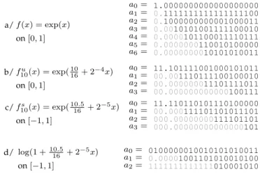
degree j. This is illustrated by Figure 7 on a few examples extracted from uniform piecewise approximations to exp and log. Having normalized the function to a unit interval then enables the use of Algorithm 1.

As a parenthesis, Figure 7 also gives a visual clue how the degree is determined by the target accuracy. Indeed, on Figures 7b/ and 7c/, a 4-th degree coefficient a4 would

be to the right of the picture, contributing no useful bits. However, this is only true if all the coefficients have the same sign, as Figure 7d/ illustrates. In the general case, the Sollya command guessdegree(f, I, εtargetappprox) provides

a good estimate of the degree needed to reach a given accuracy.

In [9], [10], or [11], the change of variable used is xin = 2−α(i + x) for x ∈ [0, 1) and i ∈ {0, 1 . . . 2α− 1}.

The normalised i-th function is fu

i (x) = f (2−α(i + x)). The

reduced argument x is obtained as the LSBs of xin in the

case of uniform segmentation (Figure 2), as a shift of xinin

the case of power-of-two segmentation.

One novelty of the present work is to center x on its sub-interval: we introduce the change of variable xin =

2−α(i+1₂+x₂0) for x0 ∈ [−1, 1). The normalised i-th function becomes fis(x0) = f (2−α(i +

1 2+

x0

2)). In general, this leads

to smaller coefficients for the approximation polynomials, as illustrated by Figure 7c/ versus 7b/. The architectural overhead to obtain x0out of x is limited to one inverter (not shown on Figure 2 for simplicity) to complement the MSB of x. Its delay is largely hidden by the table access delay.

Another remark can be made about the sign of the coef-ficients: analytical properties of the function (monotinicity, convexity, and so on) are defined by the signs of the succes-sive derivatives. Good approximation polynomials typically inherit these properties, which are then often reflected in the signs of the corresponding coefficients. For instance, on Figure 7, all the coefficients for the various exponentials are positive. As a consequence, for a piecewise approximation of an elementary function, it is typical (but not automatic due to numerical artifacts) that all the coefficients of a given degree have the same sign. In this case, the sign bit need not be stored, saving one bit per coefficient.

4

P

This section discusses the sizing of all variables on the Horner evaluator of Figure 2. As for evaluation, it can be straightforwardly extended to other schemes. .

Consider one Horner step of (3). As the ajare known, it

is possible to compute the ranges of the πj and eσj, hence their MSBs, by straightforward interval evaluation of (3) on [−1, 1]. This is implemented in a procedure COMPUTE-HORNERMSBS. In the typical scenario where x is a reduced argument, aj is larger in magnitude than πj, therefore the

MSB of σjwill be that of aj, sometimes plus one (overflow

bit to the left). This is the case depicted on Figure 8. How-ever it may also happen that ajis smaller in magnitude than

πj.

Concerning the LSBs, we have two opportunities of reducing the size of intermediate computations. Firstly, the product πj may be rounded or truncated at each step,

a/f (x) = exp(x) on[0, 1] a0= 1.0000000000000000000 a1= 0.1111111111111111100 a2= 0.1000000000001000011 a3= 0.0010101001111100010 a4= 0.0000101100011110111 a5= 0.0000000110010100000 a6= 0.0000000010101010011 b/fu 10(x) = exp( 10 16+ 2 −4_x) on[0, 1] a0= 11.101111001000101011 a1= 00.001110111100100010 a2= 00.000000011101111011 a3= 00.000000000000100111 c/fs 10(x) = exp( 10.5 16 + 2 −5_x) on[−1, 1] a0= 11.110110101110100000 a1= 00.000111101101011101 a2= 000.00000000111101101 a3= 000.00000000000000101 d/ log(1 +10.5₁₆ + 2−5x) on[−1, 1] a0= 0100000010010101010011 a1= 0.00001001101010010100 a2= 1111111111111010001010 Fig. 7. Range reduction reduces theaj. All the polynomials are accurate to10−6;f10u andf10s cover the same sub-interval ofexp(x).

entailing an error bounded by επ(j). Secondly, x may also

be truncated to reduce the multiplier size (informally, to remove bits of x that the multiplication by σj+1 will shift

so far right that they don’t affect the result – the formal for-mulation follows). This truncation of x was a contribution of [11].

The recurrence that is actually computed is thus:        e σd= ad e πj=xej×σej+1+ επ(j) ∀j ∈ {0 . . . d − 1} e σj= aj+eπj ∀j ∈ {0 . . . d − 1} e p(x) = σ0

Remark that the addition is exact, since it is a fixed-point addition.

The evaluation error of step j can now be defined as: εeval(j) =σej− σj= (aj+πej) − (aj+ πj) =πej− πj

=πej−xejσej+1 + xejσej+1− xjσj+1

= επ(j) +xejeσj+1− xjσej+1 + xjσej+1− xjσj+1 = επ(j) + (xej− xj)eσj+1 + xjεeval(j + 1) .

(4) Algorithm 2 computes all the MSBs and LSBs of the Horner datapath of Figure 2 according to (4). It is a loop again: it computes εeval = εeval(0), and adds more LSB bits

if this error exceeds the target. Again, the argument that no step needs to be more accurate than the others drives us to have a common LSB `σ. It will be the LSB of all the σj but

also of the πj (see Figure 8). As σj = aj+πej, σj must be at least as accurate as aj, otherwise bits of ajwould be useless.

Therefore, line 3 of Algorithm 2 initializes `σto `a.

Let us now address the truncation of x. If exj has the LSB `x,j, we have |exj − xj| < 2`x,j, and the term (exj −

xj)eσj+1can be bounded as |σej+1(exj− xj)| ≤ 2

mσ,j+1_{· 2}`x,j where mσ,j+1is the MSB ofeσj+1. Balancing this error term and επ(j) yields 2mσ,j+1· 2`x,j = 2`σ. This defines `x,j =

`a `σ

aj aaaaaaaaaaaa 1

+πj pppppppppppppppppppp

= σj ssssssssssssssss

rounding bit

`σ− mσ,j+1. In practice, it is a truncation only if `x,j < `x.

Otherwise, x is not truncated and this first error term is zero. In the typical case where the MSB of aj(hence σj) grows as

j decreases (Figure 6), truncation of x happens in the earlier Horner steps.

A word now on the truncation of the product. If the hard-ware (for instance a fixed-size FPGA DSP block) computes the full productxejeσj+1, rounding it toπejis almost for free: it can be achieved by extending the addition aj +eπj one bit on the right to add a constant bit before truncation to `σ (Figure 8). In this case επ = 2`σ−1. Otherwise, a cheaper

alternative is to use an ad-hoc FixMultAdd operator which combines a faithful truncated multplier and an adder in a single compression tree. In this case επ= 2`σ.

Algorithm 2Determining Horner evaluator parameters

1: procedureHORNERSIZING(`x, {ma,j}, `a, εtarget_eval )

2: {mσ,j} = COMPUTEHORNERMSBS() 3: `σ← `a 4: repeat 5: εeval= 0 6: for i = d − 1 down to 0 do 7: `x,j ← max(`x, `σ− mσ,j+1) 8: if `x,j 6= `xthen . if x truncated

9: ε_eval= ε_eval+ εx . add its error

10: end if

11: εeval= εeval+ επ . πjalways truncated

12: end for

13: if εeval > εtargeteval then . not accurate enough:

14: `σ← `σ− 1 . need more LSB bits

15: end if

16: until εeval ≤ εtargeteval

17: end procedure

5

R

The techniques described in this article lead to consistently improved architectures with respect to those previously published. Table 1 shows typical improvements of coeffi-cient sizes and multiplier sizes with respect to the previous state of the art: FloPoCo 2.3.1, which was used to write [11].

TABLE 1

The proposed method leads to smaller data paths.

Version Table Multipliers

f (x) = 0.5√1 + x,`in= `out= −23,d = 2 2.3.1 256×(27+19+10) 16×20, 16×10 Present 64×(26+17+9) 17×18, 10×10 f (x) = 0.5√1 + x,`in= `out= −52,d = 4 2.3.1 256×(56+46+36+28+19) 44×49, 35×37, 25×29, 25×19 Present 256×(56+44+33+23+14) 44×47, 36×36, 26×26, 15×15 f (x) = log(1 + x),`in= `out= −23,d = 2 2.3.1 256×(27+21+13) 16×22, 16×13 Present 128×(26+18+9) 16×20, 10×10 f (x) = log(1 + x),`in= `out= −52,d = 4 2.3.1 512×(56+49+40+32+23) 44×50, 44×41, 35×33, 25×23 Present 512×(56+46+35+24+14) 43×48, 37×37, 26×26, 15×15 All the architectures reported there were tested for last-bit accuracy thanks to the FloPoCo test framework [13].

However the main contribution of this work is a much simpler view of the problem, thanks to normalization to unit intervals and systematic balancing of errors. This lead to much cleaner and more robust open-source code.

This is a solid foundation on which to explore other range reductions [10], other evaluation schemes [12], [17], and FPGA-specific optimizations based on fixed-size mem-ory and DSP blocks. Also, we have used the phrase “near optimal” in the introduction: it is usually still possible to shave one more bit here and there by relaxing the constraint that all the degrees share the same LSB. Is it worth the increased code complexity?

Acknowledgmentsto the Sollya team (N. Brisebarre, S. Chevillard, M. Joldes, Ch. Lauter), and to D. Thomas and J.M. Muller for discussions on this subject. This work was supported by the ANR INS MetaLibm project.

R

[1] R. Cheung, D.-U. Lee, W. Luk, and J. Villasenor, “Hardware gen-eration of arbitrary random number distributions from uniform distributions via the inversion method,” IEEE Transactions on VLSI Systems, vol. 8, no. 15, 2007.

[2] F. de Dinechin, M. Istoan, and G. Sergent, “Fixed-point trigono-metric functions on FPGAs,” SIGARCH Computer Architecture News, vol. 41, no. 5, pp. 83–88, 2013.

[3] F. de Dinechin and M. Istoan, “Hardware implementations of fixed-point Atan2,” in 22nd Symposium of Computer Arithmetic. IEEE, Jun. 2015.

[4] F. de Dinechin and B. Pasca, “Floating-point exponential functions for DSP-enabled FPGAs,” in Field Programmable Technologies, Dec. 2010, pp. 110–117.

[5] F. de Dinechin, P. Echeverr´ıa, M. L ´opez-Vallejo, and B. Pasca, “Floating-point exponentiation units for reconfigurable comput-ing,” Transactions on Reconfigurable Technology and Systems, vol. 6, no. 1, 2013.

[6] D. B. Thomas, “A general-purpose method for faithfully rounded floating-point function approximation in FPGAs,” in 22d Sympo-sium on Computer Arithmetic. IEEE, 2015.

[7] N. Kapre and A. DeHon, “Accelerating SPICE model-evaluation using FPGAs,” Field-Programmable Custom Computing Machines, pp. 37–44, 2009.

[8] F. de Dinechin and B. Pasca, High-Performance Computing using FPGAs. Springer, 2013, ch. Reconfigurable Arithmetic for High Performance Computing, pp. 631–664.

[9] D. Lee, A. Gaffar, O. Mencer, and W. Luk, “Optimizing hardware function evaluation,” IEEE Transactions on Computers, vol. 54, no. 12, pp. 1520–1531, 2005.

[10] D.-U. Lee, P. Cheung, W. Luk, and J. Villasenor, “Hierarchical segmentation schemes for function evaluation,” IEEE Transactions on VLSI Systems, vol. 17, no. 1, 2009.

[11] F. de Dinechin, M. Joldes, and B. Pasca, “Automatic generation of polynomial-based hardware architectures for function evalu-ation,” in Application-specific Systems, Architectures and Processors. IEEE, 2010.

[12] J.-M. Muller, Elementary Functions, Algorithms and Implementation, 2nd ed. Birkh¨auser, 2006.

[13] F. de Dinechin and B. Pasca, “Designing custom arithmetic data paths with FloPoCo,” IEEE Design & Test of Computers, vol. 28, no. 4, pp. 18–27, Jul. 2011.

[14] N. Brisebarre and S. Chevillard, “Efficient polynomialL∞- ap-proximations,” in 18th Symposium on Computer Arithmetic. IEEE, 2007, pp. 169–176.

[15] S. Chevillard, M. Joldes¸, and C. Lauter, “Sollya: An environment for the development of numerical codes,” in Int. Conf. on Mathe-matical Software, ser. LNCS, vol. 6327. Springer, 2010, pp. 28–31. [16] S. Chevillard, M. Joldes, and C. Lauter, “Certified and fast

com-putation of supremum norms of approximation errors,” in 19th Symposium on Computer Arithmetic. IEEE, 2009, pp. 169–176. [17] J. Detrey and F. de Dinechin, “Table-based polynomials for fast

hardware function evaluation,” in Application-specific Systems, Ar-chitectures and Processors. IEEE, 2005, pp. 328–333.