Hollow cathode modeling: I. A coupled plasma thermal two-dimensional model

HAL Id: hal-02326760

https://hal.archives-ouvertes.fr/hal-02326760

HAL is a multi-disciplinary open access archive for the deposit and dissemination of sci-entific research documents, whether they are pub-lished or not. The documents may come from teaching and research institutions in France or abroad, or from public or private research centers.

L’archive ouverte pluridisciplinaire HAL, est destinée au dépôt et à la diffusion de documents scientifiques de niveau recherche, publiés ou non, émanant des établissements d’enseignement et de recherche français ou étrangers, des laboratoires publics ou privés.

Gaétan Sary, Laurent Garrigues, Jean-Pierre Boeuf

To cite this version:

Gaétan Sary, Laurent Garrigues, Jean-Pierre Boeuf. Hollow cathode modeling: I. A coupled plasma thermal two-dimensional model. Plasma Sources Science and Technology, IOP Publishing, 2017, 26 (5), pp.055007. �10.1088/1361-6595/aa6217�. �hal-02326760�

H

OLLOW CATHODE MODELING

:

I.

A COUPLED PLASMA

-THERMAL TWO

-

DIMENSIONAL MODEL

Gaétan Sary1,2_{, Laurent Garrigues}1,2_{, and Jean-Pierre Boeuf}1,2

1_{Université de Toulouse ; UPS, INPT ; LAPLACE (Laboratoire Plasma et Conversion d’Energie) ; 118 route de}

Narbonne, F-31062 Toulouse cedex 9, France.

2 _{CNRS ; LAPLACE ; F-31062 Toulouse, France.}

E-mail: sary@laplace.univ-tlse.fr

A

BSTRACT

A two dimensional axisymmetric quasi-neutral fluid model of an emissive hollow cathode that includes neutral xenon, single charge ions and electrons has been developed. The gas discharge is coupled with a thermal model of the cathode into a self-consistent generic model applicable to any hollow cathode design. An exhaustive description of the model assumptions and governing equations is given. Boundary conditions for both the gas discharge and thermal model are clearly specified as well. A new emissive sheath model that is valid for any emissive material and in both space charge and thermionic emission limited regimes is introduced. Then, setting the emitter temperature to an experimentally measured profile, we compare simulation results of the plasma model to measurements available in the literature for NASA NSTAR barium oxide cathode. Qualitative discrepancies between simulation results and measurements are noted in the cathode plume regarding the simulated plasma potential. Motivated by experimental evidence supporting the occurrence of ion acoustic instabilities in the cathode plume, an enhanced model of electron transport in the plume is presented and its consequences analyzed. Using the obtained plasma model, simulated quantities in the plume are qualitatively comparable with measurements. Inside the cathode, the simulated plasma density agrees well with measurements and is within the ±50 % experimental uncertainty associated with these measurements.

A comparison of simulation results of the full coupled cathode model for the NASA NSTAR cathode with experimental measurements is presented in a companion paper, as well as a physical analysis of the cathode behavior and a parametric study of the influence of the operating point and key design choices.

3 4 5 6 7 8 9 10 11 12 13 14 15 16 17 18 19 20 21 22 23 24 25 26 27 28 29 30 31 32 33 34 35 36 37 38 39 40 41 42 43 44 45 46 47 48 49 50 51 52 53 54 55 56 57 58 59 60

N

OMENCLATURE

= deviatoric viscous stress tensor for neutral species = dynamic viscosity of neutral xenon

= plasma potential

= plasma production source term

= momentum exchange term for species s due to elastic collisions with other species = energy exchange term for species s due to elastic collisions with other species = plasma potential

= 1st _{ionization energy of Xe atoms.}

, = elastic collision rate between species and , = collision frequency of species with species

= thermal conductivity of species s = current density of species s

Γ = particle flux of species s at a boundary of the fluid domain = discharge current

= electron mobility = xenon mass flow rate = work function

= effective work function or potential barrier that opposes thermionic emission = local emitter temperature

3 4 5 6 7 8 9 10 11 12 13 14 15 16 17 18 19 20 21 22 23 24 25 26 27 28 29 30 31 32 33 34 35 36 37 38 39 40 41 42 43 44 45 46 47 48 49 50 51 52 53 54 55 56 57 58 59 60

= standard cubic centimeter 3 4 5 6 7 8 9 10 11 12 13 14 15 16 17 18 19 20 21 22 23 24 25 26 27 28 29 30 31 32 33 34 35 36 37 38 39 40 41 42 43 44 45 46 47 48 49 50 51 52 53 54 55 56 57 58 59 60

I

NTRODUCTION

Hollow cathodes are critical components of Hall Thrusters (HTs). Since they provide electrons for both the discharge chamber and beam neutralization, the resulting current draw may be quite important and as large as 100 A. With the advent of higher power HTs comes an increasing demand for cathodes capable of supplying large discharge currents. With this goal in mind, it is crucial to study the physics of hollow cathodes, so as to understand the important mechanisms playing a role in the cathode, and in turn to determine scaling laws which might aid the development of new more powerful, more efficient, and more durable cathodes. A typical hollow cathode geometry is represented in fig. 1.

Hollow cathodes have been studied extensively both theoretically [1–9] and experimentally [10–14]. Many aspects relevant to the cathode operation have been the topic of specific modeling studies such as the numerical modeling of the interior plasma region [1] and of the near plume plasma [3,5] or the description of electron emission physics and the influence of emitter surface features [8]. Thanks to this wide literature, hollow cathodes using barium oxide (BaO) as an electron emitter are well understood and the region inside the cathode has been numerically modelled with a very high degree of accuracy[8]. An extensive account of an existing numerical model (Orca2D) developed by Mikellides et al. at the Jet Propulsion Laboratory is given in [5] and references therein. Yet, most of these contributions to hollow cathode modeling focus on a single operating point for one cathode design. Only little work has been done to globally describe the influence of design choices and of the operating conditions on the discharge[15,16].

Figure 1: Typical hollow cathode geometry. A support tube holds an emissive insert which is self-heated by plasma bombardment. The heater provides initial heating of the emitter. The keeper is not represented.

In this work, we will present a numerical model of both the interior region and the near plume of a hollow cathode. Similarly to existing fluid models (e.g. [3,8,9]), the model presented here is a 2D-axisymmetrical quasi-neutral model which treats quasi-neutrals, ions and electrons as separate fluids. Plasma sheath and most importantly emissive sheaths are accounted for through a new first principles based emissive sheath model which is valid in 3 4 5 6 7 8 9 10 11 12 13 14 15 16 17 18 19 20 21 22 23 24 25 26 27 28 29 30 31 32 33 34 35 36 37 38 39 40 41 42 43 44 45 46 47 48 49 50 51 52 53 54 55 56 57 58 59 60

both space charge limited and thermionic emission limited regimes. Unlike most of earlier models published in the literature (with one noteworthy exception in [2]), we couple here the plasma model to a thermal model which allows us to compute self-consistently the emitter temperature. Therefore this model could be applied in principle to any cathode geometry or operating point without requiring any input from experimental measurements. Since our work here is focused on modeling hollow cathodes for HTs, most simulations shown here do not include an applied magnetic field. However, the influence of an applied axial magnetic field in the plume of the cathode will be briefly discussed in our companion paper [17]. As in many experimental setups [10], the cathode operates in diode mode in the simulation: the discharge current is collected from a metallic anode placed in the near plume of the cathode.

In the present paper, we focus on thoroughly describing the cathode model, while we leave the physical analysis and cathode design study to a companion paper [17]. During the development of the model, we used the NASA NSTAR BaO orificed hollow cathode design as a reference design[2]. Yet, the model developed remains applicable to any cathode design or emissive element.

In section I, we summarize the important hypotheses of the model. We then detail in section II the equations governing the plasma and thermal aspects of the cathode as well as the associated boundary conditions. Because of the presence of the thermionic emitter inside the cathode, some specific treatment is needed to account for the electron emission. During the course of this study, we found that cathode simulations greatly benefit from a treatment of electron emission that is valid across both space charge and thermionic emission limited regimes. As this feature is uncommon in cathode models, we describe the emission model in details in the appendix. The conditions of application of this emissive sheath model are not limitative and it might find its use outside the scope of hollow cathode modeling.

We then compare simulations results of the plasma model to experimental measurements in section III. Discrepancies that arise between simulation results and measurements are analyzed. Finally we introduce in section IV a numerical model of the experimentally observed ion acoustic instability in the plume of the cathode. The use of such a model is new to the hollow cathode modeling literature and reproduces self-consistently several qualitative features of the anomalous transport and plasma oscillations in the plume of hollow cathodes.

I.

C

ONTEXT AND MAIN MODEL ASSUMPTIONS

3 4 5 6 7 8 9 10 11 12 13 14 15 16 17 18 19 20 21 22 23 24 25 26 27 28 29 30 31 32 33 34 35 36 37 38 39 40 41 42 43 44 45 46 47 48 49 50 51 52 53 54 55 56 57 58 59 60

An emissive hollow cathode schematically consists of a tube lined with a low-work function emissive material and capped at one end by an orifice plate where an extraction potential is applied. When heated, the emissive element emits electrons which are carried toward the discharge chamber of the thruster by the electric field. A constant mass flow of xenon passes through the cathode tube, so as to maintain a relatively dense plasma (≈ 10 locally) through ionization inside the cathode. This enables the extraction of large electron currents at low discharge potentials (typically tens of amperes and more for a few tens of volts of discharge potential) without suffering from space-charge limited currents. A typical cathode geometry is schematized in fig. 2.

Ions and neutrals exhibit large density variations across the spatial domain relevant to the physics of the cathode, starting from the neutral inlet where the plasma is almost non-existent to high density plasma in the emission region. Downstream of the orifice, the densities of the expanding neutrals and plasma rapidly fall to very low values[13]. While in the dense region, the highly collisional weakly ionized gas discharge is appropriately described by fluid equations, kinetic effects are most likely important in the plume. Still, we choose to describe both regions using the same fluid equations and we will interpret the simulation results and trends related with the plume phenomenologically. More advanced models of the near-plume neutral flow downstream of the cathode orifice have been developed in the literature, which describe the transition region between the dense internal fluid region and the free flow like plume [18] based on a raytracing approach. The neutral density in the near plume remains qualitatively similar to the full fluid simulation in this approach [18]. Quantitative differences in the neutral density in the plume could arguably modify the electron collision frequencies in the plume and thus alter the plasma properties. However, we will see that in absence of any applied magnetic field in the plume (as in HTs), the resistivity of the plume is not dominated by classical collisions between electrons and neutrals but rather by the effects of streaming instabilities that grow in the plume of the cathode (see section IV and our companion paper [17]). Therefore, the exact neutral density profile in the plume is of secondary importance for our plasma simulations.

The simulation domain, which extends from the gas inlet of the cathode upstream to an arbitrary boundary in the plume downstream of the orifice, will be described in section II.B. The physical anode of the system is represented as an electron current collecting domain boundary.

Cathodes of practical interest for satellite thrusters are mostly self-heated: the heat fluxes resulting from plasma bombardment of the walls of the cathode, be it electrons, ions or both, are sufficient to keep the emissive material hot enough so that it sustains a high thermionic electron emission current density[19]. Therefore, it is 3 4 5 6 7 8 9 10 11 12 13 14 15 16 17 18 19 20 21 22 23 24 25 26 27 28 29 30 31 32 33 34 35 36 37 38 39 40 41 42 43 44 45 46 47 48 49 50 51 52 53 54 55 56 57 58 59 60

important to combine both plasma and thermal aspects in a single modeling effort so as to fully understand the physics of the cathode and the interplay between design parameters.

Three species are considered: Xe atoms, Xe+ _{ions and electrons. Multiple charge ions are neglected because of}

their small production rate at low electron temperature (which is on the order of a few eV in this discharge). Because of the high collisionnality of the plasma, we will consider Maxwellian velocity distributions for all species. Inside the cathode, the transport of species is dominated by collisions and we take into account the following processes: collisions between electrons and neutrals (e-n), collisions between ions and neutrals (i-n, both isotropic and charge exchange collisions), and coulomb collisions between electrons and ions (e-i). Experimental investigations have shown that the bulk of the plasma is optically thick[20] at wavelengths close to Xe I excitation lines. This is easily understood as the high neutral density (as high as 10   in the NSTAR BaO cathode, see our companion papier [17]) constitutes an efficient radiation absorber that traps most de-excitation radiations of xenon. We estimate the optical thickness using the following formula[21] where all units are cgs:

= 5.4 × 10 (1)

where stands for the optical thickness, is the considered wavelength, the atomic mass of Xe in a.m.u., the neutral species temperature, its density and a characteristic length of the system. Numerically, close to the orifice region, substituting values obtained through simulation = 450  × 10 , = 131, = 3000  , = 10   and = 2 × = 0.4 , we estimate ≈ 200. Therefore it is reasonable to assume that the plasma is for the most part optically thick to radiation lines of interest here and that all the energy lost by atoms through de-excitation is reabsorbed locally. Practically, we will simply neglect energy losses caused by inelastic collisions which are not ionizing. Only direct ionization is considered. The influence of stepwise ionization on plasma simulation results was seen to be negligible (see the discussion in the last paragraph of section III).

Lastly, we will assume the quasi-neutrality of the plasma, as the Debye length in the interior region of high-current hollow cathodes is typically on the order of 1 µm and so its discretization would require an unpractically fine mesh. Under this hypothesis, the plasma sheaths at the walls of the cathode have to be modeled through the use of specific boundary conditions, which also account for thermionic emission when applicable. The sheath model will be described in detail in section II.B.1 and in the appendix.

II. N

UMERICAL MODEL

3 4 5 6 7 8 9 10 11 12 13 14 15 16 17 18 19 20 21 22 23 24 25 26 27 28 29 30 31 32 33 34 35 36 37 38 39 40 41 42 43 44 45 46 47 48 49 50 51 52 53 54 55 56 57 58 59 60

In the next sections, we provide a detailed description the numerical model used here. Sections A and B will focus on the plasma model and its boundary conditions while sections C and D will detail the thermal model and the thermal properties relevant to the materials constituting the cathode.

A. G

AS DISCHARGE MODEL

1.

Under the assumption of quasi-neutrality ( = = ), the ion conservation equation reads:

+ ⋅ ( ) = (2)

where and are respectively the plasma density and velocity of ions. S is the plasma source term which equals to:

=   ⟨ ⟩ =     ( ) (3)

The ionization rate coefficient is determined from collision cross section data [22] integrated over a Maxwellian electron distribution function for values of between 0.03 and 25  .

Similarly, conservation of neutrals is expressed by:

+ ⋅ ( ) = − (4)

where and are respectively the density and velocity of neutral species.

2.

The general form of the conservation of momentum for a species s may be written as follows:

( ) + ⋅ ( ⊗ ) = −   + ⋅ + + ( ) (5)

where ⊗ is a tensor product. On the RHS, and − are respectively the force term and pressure gradient term. is the traceless deviatoric viscous stress tensor. For a Newtonian isotropic fluid, it takes the form:

= 2 1 2 ( ) + ( ) − 1 3( ⋅ ) (6) 3 4 5 6 7 8 9 10 11 12 13 14 15 16 17 18 19 20 21 22 23 24 25 26 27 28 29 30 31 32 33 34 35 36 37 38 39 40 41 42 43 44 45 46 47 48 49 50 51 52 53 54 55 56 57 58 59 60

where is the dynamic viscosity of the fluid. Neglecting the spatial gradient of and after some manipulation, the term ⋅ may be approximated as:

⋅ ≅ +1

3 ( ⋅ ) (7)

is the momentum exchange term that accounts for elastic collision between species. The last term in Eq. (5)

represents the initial momentum of particles which are produced in reactions between other species.

Applying this conservation law to ions while neglecting the viscosity and the effect of any magnetic field, one obtains:

( ) + ⋅ (   ⊗ ) = − Φ − + + (8)

where M is the mass of xenon, Φ the plasma potential and e the elementary charge. The momentum exchange term for ions reads:

= ,  → + , → + → =

2 ( ̅ + ̅ )( − ) + + ( − ) (9)

Momentum exchange collisions between ions and neutrals terms have been split in two terms depending on the nature of the collision ( ,  → for backscattering or “charge exchange” collisions and ,  → for isotropic

collisions). ̅ and ̅ are the associated collision frequencies averaged over drifting maxwelian ion and neutral populations computed from collision cross section data [23] . is the electron mass. In (9), both ̅ and ̅ are multiplied by the factor /2 which is usually associated with isotropic processes. For backscattering collisions ( ̅ ), this factor is compensated by a factor 2 in the collision cross section data. Backscattering collisions and isotropic collisions are two mutually exclusive processes which are dominant where their respective interaction cross section is the largest [24]. In this model, we retain the process with the highest collision frequency (i.e. backscattering collisions where the relative drift velocity or the temperatures are large enough) and neglect the other collision process.

is the electron-ion coulomb collision frequency for which we used the following expression[25]:

= 4   ln(Λ) 12 8 (10) 3 4 5 6 7 8 9 10 11 12 13 14 15 16 17 18 19 20 21 22 23 24 25 26 27 28 29 30 31 32 33 34 35 36 37 38 39 40 41 42 43 44 45 46 47 48 49 50 51 52 53 54 55 56 57 58 59 60

where ln(Λ) ≈ 10 is the Coulomb logarithm and is the electron fluid temperature.

When applied to neutrals, the conservation of momentum Eq. (5) becomes:

( ) + ⋅ (   ⊗ ) = − + ⋅ + − (11)

The momentum exchange term for neutrals is expressed similarly to earlier (see Eq. (9)):

= ,  → + ,  → + → =₂ ( ̅ + ̅ )( − ) + ₊ ( − ) (12)

The electron elastic collision frequency with neutrals is computed in the same way as in Eq. (3).

Data for the dynamic viscosity of neutrals, which are used to compute , are available in the literature [26].

3.

Inertial terms in the conservation of electron momentum are neglected. Thus, defining the electron current density as:

= − (13)

Electron current density may then be expressed as:

= − Φ + (14)

where is the scalar electron pressure, = . The electron mobility in absence of magnetic fields reads:

= ₍₁₅₎

with being the electron mass and the electron collision frequency = + .

4.

Defining the ion current density as:

= (16)

We then write the equation of charge conservation as:

⋅ ( + ) = 0 (17) 3 4 5 6 7 8 9 10 11 12 13 14 15 16 17 18 19 20 21 22 23 24 25 26 27 28 29 30 31 32 33 34 35 36 37 38 39 40 41 42 43 44 45 46 47 48 49 50 51 52 53 54 55 56 57 58 59 60

Substituting Eq. (14) into Eq. (17), we obtain a differential equation for the plasma potential Φ:

⋅ ( ϕ) = ⋅ ( + ) (18)

5.

Eliminating drift energy terms from the general total energy conservation law using Eq. (2) and Eq. (5), an internal energy conservation equation for species s may be derived:

3 2  + ∇ ⋅ 5 2 + = ⋅ − ⋅ ⋅ + ⋅ ( ) + − ⋅ + 3 2 + 1 2 (( ) − 2  ⋅ ( ) +   ) (19)

where = is the scalar pressure for an ideal gas and the thermal conduction flux. − ⋅ represents the transfer from drift kinetic energy to fluid internal energy during elastic collisions. includes both the energy losses for species in inelastic collisions and heat transfer between species during elastic collisions. This may be written as:

= 3   

( + ) , ( − ) + , ₍₂₀₎

where , is the momentum exchange collision rate between species α and s. , is the inelastic collision rate

for species and a collision process , and the associated energy threshold. is the density of the species that collides with . The second term has to be summed over all inelastic collisions that concern the species .

The last two terms in Eq. (19) come from the initial internal energy , and initial momentum ( ) of species whose reaction product is s.

When applied to neutrals, this equation yields:

3 2 + ⋅ 5 2 + = ⋅ − 3 2 − ⋅ ⋅ + ⋅ ( ) + − ,  → + → ⋅ (21)

where = ̅ ( − ) + 3 , (  − ). Neutral thermal conduction fluxes are expressed by:

= − (22)

Here is the thermal conductivity of Xe [26]. 3 4 5 6 7 8 9 10 11 12 13 14 15 16 17 18 19 20 21 22 23 24 25 26 27 28 29 30 31 32 33 34 35 36 37 38 39 40 41 42 43 44 45 46 47 48 49 50 51 52 53 54 55 56 57 58 59 60

In Eq. (21), we did not include heating terms related to backscattering collisions between ions and neutrals since these collisions lead to a 180° deflection of incoming particles and as such, contrary to isotropic collisions, do not alter strongly the shape of the velocity distribution of the colliding particles. In cathode simulations results, we observed that including this term led to a strong increase of the maximum neutral temperature (from circa 3000  to 7000  ) and an unrealistic increase in the simulated gas pressure inside the cathode (up to 2000  , whereas a pressure close to 1000  is measured in the same conditions [9]).

Similarly, applied to ions, this yields:

3 2 + ⋅ 5 2 + = ⋅ + − ,  → + → ⋅ +3 2 + 1 2 ( − ) (23)

where = ( − ) + 3 ( − ) . Ions thermal conduction fluxes are given by = − T , where we use Braginskii’s expression of the thermal conductivity in the case of a null magnetic field[27]. Heating terms related to backscattering collisions between ions and neutrals have once again been excluded from this equation.

Lastly, applied to electrons, the energy equation reads: 3

2 + ⋅

5

2 + = ⋅ + + − (24)

where is the first ionization energy threshold for . Here the energy exchange term is: = 3 ( − ) + 3 , ( − ) . In the absence of magnetic field, the electron thermal

conduction flux is = − , where is the electron thermal conductivity[27]. In Eq. (24) the resistive heating term − ⋅ has been expressed in the limit ≫ , .

B. P

LASMA

SIMULATION

DOMAIN

&

BOUNDARY

CONDITIONS

This model is concerned with the description of the interior region of the cathode and of its near plume (see fig. 2). The simulation domain is 2D-axisymmetric with respect to the axis of the cathode (horizontal line on fig. 2). Upstream of the cathode (left of fig. 2), xenon is fed in the cathode at a constant flow rate. At the other end, the 3 4 5 6 7 8 9 10 11 12 13 14 15 16 17 18 19 20 21 22 23 24 25 26 27 28 29 30 31 32 33 34 35 36 37 38 39 40 41 42 43 44 45 46 47 48 49 50 51 52 53 54 55 56 57 58 59 60

gas and the plasma expand in the plume of the cathode. A cylindrical anode has been included to collect the discharge current. The chosen cathode geometry is that of the NASA NSTAR BaO cathode[2]. An external electrode encloses the cathode (the part named keeper in fig. 2) and protects the cathode from ion bombardment. It is used experimentally to provoke the gas breakdown at cathode startup. The interstitial space between the keeper and the orifice plate has not been included in the simulation domain. Instead, the keeper boundary has been prolonged to the left towards the orifice plate (see fig. 2). This choice was made so as to simplify the geometry and we do not anticipate much influence from it either on the electric field or electron current lines since experimentally the keeper electrode is either a floating electrode or collects only a weak current (w.r.t. the discharge current, see below and also Ref. [28]).

Figure 2: Plasma simulation domain. Dimensions are in millimeters (drawing is not to scale). Letters stand for the various species entering and leaving the domain (i for ions, n for neutrals and e for electrons). Superscripts ab, em and ex respectively denote electrons coming from the plasma and absorbed at the wall, electrons emitted at the wall and collected electrons at the anode. Dashed lines are simulation domain boundaries. Boundary conditions have been numbered (circled figures) to ease

their description.

The cathode is assumed to be made of a conducting material and is kept at ground potential. We note that while the bulk of all conductors are at ground potential, the plasma potential immediately outside depends on the work function of the material. Thus, we chose the electrical ground of the cathode as our plasma potential reference and account for the work function of a specific material as a potential shift in boundary conditions. Because of the lack of sufficient data, electron emission is only considered at the emissive insert surface. For non-emissive conducting walls, a unique work-function of 4.6 V is assumed, as this value is close to that of many metals such as Mo and W that are constitutive of some cathode parts[12,29]. Photoemission and secondary emission under particle impacts are neglected w.r.t. the high thermionic emission current densities.

The assumption of quasi-neutrality in the domain requires accounting for the plasma sheaths through specific boundary conditions. These will be detailed hereafter.

3 4 5 6 7 8 9 10 11 12 13 14 15 16 17 18 19 20 21 22 23 24 25 26 27 28 29 30 31 32 33 34 35 36 37 38 39 40 41 42 43 44 45 46 47 48 49 50 51 52 53 54 55 56 57 58 59 60

1.

C

Boundaries 1, 2 on fig. 2 are associated with conducting walls. 1 is a plasma sheath at the surface of a grounded metallic wall. Regarding 2, one needs to account for the thermionic emission current, as explained below.

Incoming particle fluxes to a metallic wall can be found in many textbooks[30]. First, we reproduce here some well-known results for a non-collisional plasma sheath with cold ions and maxwellian electrons coming from the plasma.

Ions:

The ion flux leaving the bulk of the plasma and entering the plasma sheath is:

Γ = , = (25)

where Γ is the incoming ion flux, the local plasma density and the Bohm velocity. See the appendix, section 1 for a justification of the use of Bohm criterion even in presence of emitted electrons.

The energy flux carried by ions is taken to be the usual advection flux appearing in ion energy conservation Eq. (23) i.e. 5/2 Γ .

Electrons:

Maxwellian electrons coming from the bulk of the plasma cross a potential barrier drop before being lost to the wall. The electron flux leaving the maxwellian bulk plasma and crossing the sheath is:

Γ = exp − , = (26)

Here Γ is the incoming plasma bulk electron flux at the wall, the sheath potential drop.

The energy carried by a maxwellian distribution of electrons at temperature crossing a potential barrier drop is: [1]

Γ = Γ (2 + ) (27)

This is directly applicable to plasma bulk electrons leaving the simulation domain.

When the plasma sheath stands in front of a thermionic emitter, one has to account for the emitted electron population, in addition to the maxwellian electrons and cold ions coming from the bulk of the plasma.

3 4 5 6 7 8 9 10 11 12 13 14 15 16 17 18 19 20 21 22 23 24 25 26 27 28 29 30 31 32 33 34 35 36 37 38 39 40 41 42 43 44 45 46 47 48 49 50 51 52 53 54 55 56 57 58 59 60

This problem was approached analytically by Mikellides et al.[1] through the addition of an emitted mono-energetic beam of electrons, whose current density is given by Richardson-Dushman equation corrected with the Schottky emission enhancement:

=  exp − ( ) , with = (28)

Here = 119.58  . . is Richardson’s constant, the local temperature of the emitter, the temperature dependent work function, and the work-function lowering Schottky potential. The Schottky potential is determined using , the magnitude of the electric field component normal to the surface of the emitter.

Poisson’s equation was then solved analytically over the sheath[1], yielding a monotonic potential profile and the magnitude of . Since the Schottky potential depends on the potential profile itself (through the electric field), a transcendental equation had to be solved to obtain the correct emission current.

Nevertheless, even if this approach does work well in the thermionic emission limited regime, Eq. (28) lacks a mechanism to physically inhibit the emission in space charge saturated sheaths regardless of the wall temperature. In their later work [5], Mikellides et al. upgraded their emissive sheath model to account for the maximum current density that may be carried through the sheath due to space charge limitation. Here, we propose a new emissive sheath model which naturally includes space charge limitation effect and its retroaction on the thermionic emission current.Indeed, a thorough description of the sheath and of the emission process (see the appendix) shows that both the Schottky effect and the emission inhibition originate from a non-monotonic variation of the electric potential in the immediate vicinity of the emitter due to image charges effects. The inclusion of this region in the description yields a sheath model that is consistent across both the thermionic emission and space charge limited regimes. As such, it bears interest for hollow cathode emission modeling, since hollow cathodes often exhibit a transition from a strong emissive region to an inactive region where the plasma stops being dense enough to carry the emission current[8]. It is interesting to note that if we consider the space charge limited regime in our sheath model, the emission current density departs from Richardson-Dushman equation (28) when the sheath potential decreases to very low values and drops to zero irrespective of the emitter temperature (see the appendix). In our model, this phenomenon stems from the accumulation of space charge in the sheath close to the emitter, which limits the emission process itself (see Eqs. (A6) and (A7) in the appendix), rather than from the current density limit associated with the emitted electron current transport through the sheath.

3 4 5 6 7 8 9 10 11 12 13 14 15 16 17 18 19 20 21 22 23 24 25 26 27 28 29 30 31 32 33 34 35 36 37 38 39 40 41 42 43 44 45 46 47 48 49 50 51 52 53 54 55 56 57 58 59 60

The sheath model still requires input from experimental data to specify the work function dependence on the temperature. For the BaO-W (411) emitter in the NASA NSTAR cathode, we used the following experimental work function [31]:

= 1.67 + 2.82 × 10 [ ] (29)

where the emitter temperature is in Kelvin.

When considering emitted electrons, it is important to understand that the emission process is well modelled by a maxwellian fluid of electrons at wall temperature that has to cross a potential barrier (i.e. the true work function of the emitter as computed from the sheath model) before leaving the emitter and entering the plasma sheath (see fig. A-1). The emitted electrons are then accelerated toward the quasi-neutral region by the sheath potential . Evaluating the incoming energy flux, as seen from the bulk of plasma, which results from electron emission at the emitter boundary, we obtain by analogy with Eq. (27) :

Γ = Γ (2 + ) (30)

The mean energy of electrons emitted at the wall having enough energy to cross the first barrier is 2 + . However they first lose an amount of energy before reaching the accelerating potential , hence the expression (30).

Some common emissive inserts such as BaO-W are constituted from a metallic matrix impregnated with a low work function emissive element. This results in an emissive surface which displays a porous aspect[32] and may lead to an effective emissive surface much larger than the geometrical surface of the emitter (under the assumption that the plasma penetrates in the pores of the emitter). This mechanism is important in obtaining a good agreement with experimental measurements of the plasma density along the axis of the cathode[8]. Mikellides et al. compared the characteristic dimension of the pores to the Debye length to obtain an estimate of the effective emissive surface (locally as large as 6 times the geometrical surface) [8]. We opted here for a simpler approach, and multiplied uniformly the emission current by a factor of 2 (noted = 2 ). This assumption, its influence and alternatives to this arguably simplistic approach will be discussed in section III. Other fluxes (collected electrons and ions) are left unchanged.

Neutrals:

We assume that ions lost to the sheath are neutralized at the wall and return to the domain as neutrals. Thus the incoming flux of neutrals in the domain is the opposite of that of ions toward the wall. The temperature of returning neutrals is set to that of wall. This hypothesis has almost no influence on the cathode simulation: 3 4 5 6 7 8 9 10 11 12 13 14 15 16 17 18 19 20 21 22 23 24 25 26 27 28 29 30 31 32 33 34 35 36 37 38 39 40 41 42 43 44 45 46 47 48 49 50 51 52 53 54 55 56 57 58 59 60

setting the temperature of the returning neutral to that of the incoming ion had no other consequence than lowering the neutral temperature by about 100  in the non-emissive region of the cathode. A no-slip boundary condition is usually employed for viscous fluids at atmospheric pressure. Here, because of the low gas pressure, we use the slip-length boundary condition[33]:

  ∥ = ∥ slip length boundary condition

( ) = − ⋅ normal component

  (31)

where is the slip length which is on the order of the mean free path, and the unit vector normal to the boundary. An analytical expression links to the dynamic viscosity [33]. Physically, Eq. (31) nullifies the fluid velocity component parallel to the wall at a distance below the surface. In more collisional gasses, falls to zero and we recover the usual no-slip boundary condition. We also set the normal component of the neutral flux ( ( ) ) to the recombined ion flux at the wall (Eq. (25)).

2.

K

Especially in cathodes operating at low discharge current, the keeper electrode (boundary 4 in fig. 2) can be biased relative to the cathode ground to draw enough electron current from it so as to maintain the cathode plasma. We model the keeper as a non-emissive metallic electrode (see section 1) and compute the voltage-bias

(relative to ground) by integrating the collected current over the keeper boundary :

= ( + ) ⋅ + (32)

where is the current drawn from the keeper and is an arbitrary capacitance which has been set to 1  . has been chosen small enough so that the keeper voltage adapts quickly enough to the plasma and does not excite oscillations of the discharge by itself. Here, we set = 1.5  . This value of is of the correct order of magnitude for neutralization hollow cathodes [28] though it is probably too large for discharge hollow cathodes (which are our main concern here). The consequences of this choice will be analyzed in a companion paper [17]. It was noted in [4] that the keeper plasma sheath may become transiently ion repelling in which case the sheath model described in section 1 is invalid. We use here the same approach as in [4], which was originally developed by Andrews and Varey in [34], and we now set the ion velocity towards the keeper boundary to the following expression: 3 4 5 6 7 8 9 10 11 12 13 14 15 16 17 18 19 20 21 22 23 24 25 26 27 28 29 30 31 32 33 34 35 36 37 38 39 40 41 42 43 44 45 46 47 48 49 50 51 52 53 54 55 56 57 58 59 60

= × _{( )} with ( ) = ₍ ( ₍) ₎₎ and = (33) This expression is analogous to the Bohm velocity introduced in Eq. (25). When the sheath potential in front of the keeper is large w.r.t. to , we recover the usual Bohm velocity, whereas the collected ion current falls to 0 when the sheath potential drops (or is reversed). This expression provides a smooth transition between the ion-attracting and ion-repelling regimes. In the ion-repelling regime, the collected electron flux is saturated to the flux expected from a maxwellian distribution, (see Eq. (26)).

On the segment of the keeper boundary facing the plume (to the right of the keeper in fig. 2) we neglected the neutral flux generated by recombination of ions. We may justify this approximation as follows: the plasma density in the plume along the exterior surface of the keeper is quite low (on the order of 5 × 10 at a point 5 off axis) and so is the neutral density (on the order of 6 × 10 at the same point). In the plume, mean free paths become quite large (for instance, using estimates from [21] for ion-ion collisions frequency, we obtain a mean free path on the order of a few tenths of mm), while in the same region the plasma sheath thickness is on the order of ten µm. Hence, the fluid approximation for ions becomes dubious in the plasma sheaths facing the keeper, and the assumption that ions are recombined at the walls may be questioned (instead, ions might simply “bounce” off the keeper). Nevertheless, we may estimate the ion current to the external surface of the keeper and obtain 16 mA. If all of these ions were recombined, this would amount to an equivalent neutral xenon mass flux of 0.2  . While not completely negligible w.r.t. the injected Xe mass flux (3.6  ), it is unlikely that this process would make much difference on the simulation results. We add that, in the previous discussion, all the estimates were obtained from our simulations results for the cathode running at the operating point NASA TH 15 described in section III.

We also set a no-slip boundary condition for neutrals on the segment of the keeper boundary facing the plume. Keeping the slip-length condition (Eq. (31)) on this boundary led to a seemingly unphysical burst of the neutral velocity field in the plume which is probably linked to the partially incorrect use of fluid equations in the near plume of the cathode. As stated earlier, the simulation of the quantitatively correct neutral flow profile in the plume is beyond the scope of this work though.

3.

I

Physically, this boundary does not exist. However, since it is not practical to extend the simulation domain much further upstream, we specify a boundary condition (boundary 3 in fig. 2) which has the least possible impact on the solution.

Electrons:

We require here that ⋅ = 0 where is the unit normal to the intake surface. While it would be preferable to deduce this result from a more general boundary condition, it guarantees a plasma potential profile upstream of the emissive region that is smooth and adapts itself to rest of the solution. This assumption is safe as long as the emission region remains far from the inlet boundary condition (e.g. in the NSTAR BaO cathode described here).

Ions and neutrals:

For ions, a non-reflecting ghost cell boundary is used. Neutrals are introduced in the domain with a radially parabolic velocity profile normal to the inlet boundary (i.e. a Poiseuille flow profile). A reference neutral density at the inlet is obtained from the first simulation domain node on the axis facing the inlet. The maximum velocity of the profile is then determined by setting the total flux at the inlet to a desired value (a few SCCM). The temperature of the incoming gas is set to that of the cathode tube near the inlet boundary.

4.

A

The electron collecting anode boundary is designated by the number 7 in fig. 2. A uniform electron current density is drawn from this electrode totaling the set discharge current. The electron fluid internal energy loss at this boundary corresponds to the advection flux (5 2⁄   , see Eq. (24)). Ions are headed towards this boundary at the Bohm velocity (see Eq. (25)) and recombined. The anode boundary acts as a metallic wall for the neutral flow and includes a neutral flux for recombined ions.

In simulation results, we observed a qualitative influence of both the radius and length of the anode as they define in our model the collection electron current density. The use of a much smaller anode led to a higher resistivity in the plume (mostly because of streaming instabilities, see section IV) and thus to a higher discharge potential. Simulation results were not affected for larger anodes though (in that case, streaming instabilities are mostly controlled by the electron current density in the cathode orifice region and not the anode geometry). Experimentally, the chosen anode geometry is known to influence the plume plasma (see Ref. [35] for instance) and this effect could in principle be analyzed in our model. This would require however an improved description of the anode boundary (using a more physical sheath model) as well as the use of a kinetic description of ions in the plume (as the plasma density falls rapidly away from the cathode). This is outside the scope of the current study. 3 4 5 6 7 8 9 10 11 12 13 14 15 16 17 18 19 20 21 22 23 24 25 26 27 28 29 30 31 32 33 34 35 36 37 38 39 40 41 42 43 44 45 46 47 48 49 50 51 52 53 54 55 56 57 58 59 60

5.

O

The boundaries described in this section are numbered 5 and 6 in fig. 2. These boundaries do not correspond to a physical boundary of the system.

Electrons

The electron current density crossing these boundaries is set to 0. Thus, all of the electron current extracted from the cathode leaves the domain through the anode boundary (and also through the keeper boundary), where the electron energy flux is specified independently from the electron temperature inside the domain (see section 4). As a consequence of these boundary conditions and of the resistive electron heating in the cathode, the electron temperature may build up in the plume owing to the lack of a sufficient electron energy flux leaving the domain. We introduce an arbitrary electron thermal diffusion flux leaving the domain at boundaries 5 and 6 (see fig. 2) towards a fictive background at null temperature. The exiting thermal flux is set to:

= ( − 0)/ (34)

where is the electron temperature at the considered boundary and an effective diffusion length which is set to 1  . is the electron fluid thermal conductivity [27]. is inversely proportional to the electron collision frequency and since both the gas and the plasma may be very tenuous at these boundaries, has been set here arbitrarily to 10   . This sets an upper limit to the electron energy flux leaving the simulation domain. Albeit unphysical, the boundary condition described here was found not to influence the behavior of the cathode in any of the operating points studied here (both in this paper and our companion paper [17]). The simulated electron temperature on the domain boundary discussed here is on the order of a few tenths of eV.

Ions and neutrals

We set the following ion loss flux across the boundary:

Γ =   min max ̅ , , , with ̅ = and = (35)

where is the local plasma density and the ion velocity normal to the domain boundary. The quantity 1 4⁄   ̅ is the ion flux across the boundary expected from a maxwellian distribution of ions at temperature , The ion flux Eq. (35) guarantees that some ions are always lost across the boundary (due to their diffusion outside of the simulation domain) and ensures at the same time that ions are not accelerated beyond the Bohm velocity. Since the Bohm velocity is a characteristic of the transition to a non-quasi-neutral region in a plasma sheath, this would be incompatible with our assumption of quasi-neutrality in the model. In Eq. (35), we 3 4 5 6 7 8 9 10 11 12 13 14 15 16 17 18 19 20 21 22 23 24 25 26 27 28 29 30 31 32 33 34 35 36 37 38 39 40 41 42 43 44 45 46 47 48 49 50 51 52 53 54 55 56 57 58 59 60

compute the ion flux based on the velocity max ̅ , rather than just ̅ so as to avoid any accumulation of ions during numerical transients at the domain boundary. The physically expected ion flux is recovered as soon as the correct velocity field is obtained.

No neutrals are lost through the interstitial boundary between the keeper outer radius and the cathode (boundary 5 in fig. 2). On boundary 6, we let the neutral gas freely expand and set the neutral pressure on this boundary to:

→ 0  ℎ < , ≔

5 3  ℎ

(36)

Physically, we reduce the neutral pressure on this boundary to generate a pressure gradient and the expansion of the gas. This is physically sound as long as the neutral velocity normal to the boundary stays below the local sound velocity. Otherwise, the expansion of the gas could not possibly influence the flow upstream, hence the boundary condition (36).

C. T

HERMAL MODEL EQUATIONS

We solve the following heat conservation equation:

+ ⋅ = (37)

where is the volumetric heat capacity, the local thermal domain temperature, the heat fluxes and a volumetric source term representing for instance the thermal energy supplied to the cathode by the heater during the cathode ignition (see fig. 3). In principle, the time evolution of the temperature inside the thermal domain could be described coherently with the plasma simulation. This however would lead to unpractically long computations since durations of the order of thermal relaxation time would then have to be simulated. To alleviate this problem, we neglect the transient phase of the system and use = 1 . for the whole thermal domain so as to accelerate the convergence to a stationary thermal distribution. Therefore, the term / is present in the numerical model but the characteristic evolution time is shorter than in reality. Numerically, this is akin to a relaxation approach of the steady-state solution of the heat equation. We retain however the physical behavior of the discharge since this value is still high enough to forbid any direct coupling between plasma and thermal modes. In the thermal model, radiative fluxes between the surfaces have been neglected w.r.t. heat conduction fluxes. Inside the interior region of the cathode, the gas is optically thick to thermal radiation 3 4 5 6 7 8 9 10 11 12 13 14 15 16 17 18 19 20 21 22 23 24 25 26 27 28 29 30 31 32 33 34 35 36 37 38 39 40 41 42 43 44 45 46 47 48 49 50 51 52 53 54 55 56 57 58 59 60

wavelengths (see section I). Thus the thermal radiation emitted at the surface of the hot emissive insert remains trapped close to the wall and radiative transfer between surfaces facing the discharge chamber may be neglected.

D. T

HERMAL DOMAIN

&

BOUNDARY CONDITIONS

We describe here the domain representing the thermal aspects of the cathode. This region encloses the discharge chamber described in fig. 2. Missing dimensions in fig. 3 are consistent with those defined on fig. 2.

All information given here about the thermal design of the cathode have been either obtained from the literature on general hollow cathode design[29] or from articles which did specifically focus on the NASA NSTAR cathode[2]. Missing dimensions and parameters were deduced through fitting of numerical simulation results to experimental data obtained for the same NASA NSTAR cathode. Even if the simple thermal model used here does not account for the full complexity of the cathode, it provides a close enough agreement with available data (see our companion paper [17]) enabling us to investigate the physics and requirements of hollow cathode operation in self-heated regime.

Figure 3: Schematic of the thermal simulation domain. All dimensions are in millimeters. Wave-like symbols represent radiative boundaries.

The basic geometry of the cathode is schematized in fig. 3. It is composed of a thin support tube which holds the emissive insert. The insert is maintained close to the exhaust behind an orifice plate. A heater filament is wound up around the tube to provide heating power during cathode ignition. For our purposes, it is treated as a filament enclosed in an electrically insulating ceramic. Plasma heat fluxes (resulting from electronic and ionic bombardment as well as electron emission) produce a net heating of the insert from the inside while external boundaries radiate away thermal energy. The rest of the energy is conducted to the base of the cathode where we set a Dirichlet boundary condition on the temperature: = 300  . The temperature profile upstream of the emissive insert is mainly driven by conduction. Thus, we reduce the thermal computation domain by replacing a segment of the tube with an equivalent thermal resistance (double dash in fig. 3). We also account for an imperfect thermal contact between the insert and the cathode tube through an interfacial surface conductivity[2], 3 4 5 6 7 8 9 10 11 12 13 14 15 16 17 18 19 20 21 22 23 24 25 26 27 28 29 30 31 32 33 34 35 36 37 38 39 40 41 42 43 44 45 46 47 48 49 50 51 52 53 54 55 56 57 58 59 60

which we set to = 800  . . . We found that this value provides the best agreement between the simulated emitter temperature profile and measurements. Assuming that the heat transfer between these two surfaces is purely radiative and that the radiative flux is close to that of a black body at 1400  (a rough estimation of the emitter temperature[2]), we obtain that should be on the order of 600  . . . This estimation is obviously very approximate as both the true emissivity of the materials and the diffusion of barium in the gap between the emitter and the tube may alter the true value of . However, this estimation shows that the value of chosen in the model remains physically plausible.

The temperatures reached in the emissive insert and the temperature gradient depend strongly on the thermal conductivity of the emitter . It is however difficult to estimate the latter for barium impregnated cathodes since the emissive material used is a complex composite made of barium oxide deposited on a tungsten matrix. The conductivity of the emitter was determined by comparison between the simulated and observed thermal gradient along the insert. The best fit to experimental insert temperatures was obtained for the thermal conductivities list in table 1. Likewise, surface emissivities were fine-tuned to adjust the simulation results to measured temperatures.

Cathode part (Material) Thermal conductivity

(W. m . K )

Surface emissivity

Emissive insert (BaO-W) 95 -

Heater (Al2O3) 90 0.11

Tube (W) 100 0.33

Orifice plate (W) 110 0.25

Table 1: Themal model parameters

We note however that the thermal model described here does not include a keeper and additional radiation insulating elements which might help lowering radiation losses. Thus our surface emissivities represent rather lumped coefficients than strictly physical emissivities. The low value used for the exterior side of the heater region is justified by the use of radiation shielding[29], while the emissivity of the non-insulated region roughly agrees with reported values for tungsten[2]. A probable material used for each cathode part in some designs[12,29] is also reported in table 1. The various thermal parameters roughly agree with the properties expected from these materials. In the simulation results, we observed a large sensitivity to the thermal conductivity of the emissive insert (which “controls” the temperature gradient along the emitter) and to the thermal conductivity of the cathode tube (which sets the minimum insert temperature for a given support tube length), although the qualitative behavior of the cathode is not affected by a relative modification of 20 % of the thermal coefficients. 3 4 5 6 7 8 9 10 11 12 13 14 15 16 17 18 19 20 21 22 23 24 25 26 27 28 29 30 31 32 33 34 35 36 37 38 39 40 41 42 43 44 45 46 47 48 49 50 51 52 53 54 55 56 57 58 59 60

Radiative heat fluxes on the plasma side are neglected.

Specifically, the following boundary conditions are implemented in the thermal model:

 Surface to ambient radiation flux

Radiated thermal energy reads:

= (38)

where is the surface emissivity, = 5.67 × 10 . . the Stefan-Boltzmann constant and the local surface temperature. Ambient temperature is neglected.

 Thermal conduction to the cathode base

At cathode base boundary (leftmost in fig. 3), we set the following exiting thermal conduction flux:

= ( − )/ (39)

where is the thermal conductivity of the cathode tube, the local thermal domain temperature, the set cathode support temperature and an additional tube length outside the simulation domain (2.5 cm for the NASA NSTAR cathode geometry).

 Plasma heat fluxes

We neglect conduction fluxes through plasma sheaths. Ions and electrons (both absorbed and emitted) carry energy to and from the emissive wall. We obtain the following energy flux along the normal exiting the thermal domain toward the plasma domain:

= −Γ + ( − ) + − Γ (2 + ) + Γ (2 + ) (40)

where Γ , Γ and Γ are respectively the ion, absorbed plasma electrons and emitted electrons fluxes(all taken positive). is the Bohm velocity, the sheath potential, the work-function potential barrier (see the appendix) and the first ionization of potential of Xe. is the local wall temperature. We use here the hypothesis that according to classical sheath theory, ions are quasi-monoenergetic and enter the sheath at Bohm velocity. Additional terms involving and account for the rise and fall of species through the potential barrier depicted in fig. A-1. The heat flux given by eq. (40) was already used in an already published coupled plasma-thermal model of a hollow cathode [2].

3 4 5 6 7 8 9 10 11 12 13 14 15 16 17 18 19 20 21 22 23 24 25 26 27 28 29 30 31 32 33 34 35 36 37 38 39 40 41 42 43 44 45 46 47 48 49 50 51 52 53 54 55 56 57 58 59 60

At cathode ignition, we first establish a stationary temperature profile in the emitter: neglecting any thermal flux between the plasma and the cathode walls, we set a uniform heating source term in the heater totaling 45  . Once a stationary temperature profile is obtained, we turn off the heater and initiate the coupling with the plasma simulation.

III. F

IRST COMPARISON WITH EXPERIMENTAL DATA

The plasma simulation domain is discretized using a non-uniform logically Cartesian mesh comprising 1880 nodes (710 in the internal region of the cathode). The mesh is the most fine in the vicinity of the orifice (the characteristic cell size is 50  ). A similar mesh has been used for the thermal domain with little over 1500 nodes. Fluid conservation equations for neutrals and ions are solved using a second-order in space Kurganov-Tadmor explicit scheme [36]. The time step is set by the Courant Friedrichs Lewy criterion in [36]. Current conservation equation (18) and electron energy equation (24) are solved implicitly in time (using Euler backward discretization). The resulting discretized equation systems are solved following the Newton method, written as matrix equation systems and then solved with a direct sparse matrix solver. We consider that the solution found with this iterative method is converged once the numerical error for both the plasma potential and electron temperature is below 0.01  and  0.01  everywhere in the domain and at the boundaries.

Before proceeding to simulations of the cathode, the model has been validated through comparison with the analytical solution for a plasma in a closed metallic box, and with a Poiseuille flow for the neutral model inside the cathode. Mesh convergence has been ascertained through simulations performed on a mesh twice as fine (in each direction). These have shown only weak modifications of both the peak plasma density (it varied by less than 5 %) and discharge potential (a variation of 0.03 V is obtained) w.r.t the simulation results shown here.

A set of measurements of both the plasma properties (plasma density, plasma potential and electron temperature) and of the temperature distribution along the emitter has been published for the NASA NSTAR barium oxide cathode [2,8,9,13]. We seek to validate our numerical model on the basis of this body of experimental data. Instead of immediately comparing the full numerical model (which includes both the thermal and plasma models), we first set the temperature profile of the emitter according to measurements [2]. For this validation case, we will focus on the NASA NSTAR TH 15 operating point of the cathode [28]: the discharge current collected from the cathode will be set accordingly to = 13  and the xenon flow rate to = 3.6  . The 3 4 5 6 7 8 9 10 11 12 13 14 15 16 17 18 19 20 21 22 23 24 25 26 27 28 29 30 31 32 33 34 35 36 37 38 39 40 41 42 43 44 45 46 47 48 49 50 51 52 53 54 55 56 57 58 59 60

current collected from the keeper is set to = 1.5  . Simulations that result from the coupled model (both plasma and thermal aspects) will be compared to measurements in a companion paper [17].

In practice, the NSTAR cathode is designed to provide the discharge current in the ionization chamber of the NASA NSTAR gridded thruster and thus operates in presence of a magnetic field (on the contrary to HTs cathodes). When tested in diode mode, an axial magnetic field whose maximum magnitude is on the order of 100  is applied to replicate the magnetic topology of the thruster [13]. Our main goal here is to study the physics of cathodes designed for HTs which operate outside of magnetic field lines and thus, most simulation results shown here do not include an applied magnetic field. Therefore, simulations results obtained here might not represent the best possible match to experimental measurements. However, we anticipate that the absence of magnetic field will not have much influence on simulation results inside the cathode, since the dense collisional plasma there forbids any strong magnetization of the electrons (indeed, in the orifice, we may estimate the Hall parameter ℎ = / ≈ 0.02 with the electron cyclotron pulsation and the total electron collision frequency). In our companion paper [17], we will briefly discuss the influence of the applied magnetic field on the plasma in the plume of the cathode.

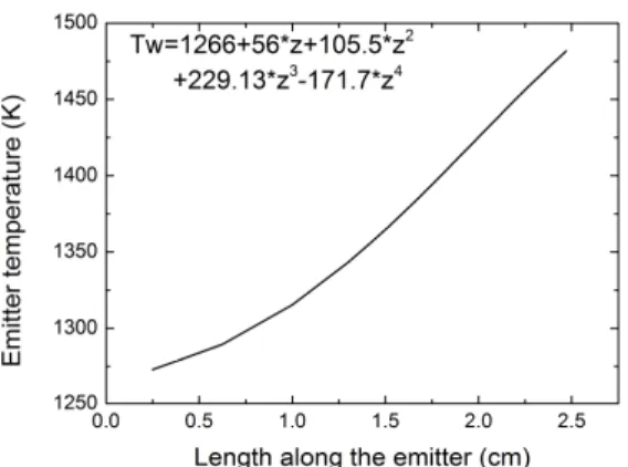
The temperature profile set to the emitter is shown in fig. 4. It corresponds to temperature measurements available in [2].

Figure 4: Emitter temperature profile set in plasma simulations of the cathode (no coupling to the thermal model) for the = 13  and = 3.6  simulation case. The downstream boundary of the emitter (closest to the orifice plate) is located at

an abscissa of 2.5  on the figure. The polynomial expression written here is used to specify the emitter temperature as a function of the normalized length along the emitter.

In this paper we will focus on a comparison between the simulated quantities (plasma density, plasma potential, electron temperature) along the centerline of the cathode and their experimental counterparts. A physical analysis of the plasma inside and outside the cathode is saved for our companion paper [17].

3 4 5 6 7 8 9 10 11 12 13 14 15 16 17 18 19 20 21 22 23 24 25 26 27 28 29 30 31 32 33 34 35 36 37 38 39 40 41 42 43 44 45 46 47 48 49 50 51 52 53 54 55 56 57 58 59 60

Figure 5 shows a comparison of the simulated plasma density and plasma potential to measurements available in the literature for the NSTAR cathode. Two simulated cases are shown on each plot, depending on the assumption of either a porous ( = 2) or nonporous emitter ( = 1) (see section II.B.1).

(a) _(b)

Figure 5: Comparison of the simulated plasma density (a) and plasma potential (b) to experimental measurements along the axis of the NSTAR cathode at = 13  and = 3.6  [13]. The influence of the porosity of the emitter ( = 2)

vs the non-porous case ( = 1) is also shown.

The simulated plasma densities inside the cathode for both simulation cases (either with or without a porous emitter) shown in fig. 5 (a) are in good qualitative agreement with experimental measurements. Compared to the non-porous emitter case ( = 1), the simulation with a porous emitter ( = 2) shows a steeper plasma density gradient towards the cathode inlet (decreasing abscissas in fig. 5) and the plasma is more tightly localized close to the orifice. In the simulation case = 2, in the interior region of the cathode, the difference between the simulated and measured plasma density is close to experimental error bars.

In the plume, the simulated plasma density for both cases ( = 1 and = 2) is almost identical and drops much faster than experimental measurements in the downstream direction. This difference is most certainly due to the lack of an applied axial magnetic field in the simulation, which confines the electrons in the radial direction (i.e. the anode direction) in the experimental setup. In simulations of the same cathode under the same operating conditions in which the applied magnetic field was accounted for, Mikellides et al. showed much better agreement with the plume density measurements [3]. Yet we will see in section IV that the excitation of plasma instabilities in the plume may cause an increase in plasma density there as well, even in the absence of an applied magnetic field.

The simulated plasma potential profiles for both simulation cases (fig. 5 (a)) are qualitatively different from experimental measurements. Inside the cathode towards the gas inlet, the simulated plasma potential for both 3 4 5 6 7 8 9 10 11 12 13 14 15 16 17 18 19 20 21 22 23 24 25 26 27 28 29 30 31 32 33 34 35 36 37 38 39 40 41 42 43 44 45 46 47 48 49 50 51 52 53 54 55 56 57 58 59 60

cases drops quasi-linearly with the distance from the orifice along the centerline, while measurements data exhibit a plateau. The approximate treatment of the emitter porosity ( = 2) alone cannot be blamed for the disagreement between simulated profiles and measurements, as it only increases the slope of the plasma potential which is already visible in the non-porous case ( = 1). We note that both a similar slope of the plasma potential along the axis in the non-porous case and its steepening when porosity is taken into account were observed in earlier simulations available in the literature for this cathode and this operating point [8]. Even if a more sophisticated model of the porosity was presented and used in [8], simulation results for the plasma potential remained in strong disagreement with experimental data available in [13]. We also observe that in measurements [13], the shape of the plasma potential in the interior region of the cathode seems to depend on the operating point: whereas a plateau is observed when the discharge current is set to = 13.1  , a linear decrease along the cathode axis is measured for a discharge current of 8.2 . Regarding this specific feature of the plasma potential in the = 13.1  case, both the model accuracy and experimental data may be questionable though. Indeed, Mikellides et al. noted in [37] that while a qualitative difference is observed between the simulated electric field deep inside the NSTAR cathode and available data, the very same model produced a good agreement with experimental data that includes measurements of , and obtained for a similar in design but larger hollow cathode (the NEXIS hollow cathode). This gives credit to their cathode model and sheds some doubt on the interpretation of experimental data in this region. We argue below, based on our current understanding of the cathode, that the experimental data for the plasma potential deep inside the NSTAR cathode does not follow the qualitatively expected trend. We also suggest a potential source of error in our model if measurements are indeed correct.

In the plume of the cathode, the simulated plasma potential profile differs as well from measurements. Both simulation cases display a non-monotonous evolution of the plasma potential along the centerline of the cathode, whereas the measured plasma potential steadily increases towards the plume. The discharge potential at the anode is moderately affected by the porosity of the emitter: with the discharge current set to = 13  , its value is 11.8  in the = 1 (non-porous) case vs. 10  in the = 2 case. A drop in the discharge potential was expected in the = 2, as the larger apparent emissive surface leads to a larger emitted current (since the emitter temperature profile is set). A smaller fraction of the total emitted current electron needs to be extracted and thus, the sheath potential which limits the electron current falling back on the walls needs not to be so high as in the = 1 case: the maximum sheath potential in front of the emitter is 4.9  in the = 2 case vs. 7.9  in the = 1 case. Hence the lower discharge potential.

3 4 5 6 7 8 9 10 11 12 13 14 15 16 17 18 19 20 21 22 23 24 25 26 27 28 29 30 31 32 33 34 35 36 37 38 39 40 41 42 43 44 45 46 47 48 49 50 51 52 53 54 55 56 57 58 59 60

It is certain that accounting for the applied magnetic field in the model can alter radically the plasma potential profile in the plume (as will be shown in our companion paper [17]), and lead to a better agreement between simulation results and experimental data. However, as it has been shown in past work by Mikellides et al. [3,35], other phenomena related to electron streaming instabilities in the plume may produce a time-averaged potential profile similar to the one measured for this cathode and shown in fig. 5 (b). This will be discussed below in section IV.

Lastly, we compare in fig. 6 the simulated electron temperature profiles (for both = 1 and = 2) to measurements [8,13]:

Figure 6: Comparison of the simulated electron temperature to experimental measurements for the NSTAR cathode at = 13  and = 3.6  [8,13]. The influence of the porosity of the emitter ( = 2) vs the non-porous case ( = 1)

is also shown.

Inside the cathode, the order of magnitude of the simulated electron temperature matches experimental data. However, the electron temperature decreases too steeply towards the inlet of the cathode (decreasing abscissas) in the = 2 (porous emitter) case w.r.t. to the measured trend, while the = 1 case is more similar to measurements (we neglect here the large experimental uncertainty w.r.t. the absolute electron temperature). It was suggested in [8] that the effective emissive surface of the emitter (the surface of the pores contributing to the emission) might be inversely proportional to the Debye length, in which case the value of should vary spatially (see the discussion below), and decrease towards the inlet of the cathode (see fig. 5 (a)). This could explain the better agreement between measurements and the simulated electron temperature profile in the = 1 case w.r.t. the = 2 case (once again, the experimental uncertainty on is neglected).

In the plume, the simulated electron temperature decreases as the plasma expands into vacuum, while measurements show an increase of the electron temperature. When compared with the simulated plasma potential profile (fig. 5 (b)) in the plume, it is tempting to conclude that the model presented so far lacks a 3 4 5 6 7 8 9 10 11 12 13 14 15 16 17 18 19 20 21 22 23 24 25 26 27 28 29 30 31 32 33 34 35 36 37 38 39 40 41 42 43 44 45 46 47 48 49 50 51 52 53 54 55 56 57 58 59 60