Combinatorial Incremental Problems
by
Francisco T. Unda Surawski
Submitted to the Department of Mathematics
in partial fulfillment of the requirements for the degree of
Doctor of Philosophy
at the
MASSACHUSETTS INSTITUTE OF TECHNOLOGY
September 2018
@
Massachusetts Institute of Technology 2018. All rights reserved.
41
~1
Signature redacted
A uthor ...
C ertified by ...
Accepted by....
MASSACUSETTS INSTITUTE OF TECHNOLOGYOCT 0
2
2018
LIBRARIES
Department of Mathematics
August 15, 2018
Signature redacted
Mich X. Goemans
Professor of Mathematics
Thesis Supervisor
Signature redacted
... ... . . . .
. . .
. .
Jonathan A. Kelner
Dhairman, Department Committee on Graduate Theses
Combinatorial Incremental Problems
by
Francisco T. Unda Surawski
Submitted to the Department of Mathematics on August 15, 2018, in partial fulfillment of the
requirements for the degree of Doctor of Philosophy
Abstract
We study the class of Incremental Combinatorial optimization problems, where solu-tions are evaluated as they are built, as opposed to only measuring the performance of the final solution. Even though many of these problems have been studied, it has' usu-ally been in isolation, so the first objective of this document is to present them under the same framework. We present the incremental analog of several classic combinato-rial problems, and present efficient algorithms to find approximate solutions to some of these problems, either improving, or giving the first known approximation guaran-tees. We present unifying techniques that work for general classes of incremental op-timization problems, using fundamental properties of the underlying problem, such as monotonicity or convexity, and relying on algorithms for the non-incremental version of the problem as subroutines. In Chapter 2 we give an e-approximation algorithm for general incremental minimization problems, improving the best approximation guarantee for the incremental version of the shortest path problem. In Chapter 3 we show constant approximation algorithms for several subclasses of incremental maxi-mization problems, including 2e_--approximation for the maximum weight matching problem, and a e-approximation for submodular valuations. In Chapter 4 we in-troduce a discrete-concavity property that allows us to give constant approximation guarantees to several problems, including an asymptotic 0.85-approximation for the incremental maximum flow with unit capacities, and a 0.9-approximation for incre-mental maximum cardinality matching, increincre-mental maximum stable set in claw free graphs and incremental maximum size common independent set of two matroids.
Thesis Supervisor: Michel X. Goemans Title: Professor of Mathematics
Acknowledgments
This thesis could not have been written without the support of many, many people. You know who you are. I would like to thank some of them, who had a particularly
big role in helping and encouraging me.
I would like to thank first and foremost my advisor, Michel Goemans, for infecting
me with his relentless courage to keep going, and despite his numerous other respon-sibilities, always finding time to meet with me. I cannot begin to recount how much he taught me about mathematics, but I will especially treasure our discussions about other aspects of life. I am also indebted to Jonathan Kelner and Ankur Moitra for serving in my thesis committee.
From MIT I would like to thank the many people I crossed paths or shared this time with, in particular to everyone in 2-390D. I would like to give a special thanks to Chiheon for the company during those long nights of writing.
I would also like to thank my girlfriend Annie, without whom this thesis would
not exist. Your encouragement and support through the hardest periods meant the world to me.
Finally, I would like to thank my parents, for their endless love and support. This is as much your achievement as it is mine.
Chapter 1
Introduction
In April of 2014, the water service pipe infrastructure in Flint, Michigan became contaminated with lead. What followed caught the nation's attention, including a 60% spike in deaths by pneumonia over the next two years, with twelve deaths attributed to Legionnaire's disease. Even more worrying were the long term effects. In particular, lead poisoning in children leads to developmental and health issues that would affect them for the rest of their lives. What happened is that officials failed to use corrosion-control treatment to maintain the integrity of the rust-layers in the pipes when switching the source of the water, and this meant that up to and maybe more than 15000 lead pipe lines were irrevocably contaminated and need to be replaced, and furthermore they will continue to pollute the water until they are. This infrastructure project has been estimated will take up to 15 years and tens of millions of dollars [31], [34].
This is exactly the type of optimization problem this thesis is about. We know we need to replace all the pipes, but it is not feasible to do it quickly. We must choose an ordering of the pipes to replace, and the goal is to minimize the total consumption of lead contaminated water over the timespan required to rebuild a clean water distribution network. The precise model to evaluate the lead intake for a partially rebuilt network would need to be formalized, but this crisis motivates the need for algorithms that optimize the order of decisions to be taken.
is often neglected. Usually the final solution is optimized, but heuristics are used in the implementation phase. This is a good approximation in the case where the total number of implementation time periods is small, but in many applications, a solution is implemented over the span of many time periods, either because it is costly to do
so, or because it takes time. In this thesis we explore one way of including this cost
in the optimization process, by limiting the parts that can be implemented at a time, and evaluating the partial solution at each time step.
1.1
Model and Preliminaries
There are of course many ways to model the incremental nature of a problem. One such way, is to have a budget for each time period, and a cost associated to changing the solution, and only allowing changes that stay within budget. In this case, we need to define what happens with any excess budget. One could allow rollovers, or maybe anything that is not used is lost. This of course depends on the problem. One could even allow budgets to become negative temporarily. On the other hand, the values we give our partial solution can be very complex, include discount rates or arbitrary weights for each time step. In this thesis, we derive results about a simple version. We model our solutions as subsets, and in each time step, we add exactly one element to this subset. The value we give to a solution on a given time step is a scalar function on these subsets, and the aggregated value of a solution is the simple sum of the values at each time step. Even in this simple case, we get very interesting problems, and furthermore, we get an insight into the extra difficulties one would run into by changing the model.
We adopt a common notation for all the problems. Namely, let E be a set of possible elements to be added to the solution, and v : 2E _ + be a valuation function. v measures some quantity of interest over subsets of E. We add elements from E one at a time, until there are no more objects to add. The general incremental
problem consists of finding a permutation a- : -+
{1,...,
E}
that optimizes|El
f(-) = v({e C E : o-(e) <i}). (1.1)
i=O
An instance of an incremental problem is encoded in the valuation function v. In many examples a single computation of the valuation v corresponds to the compu-tation of a solution of a classical combinatorial problem. For example, v might be the maximum matching of some initial graph augmented by additional edges. The focus will be in designing and analyzing algorithms for these incremental problems, whose performance depends on the general properties of the value v(-), rather than the specific optimization problem that corresponds to it.
We will divide incremental problems into incremental maximization problems and
incremental minimization problems. The reason for this is that the techniques we use
work very differently in each case. Formally, let's define
Problem 1 (INCR-MIN). Given a valuation
function
v E -+ Z+, find a permutation o- : E {1, . .. , IEI} that minimizes f (-).We define incremental maximization similarly.
Problem 2 (INCR-MAX). Given a valuation function v E -+ Z+, find a permutation
o- : E {1, . . . , IEI} that maximizes
f(-).
1.2
Literature Review
In terms of applications, this kind of optimization shows up in different ways. In a dis-aster scenario, a network or system is disrupted unpredictably and must be returned to its normal, optimal operation capacity (See for example [2], [3], [7], [22], 1231).
If the system is to be used throughout the reconstruction period, its capacity at
intermediate steps must be taken into account. The Flint water crisis is a specific ap-plication of disaster recovery. This is also related to the study of resilience of systems, the problem of ensuring amortized production/ efficiency level through disruptions. A
slightly different way in which incremental problems arise is when the implementation itself takes a long time, and hence one must be able to utilize a partially constructed system, i.e. the international space station is built in stages, but it would be an enormous waste of resources to wait until all its modules have been deployed. Long term projects are especially susceptible to this incremental problem paradigm, and can benefit from their optimization. B.J. Kim et al. propose in [21] algorithms to improve the investment plan for transportation facilities, noting even though the par-tial configurations are used for many years, this plan is usually created by optimizing the network at the planning horizon, and neglecting the intermediate states of the network. In
[251
and [28] the transformation of an electrical grid to a more modern form is studied. In [35] the same idea is studied for the design of transportation net-works. The authors incorporate uncertain demands to the planning information, and their valuation function also incorporates a discount rate for gains made in the future. Their solutions also includes expiration dates that have to be taken into account.The term incremental has been used to mean many different things in the litera-ture, in particular online problems. In these it is usual to assume that the revelation of information is adversarial, whereas the incremental problems treated here are full-knowledge, and the difficulty lies mainly in the optimization. The incremental flow problem was presented first by Hartline and Sharp [17], where they present a model where capacities increase, and there is a notion of hierarchy between consecutive flows. That is, for each edge, the flow on that edge may only increase. On a similar vein, Hassin et al. [18] introduce a version of the incremental maximum weight matching in which the solution is an increasingly larger matching, such that the min(k, MI) heaviest edges are close to a maximum weight matching with k edges. Fujita et al.
[15]
extend this notion to matroid intersection, and Kakimura et al. [19] to the knapsack problem. In this version, a knapsack solution needs to be computed such that the k heaviest objects in the knapsack are close to the optimal solution with k objects. A different notion of incrementality for the knapsack problem is presentedby Codenotti et al. in [91, where they include a notion of hierarchy in the objective
to a tree structure. Disser et al. [10] and Megow et al. [26] study a third notion of incremental knapsack. In this problem it is necessary to find a sequence of objects such that the solution that puts as many as possible in this order is close to optimal for any knapsack capacity.
The model of incremental problems considered in this thesis with its notion of aggregate costs has been studied for the particular cases of maximum flows [20], shortest paths
[41
and maximum weight spanning trees[14],
with a special focus on the performance of two natural greedy heuristics, Increment and Quickest-to-Ultimate. In the first one, one repeatedly finds a smallest set that increases the value of the solution, and in the second one, we find a set that maximizes the solution globally, and then apply Increment within this set. We generalize Quickest-to-Ultimate into something we call Multi-Point, and apply it to general incremental problems. In [20] Kalinowski et al. study the incremental maximum flow problem, and show that in the case of unit capacities, these greedy algorithms are constant approximations. In [4], Baxter et al. show a 4-approximation to the incremental shortest path problem, and that Quickest-to-Ultimate and Quickest-Increment can fail to be constant approximation algorithms. In[14],
Engel et al. study the in-cremental minimum weight spanning tree, and show that both Quickest-to-Ultimate and Quickest-Increment optimally solve this problem. This is due to the underlying matroidal structure as we point out in Section 1.3.Also related to the work presented here, Lin et al. [24] study a class of NP-hard incremental maximization problems, including k-means, the k-MST, k-vertex cover, and the k-set cover problems. In the k-means problem one wishes to choose a subset of k facilities to open to minimize the service cost for some set of customers. In the incremental version, we want to find an ordering of k facilities, such that for each
j
< k the firstj
facilities chosen are close to optimal for the corresponding j-means problem. In the k-MST problem, we are given a weighted graph and we wish to find a minimum-weight subtree that covers k vertices. In the incremental version, we wish to find a sequence of edges such that the smallest prefix that connects k vertices is close in weight to the optimal solution of k-MST. In the k-vertex cover problem, wewish to find a set of vertices of minimum weight that covers at least k edges. In the incremental version, we wish to find an ordering of vertices, such that the smallest prefix covering k edges is close in value to the optimal solution of the k-vertex cover problem. The aggregate measure of value Lin et al. use is the largest ratio between a hierarchical solution (i.e. given by the ordering) and the optimal solution to the car-dinality constrained problem, which is called the competitive-ratio in the literature. In contrast we use an average measure, where we compare the sum of performances of an ordering against the average performance of optimal solutions. Their stronger notion of performance requires an additional assumption, which they call the aug-mentation property of a problem. This allows them to grow partial solutions without increasing the cost too much. Our result in the first Chapter bears similarities with the competitive ratios that they find for exponential randomized algorithms, since they use the same techniques to prove it.
In [61, Bernstein et al. study the best competitive-ratio of cardinality constrained incremental maximization problems that have monotone and sub-additive valuations, including maximum matching, knapsack and covering problems. They also require the valuations they study to have a property they call accountability, which informally means that solutions can be devalued slowly, i.e. there are elements one can remove from the working solution that will not decrease it its value by too much. They also study the performance of the greedy algorithm which takes the element that increases the valuation the most each time, under a weaker version of submodularity.
1.3
Complexity and approximation
Most of the problems that we are interested in are either NP-hard in their original, non incremental version, or will become NP-hard when we include the extra robust-ness required by the incremental paradigm, and hence we are interested in efficient approximation algorithms. That is, we look for algorithms that are polynomial time, and give not necessarily the optimal solution, but a provably good one.
edges of a directed or undirected graph G = (V, E0 U E) with capacities on its edges,
and v(F) represents the maximum flow value from s to t (where s, t
C
V) in thecapacitated graph (V, E0 U F). The NP-hardness of this incremental problem was
shown by Nurre and Sharkey [30], see also Kalinowski et al. [201.
On the tractable side, the incremental optimization problem (INCR-MAX) can be solved efficiently if v(F) represents the weight of a maximum-weight independent subset of F in a matroid M with ground set E. Indeed, an optimum permutation can be obtained from a maximum-weight independent set B for the entire ground set E in the following way. First, order B in order of non-increasing weight followed
by all elements of E
\
B in an arbitrary order. This follows from the optimality ofthe greedy algorithm for matroid optimization and the fact that the truncation of a matroid is also a matroid. In the case of the incremental spanning tree problem, this was derived also in [14].
We focus on efficient multiplicative approximation algorithms. For a maximization problem, we talk about an a-approximation algorithm when the value of the solution found is always at least a times the value of an optimal solution, and for minimization problems, this value is at most a times the value of an optimal solution. In other words, for maximization problems, we have a < 1 and for minimization problems we have a > 1.
1.4
Overview
Throughout this thesis we assume two basic properties of our valuation functions, and at first we consider algorithms that work under these, but have no other requirements. In the case of minimization, this is enough to achieve constant approximation guar-antees, but not in the case of maximization, where we need further assumptions. The first condition is that valuations are monotonically non-increasing (non-decreasing) for minimization (maximization) problems. This is justified in many applications. The second assumption is a computational one. We require oracle access to v(-), that is, we have access to an oracle that outputs v(S) when given S. Furthermore,
we assume we can constructively approximate the optimum value of v(S) under a cardinality constraint IS < k. That is, we can find in polynomial time a set T such that v(T) approximates
mk := min{v(S) : S k},
for minimization problems, and the analogous maximization problem in that case. These values serve as a reference, since for any permutation, the value of a solution at step k is bounded by Mk, and in the analysis of the algorithms we design, we typically compare the value of the solution the algorithm produces to Ek nk. Our (approximate) oracle for mk is used as a black box in our generic algorithms, and we only argue about the implementation of this oracle when dealing with specific problems. We present algorithms and approximation guarantees in the most generic form possible, and then refine them for more restricted classes of problems, hereby improving the approximation guarantees.
1.4.1
Incremental Minimization
We start by considering generic incremental minimization problems in Chapter 2. We use ideas from Goemans and Kleinberg in [161 to design an algorithm for incremental minimization. The work in [161 concerns the minimum latency problem, with points in a metric space. There is a special point called a depot, and one wishes to find a tour from the depot to the rest of the points that minimizes the average travel time to each point. Goemans and Kleinberg make use of the fact that it is possible to find approximately shortest tours that visit k points, and by solving an appropriate shortest path problem, concatenate a subset of these to find an approximately optimal global tour. Using these ideas, we design an e-approximation algorithm for the general incremental minimization problem under very mild conditions, where e = 2.7182....
This is stated in Theorem 2.1. In particular, we show it improves the constant of approximation for the incremental shortest path problem from 4, found by Baxter et al. in
[4]
to e. An instance of the incremental shortest path problem is given bya weighted graph G = (V, EO U E, f) along with two special vertices s, t E V, and v(F) equal to the minimum length of an s-t-path using edges of EO U F. Baxter
et al. showed that this problem is NP-complete and that simple greedy heuristics fail to yield constant approximation algorithms. We also show in Section 2.2.2 that there are instances of the incremental shortest path problem for which our algorithm cannot approximate better than e asymptotically, and also that in some polynomially solvable instances studied in [4], namely that of disjoint paths, our algorithm returns the optimal solution. We also show that there are instances where the lower bound
Ek mk is a factor of e away from the optimum. This is described in Theorem 2.3.
1.4.2
Incremental Maximization
For generic maximization problems, we show in Chapter 3 that a simplified version of the techniques used for minimization provide a 0(1/log IE1)-approximation guar-antee.
Additionally, in Section 3.3 we show that for the incremental maximum weight matching problem there is a simple algorithm that yields 1 of the trivial upper bound
(1
+ IEi)v(E). We call this type of algorithm a 6-ratio algorithm (here for 6 = j), andwe show in Section 3.2 that by applying the techniques from Chapter 2, we can amplify such an algorithm into a e( -approximation algorithm. In particular, we show that the maximum weight matching problem has a 2- -approximation algorithm. As far as we know, this is the first constant approximation for the incremental maximum weight matching problem for general (not necessarily bipartite) graphs.
At the end of this Chapter, in Section 3.4, we discuss the case of submodular valuations. In this case the greedy algorithm already yields a ('-')-approximation to the cardinality constrained maximization problem, and hence to Mk, as shown by Nemhauser et al.
[29],
and this is best possible, but interestingly one can improve the constant of approximation for the incremental problem to e . This is done in Theorem 3.5.1.4.3
Incremental Cardinality Maximization
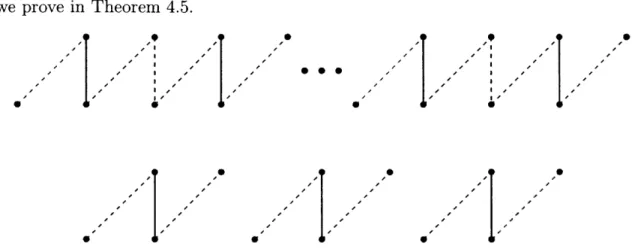
In the Chapter 4 we study cardinality maximization problems. In Section 4.1 we add two properties to our valuations, that are commonly found on cardinality maximiza-tion problems. The first property states that a valuamaximiza-tion can increase by at most one in each time period. The second one is a discrete-concavity property, whose discovery and application to the approximation of incremental problems is the main contribu-tion of this work. We will postpone the precise definicontribu-tion of discrete-concavity to Section 4.1, but we illustrate it here on the maximum cardinality matching problem. Suppose adding a set of edges S to a graph, the maximum cardinality of a matching increases by two. Then discrete-concavity asserts that there must be a set of size at most Lf that increases the maximum size of a matching by one. This can be shown by2 looking at the symmetric difference of two maximum matchings M and N that differ
by two:
|MI
=|NI
+ 2. This symmetric difference must consist of a disjoint set ofpaths and cycles, and at least two paths must be N-augmenting. By choosing a path appropriately, and adding these edges first in the permutation, we can guarantee that the matching increases by one by using at most half the edges of S. This property generalizes with 2 replaced by any integer k > 2.
In Section 4.2 we describe a simple asymptotic -approximation algorithm for general discrete-concave valuations, and in Sections 4.3 and 4.4 show how to get an asymptotic 0.85-approximation without further assumptions, by using a small geometric result about concave functions in [0, 1]. This leads to the best known guarantees for the incremental maximum flow with unit capacities, an improvement from 2 in [20], in the regime v(E) -+ oc. This is discussed in Section 4.5.
In Section 4.6 we focus on certain valuations that arise from independent sys-tems, and show that in this case concavity arises naturally from the integrality of certain polytopes related to feasible solutions, when one adds a cardinality constraint
(Theorem 4.3). For example, take the matching polytope
where X(M) is the characteristic vector of M. If we intersect PM with a cardinality constraint
{x
: E, xe = k}, one can show that the vertices of the resulting polytoperemain integral. We show this implies the discrete-concavity property. We exhibit several examples where the discrete-concavity condition is met by this polyhedral condition, including matchings, the family of independent sets in claw-free graphs and the common independent sets of two matroids (Sections 4.7, 4.8 and 4.9 respectively). In Theorem 4.5 of Section 4.10, we show that for independent systems there is a 0.9-approximation algorithm. Furthermore, we show that this bound is tight and we provide instances of the matching that achieve this approximation guarantee.
Kalinowski and Matsypura [20] study the same algorithm for the incremental maximum matching problem for bipartite graphs. In particular, they show that Quickest-to-Ultimate (Q2U) is a -approximation for this problem. Their tech-niques are polyhedral, and rely on the inequalities of the bipartite matching polytope. This improves the approximation guarantee for the incremental maximum cardinality matching problem to 0.9, and also generalizes it to several problems, including the maximum cardinality matching in general graphs.
1.5
Summary of Approximation Guarantees
Here we present a summary of the approximation algorithms contained in this work and how they compare to the state of the art, where a is the approximation guarantee for constructively computing mk as in Section 1.4. That is, we assume there is an algorithm that approximates mk to a factor of a. In Chapter 4 we assume a = 1.
Incremental Known Reference This work Section
Min General - - ae 2.1
Shortest Path 4 [4] e 2.2
Max Weight General - - O(a/ log(q)) 3.1
6-ratio j - max
{e
6 3.2Matchings - - 2e1 3.3
Submodular 1 - [29] e 3.4
__ _ __ __ _ __ _e_ _ 1+e
Card. General - - 4.4
Unit Max Flow 2 [20] (m-1) 4.5
3
Indep. System -
-Matchings [20] 9+_ 4.10
Stable Sets -
-Chapter 2
Incremental Minimization Problems
Incremental models have gained popularity in the last years, because of their practical applications to network design problems, disaster recovery, and planning. To mention some examples, Baxter et al.
[41
study shortest paths, Engel and Kalinowski1141
span-ning trees, Kalinowski and Matsypura[201
maximum flows and Nurre and Sharkey130]
the case of scheduling. This is of course not an exhaustive list. In this Chapter we use a technique first derived in [16] by Goemans and Kleinberg, to design a general purpose algorithm for a large class of minimization incremental problems. In116]
the authors design an approximation algorithm for the minimum latency problem or traveling repairman problem, a variant of the traveling salesman problem. In the minimum latency problem, we have customers in need of a repair, represented as points in a metric space. There is a special point called a depot, and we are tasked with finding a tour for the repairman that minimizes the average distance traveled from the depot to a customer. To provide an approximation guarantee, Goemans and Kleinberg use the solution to the related problem of finding an (approximately) shortest tour visiting k customers. They then concatenate some of these to obtain a tour with low latency, and the choice of which ones to use is given by the solution of an appropriate shortest path problem. We use this idea to design an e-approximation algorithm, which we call MULTI-POINT, that works for general incremental mini-mization problems. Then we look at how this algorithm is applied to the incremental shortest paths problem, where we improve on the best known approximationguaran-tee of 4
[4].
We also show that the lower bound used in the analysis of MULTI-POINT can be arbitrarily close to a factor of e away from the optimum even in the disjoint paths case. Finally, we exhibit a class of instances showing that the value of the solution returned by MULTI-POINT is arbitrarily close to e times the optimal value.2.1
A general algorithm
We derive an approximation algorithm for INCR-MIN that satisfies two basic assump-tions. First, we assume that adding more elements of E doesn't worsen our solution. In other words, we assume the function v is non-increasing:
Assumption 2.1 (NON-INCREASING).
VS C T : v(S) > v(T).
Now, we need a way to measure our progress, but in a way that can be computed without knowledge of the optimal sequence of solutions. Define mk to be the best value of any solution that uses at most k new elements. That is
mk = min{v(S)I S c E,|SI < k}.
Our second assumption is that these values can be efficiently either computed or ap-proximated. Specifically, we assume we have access to an a-approximation algorithm
A, which for each k returns in polynomial time a set Ek C E such that
I
Ek I = k andmk v(Ek) < amk. If a = 1 this is an exact algorithm.
Assumption 2.2 (COMPUTABILITY). There is a constructive a-approximation A
for Mk .
Note that the values rnk := v(Ek) can be assumed to be non-increasing by our
monotonicity assumption regardless of the algorithm A used to compute them. To see why that is, suppose we have computed two sets Ei and Ej such that i < j, JEiJ = i and
IEjI
= j, but v(Ei) > v(Ej). Then we can replace Ej by Ei U {x}, where x is anyelement of E \ Ej. By monotonicity we have v(Ej U
{x})
< v(E). Also notice that,for any ordering of the elements of E, when we add the k-th element, the value of the partial solution is at least mk. This implies that a lower bound for any solution is
q
LB = Em, (2.1)
i=O
where we define q :=
IEJ
throughout this thesis. Following the ideas from the la-tency problem, we consider using the partial solutions that come from computing an approximation nk and concatenating them. On the one hand, if we only want to minimize the value at step k we would take the optimal set with k elements. Simply add the elements of such a set in any order, and at the k-th step we will reach the minimum value possible. But on the other hand, we cannot simply use all of these sets, since they don't necessarily form a chain of containment. We strive to achieve a balance between these two opposing forces by considering a sequence0=-io <ii <... <if < it+, =q,
and for each
j
= 1, ... , E+1, computing Ei, <- A(ij). We proceed to add the elements from Ej, first, then from Ej2, etc., until we have added Ei, = E. As we add theelements from Eij we have already added all from Eij_,, Eij_2, etc., so we only need
to add e2 :=
1E
2,\
(Us<jEi,)I
elements. Note that ej < i3. Furthermore, since wehave already added all elements from Ei,_,, we know the value of our partial solution is at most ___,. All these facts together mean that the value of this algorithm is at
most
ejfij-, + fnq = ejsi,_ + (q + l)in-q < ijss 1 + (q + 1)ffiq =: UB, (2.2)
j=1 j=1 j=1
where si = mni - ?q > 0 and we have used for the first equality the fact that there
Observe that the bound on the right is pretty naive, since it is entirely possible, and likely in many cases, that when we add elements from Ei,, it is no longer necessary to add some elements from Ei, to decrease the value of a partial solution to the desired value. Despite this, we will show that this approach yields a constant approximation ratio for INCR-MIN. We haven't said anything about the choice of ii, i2,..., it, and we can optimize over this choice using the following lemma.
Lemma 2.1. Given any non-increasing set of numbers so si > ... > sq > 0, there
is a subset indexed by 0 = io < ii < ... < ij+1 = q such that
q ijsi _ < e ( sk, (2.3)
j=1 k=O
where e = 2.718... is the base of the natural logarithm. Moreover, such a subset can be found in polynomial time.
Proof. We assume without loss of generalization that sq = 0, since it doesn't appear
on the left hand side. We begin by showing the last part. Indeed the smallest value of the left hand side can be found as the length of the shortest path in the following graph. Let V = {0,... q}, and define directed edges (i, j) for each 0 < i < j < q,
with length
jsi.
Then the left hand side corresponds to the length of a path from 0 to q given by 0 = io < ii < ... < zj < it+1 = q, and the shortest of these paths can be efficiently computed. To show that the length of the shortest path satisfies the inequality, we use the probabilistic method. We take a random path, and show that, in expectation, its length satisfies the inequality. To do this, note that since sq+1 = 0,we can write
q q q-1 q-1
Sk = (sj - sj+1) = Z(sj - sj+)(J +
k=0 k=O j=k j=O
and similarly we have
f+1 f+1 q-1 q-1 k
E ijsi 1 = E (sk-sk+1) = (sk - Sk+1) ij,
where
jk
= max{j > 1 : ij1 k}. Therefore, we can rewrite inequality (2.3) asq-1 k q-1
Z(sk - Sk+1) Z 2j e (sk - sk+1)(k + 1).
k= j=1 k=O
Since the sequence {sk} is a non-increasing, to prove the above inequality it suffices to show that for every k:
9k
> e(k +1).
j=1
Following the ideas of Goemans and Kleinberg we take for j > 1, ij =
[Loei-1J
as long as this is less than q, and where 1 < L0 < e. Notice that indeed ij < ij+1 for allj >
1. Then the sum in question is 9k =i
[Loe'-j=1 Jk -1 ejk < Lo E e < Lo-e - 1 j=0 (2.4)Since ij = [Loej-1] we have
3k -- In k - + 1,-)
I(Lo
and so if we take L0 = eU, with U
C [0, 1], we have from inequality (2.4)
E< 1 ij Loeik
(k+1) -(e-1)(k + 1) (e ) ef(U)
where f(U) = [In(k + 1) - Ul - (ln(k + 1) - U) is a bijection in [0, 1].
(2.5)
Now we
randomize our path, by taking U to be a uniform random variable in [0, 1]. The distribution of f(U) is also uniform in [0, 1] and so by taking expectation in both sides of (2.5) we obtain
E
(
k+1
)
< (e e-e -11 E(eU) lne) =e.In(e)Finally, by linearity of expectation, this shows that inequality (2.3) is satisfied in
expectation, and so there must be at least one path that satisfies it.
Using this lemma and the previous discussion, we can already derive an approxi-mation algorithm for monotone minimization incremental problems. This algorithm is described in Algorithm 2.1, and we refer to it as the MULTI-POINT algorithm.
Algorithm 2.1: MULTI-POINT algorithm for INCR-MIN
Input A non-increasing valuation function v, and an a-approximation
algorithm A for Mk.
Output: A permutation -of E
1 Compute the values Pni = v(Ei), for i = 0, ... , q, using Ej <- A(i);
2 Construct the graph described in Lemma 2.1 for Si = Ti - Mq, and compute a
shortest (0, q)-path, given by 0 = io < i < ... < it+, = q;
3 Output -consistent with how elements appear in the sequence Ei, .... EV,.
We observe that there is nothing random about MULTI-POINT, despite the proof of Lemma 2.1 being probabilistic. This algorithm has an ae approximation guarantee.
Theorem 2.1. MULTI-POINT(2.1) is an ae-approximation to INCR-MIN for
non-increasing v. In particular, if it is possible to compute the values mi exactly, MULTI-POINT is an e-approximation algorithm.
Proof. Note that the algorithm doesn't completely define the permutation, since it
is possible that several choices of sets E exist, and also the order chosen within sets is ambiguous. Let ALG be the worst possible value attained by a permutation consistent with Algorithm 2.1 and let OPT be the optimal value of f(o-). Finally, for the sequence chosen by the algorithm 0 < ii < ... < it+1 = q we have seen in (2.2) that the value of the solution returned by the algorithm is at most
ei
UB = i (iii-3 1 - fnq) + (q + 1)'fq.
j=1
On the other hand, we have seen in (2.1) that the value of the incremental problem is bounded from below by
q-1
LB= Z(m - mq)+(q+1)mq.
i=0
Hence it is clear that
LB<OPT<ALG<UB.
Lemma 2.1 implies that
q-1 q
UB < eZ(fi - g)+ (q+ 1)gfq e Eiiq.
i=O i=O
and hence the approximation guarantee of A implies
q
UB < ae mi < aeLB,
i=o
hence
ALG < UB < aeLB < aeOPT.
We end this section by observing that if one has access to a polynomial time approximation scheme (PTAS) to compute Ek such that v(Ek) approximates mk, i.e. a class of algorithms
{A
0}
parametrized by a > 1 such that for any given a > 1,Ac runs in polynomial time (where the exponent may depend on a) and produces a
solution within a of optimum, one has the following result.
Corollary 2.1. If {A0} is a PTAS which outputs a set Ek such that Mk < v(Ek)
aMk, then by taking a = 1+e/e for an arbitrary E > 0, MULTI-POINT is a polynomial
(e + e)-approximation algorithm for the incremental minimization problem.
2.2
Incremental Shortest Path
The classical shortest path problem is, given a graph G with a length function on its edges and two vertices s and t of this graph, to find a shortest path from s to t. The graph can be directed and weighted in the general case.
An instance of the incremental shortest path problem is given by I = (V, E0, E,
)
and t : Eo U E -+ Z+ is the length or cost of an edge. We assume that s and t are connected by a path made from edges of E0. Let v : 2E -+ R be the shortest (s,
t)-path function, i.e. v(S) is the length of the shortest t)-path using edges of E0 U S. The
incremental shortest path problem consists of finding a bijection -: E -+ {1... .
IEI},
that minimizes
|El
i=O
We now show that there is a pseudo-polynomial transformation to reduce any instance into an unweighted one. Indeed, replace each edge of E0 of weight f(e) by a path
of length f(e) of edges of E0, and each edge of E by a path of length f(e) where all
but one of the edges is in E0. Any algorithm for the unweighted case can be applied
efficiently in this transformed instance, with the same guarantees. The new graph has e, f(e) edges, so if we have a polynomial algorithm for the unweighted case, we can naturally apply it to the weighted case, and it will remain polynomial as long as the number of edges grows polynomially. Since this is a minimization problem, we must assume that the initial graph has some path from s to t, otherwise, the cumulative cost will be infinite. Clearly the valuation v satisfies monotonicity. In
[4],
the authors show that this incremental problem is NP-hard to compute exactly, and they exhibit an algorithm that achieves a 4-approximation. They also show that mkcan be computed efficiently, i.e. there is a polynomial constructive 1-approximation
A, so by the results of the previous section we improve the approximation guarantee
from 4 to e. We observe that it was shown in
[41
that both Quickest-to-Ultimate and Quickest-Increment (see Chapter 4), and even the algorithm that takes the best between the two, fail to give a constant approximation guarantee for this problem.Corollary 2.2. Algorithm 2.1 is an e-approximation algorithm for the incremental shortest path problem.
2.2.1 MULTI-POINT is optimal for disjoint paths
In the case of shortest paths, we can say a bit more about some restricted cases. For example, in the case where the graph is a disjoint union of (s, t)-paths. Using the
notation of the proof of theorem 2.1, we show that in this case, MULTI-POINT returns an optimal solution. Following this, we show that there are instances where the lower bound LB (2.1) can be a factor of e away from the optimum, even in the case of
disjoint paths, suggesting that more powerful bounds would be needed to improve the approximation guarantee.
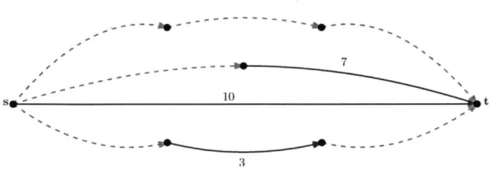
- 7
- 10 t
3
Figure 2-1: An instance of the incremental shortest path problem for disjoint paths. Red dashed edges are edges of E, and have zero length. Blue solid edges are edges of
E0, and their length is given.
In [41 it was noted that if the original instance is a disjoint union of s-t paths (see
figure 2-1), we can compute the optimum value in polynomial time. Indeed, we show
that MULTI-POINT (2.1) achieves this.
Theorem 2.2. MULTI-POINT returns an optimal solution for the incremental
short-est path problem in the case of disjoint paths.
Proof. Suppose G is made up of r +1 disjoint paths, each with qi edges from E and of length ci. We note that this completely characterizes a disjoint paths instance of the
incremental shortest path problem. It can be assumed that co > cl > ... > cr and 0 = q0 < qi < ... < qr. Note that algorithm A is trivial in this case; A(k) returns
the set of edges of E in the path with the smallest length that satisfies qi < k. Then the choice becomes that of which subset of these paths should we complete before reaching the minimum distance cr. Let 0 = ko < k, < ... < km = r be this choice of which paths to complete first. For each choice we need to add qk, edges to complete
the path, and achieve a length Ckj. Since we add them in order, this gives a valuation
edges from paths we didn't choose so the total valuation is
M kj-1 m
E qkjCk_ - Cr E q3 + = E qk, (Ck,1 - Cr) + Cr
j=1 ( s=kj-,+1 j=1
This was derived by Baxter et al. in [4]. Observe now that in this only if qj
<
i < qj+1, where we define q,+= qs. Suppose 0 = io < il < .,.. < it < it+1 = q is a subset of {0, q1, q2, ... ,qr+1}and qr+1. Then MULTI-POINT has an upper bound (2.2) of
( q,-1
s=1
case mi = cj if and now that the path that includes 0, qr
UB = ij(mi_ mq) + (q + 1)mq = E qk(Ck 1 - cr) + cr( q, +1
j=1j=1 s8=1
El
and hence delivers an optimal solution.
30
20
0 1 2 3
10
21
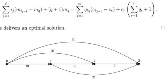
Figure 2-2: Finding the optimal ordering of potential edges in the incremental shortest path instance above corresponds to finding the shortest path in this auxiliary graph.
This shows that in the case of disjoint paths, MULTI-POINT is actually optimal (See Figure 2-2). Despite this, we can show that even in the case of disjoint paths, our original analysis cannot show a better approximation constant than e. In particular the lower bound (2.1) can be an e fraction of the optimal value. For this, let's look at a concrete instance.
Example 2.1. For each r, define 1, to be the following instance of the incremental
shortest path problem with disjoint paths. Let qi = i for i = 0,. . . , r, and ci = 1/i for
1 < i < r, co = 1 + E and c, = 0.
We will show that in this family of instances parametrized by r the ratio between the optimum value and the lower bound
Z?-
mi approaches e.Theorem 2.3. Let LB, be the value of the lower bound (2.1) for instance I, (Example 2.1). Similarly, let OPT, be the value of an optimal solution of I,. Then
OPT
L -+ e,
LBr as r - oc.
Proof. Let ALGr be the value of a solution returned by MULTI-POINT in instance Ir. We have mi = ci for i = 0,... , r, and mi = 0 for i > r. In particular, this means the
lower bound is bounded by
q r-1 1r-2 i+1 I -1I
Mi = 1+E E Z+ < 2+E+ dx = 2+E+ dx = 2+E+ln(r -1).
i==O ~ i=1 =
On the other hand, since MULTI-POINT returns an optimal solution, OPT has the form
ALGr = OPTr Z i(mii - mq)+ (q+ 1)m=q ijmTi,_,
j=1 j=1
for some choice 0 < i1 <i2 < ... < ij < q (Note that for disjoint paths, ej = ij). The
equality follows from noting that mq= Cr = 0. Now take
j*
= max{j 1i 1 < r}. Forany
j
>j*,
we have Zi_1>
r, and hence m = 0. On the other hand, forj
< j* we have mij_1 = ci_,. This means we havej*
OPT = ii(1 +E) +
L
> eln(ij.) > eln(r).j=2
-The first inequality can be checked by induction on j*: For x > 1, the convex function
x -+ x - e ln(x) achieves its unique minimum value of zero at x = e, and so if
j*
= 1,we have ii > r
>
e ln(r). In the induction step, we have3*
ii + ( ~ij1/_1 > eln(iz*i-) + Z-i-/ij-_1 > eln(ig.), j=2
where the second inequality becomes obvious when we write it as
ij./ij-_1 ;> e ln(ig./ij._1).
Note that OPTr/LB, = ALG,/LB, < e by Corollary 2.2. On the other hand,
e ln(r) - 2
+E
+ ln(r - 1)This implies that
OPT
LBr + e.
2.2.2
Worst-case example
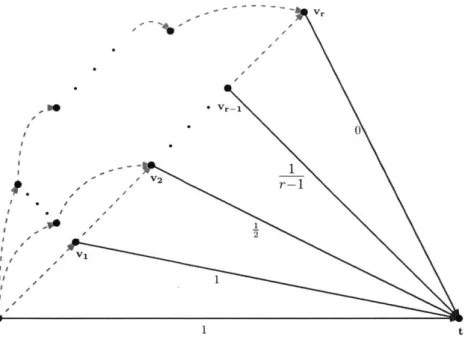
Even though we have just shown that the lower bound can be an e fraction of the optimum, it is not clear that the value of a solution returned by MULTI-POINT can be this large. In principle it is still possible that using a better lower bound we can improve the approximation guarantee of this algorithm. In particular, in Example 2.1 the optimum value and the algorithm coincide. We show that this is not the case, exhibiting a family of instances where the value of the algorithm is an e factor away from the optimum value. Consider the following instance (See Figure 2-3).
Example 2.2. Given r, let J, be the following instance of the incremental shortest
path problem. Let V = {s,t,V1,... ,Vr}. E0 consists of {s,t} and all edges of the
form
{vi,
t} where i c{1,...
, r}, and the potential edges E are{s,
vi}, and all edgesof the form {vi, vi+1}, where i = 1, ... , r - 1. Furthermore, for each 1 < i < r, add a
path P of i edges of E connecting s and vi. Finally, we let f(s, t) = 1, f(vi, t) = 1/i,
for i = 1, ... , r - 1, f(v,, t) = 0, and - 0 for every other edge.
Theorem 2.4. Let ALGr be the value of a solution returned by MULTI-POINT in Jr (Example 2.2), and let OPTr be the value of an optimal solution to this problem.
0 I V11 S t s r r-S 1 t
Figure 2-3: An instance showing that Algorithm 2.1 can't have a better than e ap-proximation guarantee.
Then
ALGr OPTr as r -+ 00.
Proof. It is not hard to see that the optimum in this case is to include the edges in
the order they were defined, which gives a value of
LBr =OPT + Z ; 2+ =j 2 -)
i=1
Now consider a solution given by the algorithm, i.e. a sequence 0 = io <e Kre ... K
eie i1= q. Observe that mo =1, m=1/i for i= 1, ... ,r - 1andrm =0for
i 2r. For each i3, the algorithm might use the edges from Ps, to achieve mi3, which gives a value of
A LGr ;> 41+
Ziay/ij-1
e ln(r),j=2
Hence, we have that this family of examples indexed by r satisfies
e>ALGr
OPT > -- 2+ln(r -1))'e 1) --(+r) e as r -4 o0
Chapter 3
Incremental Maximization Problems
We now turn our attention to incremental maximization. We show that the one point version of the MULTI-POINT algorithm is a (g )-approximation algorithm for the maximization problem. In the second part of this chapter we show that
by a more nuanced application of the techniques of Chapter 2 we can improve the
guarantees of some simple constant approximation algorithms, including a
(I
+I2)-approximation guarantee for the incremental maximum weight matching problem. In the third part of this Chapter, we show that if the valuation is submodular, the greedy algorithm is a ( e)-approximation algorithm. We observe that this is an improvement over the obvious (1 - ')-approximation algorithm that follows from the results of Nemhauser et al. in
[29].
3.1
General incremental maximization
We show that an algorithm, which we call ONE-POINT (See Algorithm 3.1), is a
logq)-approximation algorithm for general incremental maximization problems.
This is the one point version of the MULTI-POINT algorithm of the last Chapter. Our first assumption is that the valuation is non-decreasing:
Assumption 3.1 (NON-DECREASING).
As in the last Chapter, we define mk to be the best value of a solution that uses at most k elements. In the case of a maximization problem that corresponds to
mk = max{v(S) : S C E,ISI < k}.
Our second assumption, as before, is that we have access to these quantities. That is, there is an algorithm A, with an associated constant a < 1, such that A(k) returns in polynomial time a set Ek C E such that IEkI = k and amk < v(Ek) < mt.
Assumption 3.2 (a-COMPUTABILITY). There is a constructive a-approximation
algorithm A for Mk.
Observe that as before, if a = 1, we have an exact algorithm, and by the mono-tonicity assumption 3.1, the values fik := v(Ek) can be assumed to be non-decreasing.
Furthermore, we can assume that mio = mo and -q = mq, since A needs only return
0 and E respectively. For any permutation of E, the value of the first k elements of that permutation is at most Mk, so an upper bound to any solution is
q
UB =
mi,
(3.1)i=O
recalling that q = IE. Now suppose we pick one index 0 < i < q and compute using A a set E such that IE I = i and mi = v(Ei). If we add the elements of E first, we can guarantee a value of
P(i) = imo + (q - i)fi + Mq. (3.2) We show that optimizing over the choice of i already gives a non trivial approximation guarantee. We will need the following lemma.
Lemma 3.1. Given q 2, and a non-decreasing set of numbers 0 < t1 < ... < tq,
there is a choice of 0 < i* < q such that
(q + 1 - i*)ti. > H(q)-' ti, i=1
where H(q) = is the Harmonic Junction.
Proof. By taking i* maximizing (q + 1 - i)tj we obtain
q q (q +a 1- *
I
tj <_ (q. 1i) = H(q)(q +1 -i*)ti-,where H(q) = E I_ El
This immediately suggests an algorithm to approximate to order a/log(q) (where log is the natural logarithm) any incremental maximization problem with a non-decreasing valuation. This is the ONE-POINT algorithm and it is described in Algo-rithm 3.1.
Algorithm 3.1: One-Point Algorithm for incremental maximization of a
mono-tone function
Input A non-decreasing valuation function v, and an a-approximation
algorithm A for Mk.
Output: A permutation o- of E
1 Compute the values mj = v(Ej), for j 0,... , q, using Ej <- A(j); 2 Compute 0 < i* < q maximizing rii (q + 1 -0 )
3 Output any permutation -where all elements of Ej. come first;
Theorem 3.1. ONE-POINT is an Q ( -approximation algorithm to INCR-MAX,
with non-decreasing v.
Proof. This algorithm has value at least P(i*) (3.2), and by applying Lemma 3.1 to tj = fi, we obtain that the value obtained by the algorithm is at least
P(i*) > i*mo + (q + 1 - i*)fi%* > i*mo + H(q)-1 E >
i=1
H(q) 1 E ti,
i=O
where H(q) = Q(log(q)-1). Note that the case i* = q corresponds to taking an
arbi-trary permutation. Now, suppose OPT is the value of an optimal solution, and ALG the value of the solution returned by ONE-POINT. Since UB (3.1) is an upperbound
of OPT, we have
q q
ALG > P(i*) > H(q)-1 -i > aH(q)- Zmi > aH(q) OPT,
i=O i=O
hence
ALG > aH(q)-1OPT,
showing that ONE-POINT is an aH(q)-1 = 0 -approximation algorithm. E
3.2
An improvement for instances with high ratio
We now show an algorithm we call REVERSE-MULTI-POINT that improves the value given by another algorithm B. We require that the value of a solution given by B has a property we call -RATIO, which informally says that this value comprises at least a 6 fraction of the total possible. More precisely, note that the value of the algorithm at any point is bounded from above by mq = v(E). Since there are q + 1 steps in any
construction, the total value cannot exceed (q
+
1)mq. We say an algorithm satisfies the 6-RATIO condition if it returns a solution with value at least 6(q+
1)mq.Assumption 3.3 (6-RATIo). There is a polynomial time algorithm B with a 6-ratio.
We observe that this implies that B is a 6-approximation algorithm, since (q+)mq is, in particular, an upper bound on the optimal value. We will show that we can apply a version of the multi-point algorithm that we used for minimization, to improve the constant of approximation, provided we have a large enough a.
Fix a sequence 0 = io < ii < ... < it < if+1 = q, and use algorithm A to compute for each
j
= 1, ... , e+1, a set Eij such that |E, I = ii and f-ij = v(Eij) > amij. Addthe elements in an order consistent with how they appear in Eg1, E2, . .., and suppose
we add ej elements when adding set Ei,, i.e. ej = jEjj \ (Uj~4Ei) . Note that
ej = q and ej < i. Finally, recall that we assume that rnio = mo and fgq = mq,