HAL Id: hal-02272264
https://hal.archives-ouvertes.fr/hal-02272264
Submitted on 27 Aug 2019
HAL is a multi-disciplinary open access
archive for the deposit and dissemination of
sci-entific research documents, whether they are
pub-lished or not. The documents may come from
teaching and research institutions in France or
abroad, or from public or private research centers.
L’archive ouverte pluridisciplinaire HAL, est
destinée au dépôt et à la diffusion de documents
scientifiques de niveau recherche, publiés ou non,
émanant des établissements d’enseignement et de
recherche français ou étrangers, des laboratoires
publics ou privés.
THE INVERSE PROBLEM OF WAVELET SCHEME
CONSTRUCTION FOR IRREGULARLY
SUBDIVIDED 3D TRIANGULAR MESHES
Sébastien Valette, Yun-Sang Kim, Rémy Prost
To cite this version:
Sébastien Valette, Yun-Sang Kim, Rémy Prost.
THE INVERSE PROBLEM OF WAVELET
SCHEME CONSTRUCTION FOR IRREGULARLY SUBDIVIDED 3D TRIANGULAR MESHES.
QCAV, 2001, Le Creusot, France. �hal-02272264�
THE INVERSE PROBLEM OF WAVELET SCHEME CONSTRUCTION FOR
IRREGULARLY SUBDIVIDED 3D TRIANGULAR MESHES
Sébastien VALETTE, Yun-Sang KIM and Rémy PROST
CREATIS, INSA - Bâtiment Blaise Pascal 69621 Villeurbanne cedex
,
Francetel: 33 (0)4 72 43 82 27, fax : 33 (0)4 72 43 85 26, e-mail : {sebastien.valette, kim, remy.prost}@creatis.insa-lyon.fr
Abstract - We investigate a recent mesh subdivision scheme, allowing multiresolution analysis of irregular
triangular meshes by the wavelet transforms. We consider the wavelet scheme construction in terms of an inverse problem. Some experimental results on different meshes prove the efficiency of this approach in multiresolution schemes. In addition we show the effectiveness of the proposed algorithm for lossless compression.
1. INTRODUCTION
Multiresolution analysis of 3D objects is receiving a lot of attention nowadays, due to the practical interest of 3D modelling in a wider and wider range of applications and in particular in artificial vision. Multiresolution analysis of these objects gives some useful features : several levels of details can be built for these objects, accelerating the rendering when there is no need for sharp details, and allowing progressive transmission. Another feature is that multiresolution analysis can be an efficient way for data compression. A survey of the existing methods used to simplify meshes which is the first step for processing multiresolution analysis, like vertex decimation [2], edge contraction [3] and wavelet based analysis [4], was reported in [1]. We put our attention on the third method, because wavelets are well-suited for multiresolution analysis. In section 2, we will shortly explain multiresolution analysis of meshes [3], and show its drawbacks in practical implementation, which we extend for irregular triangular meshes. Based on a recent work [5] we consider the inverse problem of the wavelet scheme construction in section 3. In section 4, we show why our proposal is suitable for compression. Section 5 gives the results obtained with this new scheme.
2. LOUNSBERY’S WAVELETS BASED MULTIRESOLUTION SCHEME
In wavelets decomposition, a mesh (for example a tetrahedron, see figure 1.a) is quaternary subdivided (figure 1.b) and deformed (figure 1.c), to make it fit the surface to be approximated. Subdividing the mesh consists in splitting each triangular face into four faces. These steps can be processed depending on the required resolution levels.
a) b) c)
Figure 1: the subdivision scheme
Multiresolution analysis is computed with two analysis filters A and j B for each resolution level j .j
Reconstruction is done with two synthesis filters P andj
j
Q . Let us call C the 3j vj× matrix giving the
coordinates of each vertex of the mesh at the resolution level j . Then we have :
1 1. + + = j j j A C C (1) 1 1. + + = j j j B C D (2) j j j j j P C Q D C +1= . + . (3) j
D represents the wavelet coefficients of the mesh,
necessary to reconstruct Cj+1 from C . From aj
theoretical point of view, each column of the P matrixj
(respectively the Qj matrix) represents a scaling function (respectively a wavelet function). These functions are defined on a 3D space fixed by the mesh topology. We apply the lifting scheme [6] which consists in constructing wavelet functions, starting from the hat function, orthogonal to the scaling functions which are hat functions too, but with a twice wider support. Without the lifting scheme, Lounsbery's multiresolution analysis would simply consist in subsampling the mesh (these wavelets are known as “lazy” wavelets), but with the lifting, the mesh at resolution level j is ensured to be the best approximation in the mean square sense for the mesh at level j+1. The main material for the lifting is the inner product between two functions defined by Lounsbery as:
∑
∆∫
∈ ∈ >= < ) ( ). ( ). ( ) ( , M s j ds s g s f area K g f τ τ τ (4) ) (M∆ is the set of triangles τ of the mesh and Kj is a
constant for a given resolution level j . (Kj = 4 ). Note−j
that in this inner product it is assumed that the triangular faces of the mesh have the same area. The consequence of this assumption is that a mesh at resolution level j will effectively be the best approximation of the mesh at level
1 +
Wavelets give a powerful tool for multiresolution analysis of surfaces. However, in the simplification process, the major drawback is that faces are always merged four to one to have a simpler mesh. If the mesh does not respect this connectivity constraint, one has to process a resampling of the mesh, known as remeshing, which results in a mesh having more faces than the original, as explained in details in [7] and [8]. The aim of this work is to solve this problem by improving the subdivision process, as described in the next section.
3. A PROPOSAL FOR IRREGULAR MULTIRESOLUTION ANALYSIS
A. Avoiding the remeshing step
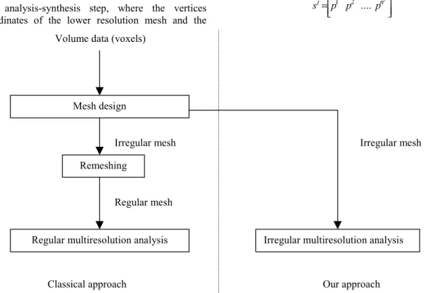
The aim of this paper is to provide a new method allowing to process multiresolution analysis directly on irregular meshes, avoiding the remeshing step, as shown in figure 2. This would result in two major improvements in multiresolution analysis on meshes:
- No extra computation is needed (for the remeshing) - The reconstruction of the mesh can lead to a mesh
identical to the original mesh. This allows a lossy to lossless encoding scheme for meshes.
Applying the multiresolution scheme on irregular meshes requires the modification of the two main steps:
- The subdivision step, which gives the relation between the different level meshes (connectivity) - The analysis-synthesis step, where the vertices
coordinates of the lower resolution mesh and the
wavelet coefficients are computed (geometry) These two modifications are described in details in the two next sections.
B. Modeling irregular subdivision scheme is an inverse problem
In the regular multiresolution scheme, the connectivity of all different level meshes depends on the lowest level mesh connectivity. Then the highest resolution level mesh connectivity has to be highly regular. Unfortunately, classically built meshes (e.g. meshes built with the marching cubes algorithm [9]), are not regular and can not be directly used.
As a result, the subdivision scheme has to be changed, in order to allow every mesh to be processed. Based on [5] we propose an enhanced subdivision process, where the subdivision differs from a face to another one.
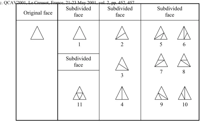
In our scheme, each face of a mesh can be subdivided in four, three or two faces, or remain unchanged. Figure 3 depicts the possible cases of subdivision for one face. The direct problem
Taking a mesh M having j n faces and j v vertices, wej
call S a subdivision scheme applied on it, representedj
by the a row vector s containing j n elements (integersj
between 1 and 11), and describes the subdivision case for each face: = nj j p p p s 1 2 .... Mesh design Remeshing
Regular multiresolution analysis Irregular multiresolution analysis Volume data (voxels)
Irregular mesh
Regular mesh Irregular mesh
Classical approach Our approach Figure 2: regular versus irregular wavelet scheme
1 +
j
M is then the result of the subdivision process:
1 + →S j j M M j (5) We define the efficiency ratior as:j
j j j n n r = +1 (6) Note that: 4 1≤rj≤ (7)
There are 11 possible subdivision schemes, but not allni of them lead to a manifold mesh, as shown in figure 4 : The subdivision of the two faces in figure 4-a) results in a manifold mesh, but the in figure 4-b), the result is non-manifold.
a) manifold result
b) non manifold result (marked vertice) Figure 4: The manifold constraint
The inverse problem
In order to apply multiresolution analysis by wavelet decomposition on a given mesh M , one shall find aJ
mesh MJ−1 and a subdivision scheme SJ−1 satisfying:
J J
J M M
S −1( −1)= (8)
This is a blind inverse problem. We can say that for any manifold mesh M , there always exist one meshJ
1 −
J
M and one subdivision scheme SJ−1 satisfying this
constraint. One evident solution is the identity subdivision scheme sident =
[
1 1 ... 1]
, which leaves the entiremesh unchanged:
J J ident M M
S ( )=
But Sident is not an interesting solution, resulting in rJ−1
equal to 1. In a coding efficiency purpose, one shall find a subdivision leading to a ratio rJ−1 as near as 4. This consists in merging the faces of the mesh M , leading toJ
a mesh MJ−1 having the lowest number of faces possible.
Figure 5 shows an example, where 15 faces are reduced to 6, resulting from merging 4 :1 faces for G2, 3 :1 faces for G3 and G6, 2 :1 faces for G1 and G4 and keeping one face unchanged for G5. For this subdivision scheme,
5 . 2 6 15 1 = = − J r .
Original face
Subdivided
face
Subdivided
face
Subdivided
face
Subdivided
face
1
2
3
4
5
11
6
7
8
9
10
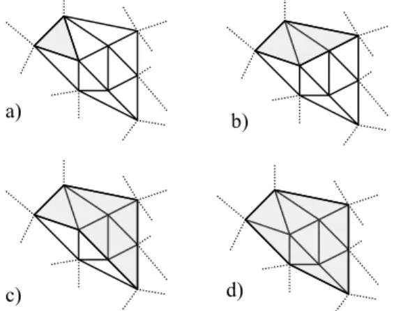
Figure 5: an example of mesh simplification Briefly, the proposed simplification algorithm starts by selecting one face, building a set of merged faces (which first consists in this selected face), and tries to expand this set by merging faces around it. Figure 6 shows the beginning of the expansion of the merged faces set (in gray), merging sequentially a) one face, b) 2 faces, c) 4 faces and d) 3 faces.
Figure 6: expansion of the simplified face set The algorithm stops when no more faces have to be merged. In order to prevent the algorithm from being unable to merge some faces with respect to the manifold constraint, a modification of the mesh is allowed. It consists in an edge swapping between two neighbour faces, as shown in figure 7. Of course this modification has to be stored, to recover the original mesh after subdivision and guarantee the reversibility of the simplification process.
Figure 7: an edge swap between two faces We notice that this modification will introduce a supplementary quality loss during multiresolution analysis, but the difference between the original mesh and the altered mesh is small and experimental results show that this local error is negligible compared to the approximation error. Finally, the algorithm is very efficient for simplifying a large set of meshes.
C. Filter-bank construction
The last thing to do is to compute the approximation of the high resolution mesh with the simplified one that is to calculate the analysis filters A and j B . This can bej
done with Lounsbery’s scheme. A difference has to be noticed, due to the change of the subdivision process. The inner product (5) has to be reformulated and becomes:
∑
∫
∆ ∈ ∈ >= < ) ( ). ( ). ( ) ( ) ( , M s j ds s g s f area K g f τ τ τ τ (9)Kj(τ) is no longer a constant and changes with each face
of the mesh. For example, a face in a low resolution mesh that will split in 3 faces will have Kj(τ)=3 and the three
resulting faces will have Kj+1(τ)=1, taking into account the
differences between the triangle areas : the first face cited above will approximately be three times larger than the three last.
4. COMPRESSION
A. Compression efficiency
The proposed method has powerful features for compressing meshes, for two reasons:
• The wavelet decomposition, used to compute the vertices coordinates, transforms coordinates into wavelet coefficients which histogram is concentrated around the zero value, making them well suited for entropy coding.
• Starting from the lowest resolution level, there is no need to store or transmit the faces descriptions to reconstruct higher levels, only the subdivisions have to be, which lets the amount of information needed to reconstruct the connectivity of the mesh close to 2 bits per face.
In the experimental results section, the lowest resolution mesh is not compressed.
B. Lossless compression of the vertices coordinates
Here we consider vertices with integer coordinates in order to perform lossless compression. In addition, a number of rounding operations have to be introduced in the multiresolution analysis-synthesis scheme. For a brief demonstration, one shall come back to the construction of the matrix filters Aj+1, Bj+1, P and j Qj used in equations (1), (2) and (3).
First, we introduce Alazyj+1, Blazyj+1, Plazyj and Qlazyj as the “lazy” filterbank. These filters do not perform any approximation, since during the analysis (where some vertices are removed, as the mesh is simplified) the coordinates of the remaining vertices stay unchanged. An integer-to-integer intermediate analysis-synthesis scheme can be defined as:
G1 G2 G3 G6 G5 G4 a) b) c) d)
1 1 intj ermediate =Alazyj+ .Cj+
C (10)
+1. +1
= j j lazy j B C D (11)
j j
lazy j ermediate j lazy j P C Q D C +1 = . int + . (12)where
. and
. are respectively the floor and ceiling operators, and ensure perfect reconstruction, as described in [10].The approximation-effective filter-bank directly derives from the “lazy” filter-bank modified by the lifting scheme: 1 1 1 1 + + . + + = + j lazy j j lazy j A B A α (13) 1 1 + + = j lazy j B B (14) j lazy j P P = (15) 1 . + − = j j lazy j lazy j Q P Q α (16)
where αj is a vj×(vj+1−vj) matrix chosen to ensure
the best possible approximation.
By replacing A by its definition (13), equation (1)j
becomes : j j j ermediate j C D C 1. int + + = α (17)
An integer-to-integer analysis scheme can now be defined as explained in [11]:
+1. +1
= j j lazy j B C D (18)
j j
j j lazy j A C D C = +1. +1+ α +1. (19)The corresponding inverse is :
(
)
j j
lazy j j j j j P C D Q D C +1 = . − α +1. + . (20)Equations (18), (19) and (20) now give the integer-to-integer version of the multiresolution wavelet scheme defined in (2), (3) and (4). This scheme can be used for
lossless compression as shown in the next section. 5. RESULTS
We show in this section the results obtained with the proposed algorithm on two different meshes:
- One mesh(Figure 8), which is a part of the internal structure of a human bone, which has a complex and thin shape. It was build with a method described in [12]. The algorithm constructed 24 resolution levels with this mesh. The lossless compression ratio obtained is R=6.0 .
- One mesh (figure 9), which has been build with the marching cube algorithm [9], and which connectivity is highly irregular. 25 resolution levels were built. The lossless compression ratio is here R=7.92 . The algorithm was able to simplify both meshes to the simplest existing mesh : the tetrahedron (4 faces and 4 vertices).
Notice:
- Though the first mesh has much less faces than the second one (1084 vs 9478), the algorithm built 24 levels of resolutions for the first one and only 25 for the second one, because of the shape complexity of the bone structure mesh. This can also explain the difference in lossless compression efficiency.
- During the firsts resolution levels (from 0 to about 10) not much faces are created during the successive subdivision steps. As a result, r is very low for thesei
levels, resulting in a poor compression ratio for the firsts levels. One way to have a better compression ratio would be to first encode a mesh with middle complexity (e.g. at level 15 for the two considered meshes) with a method such as proposed in [13], as the proposed algorithm is not very efficient with these very simple meshes (i.e. from level 0 to level 15). Level 0 4 faces Level 23 1084 faces Level 21 330 faces Level 19 132 faces Level 15 62 faces Level 11 38 faces Figure 8 : results on a complex shape mesh
6. CONCLUSION
We proposed the enhancement of the new scheme [5] allowing to process multiresolution analysis on arbitrary meshes. In sharp contrast with [4] and [7] where a resampling of the original mesh is necessary, our scheme processes directly on the original mesh. The irregular multiresolution scheme is an inverse problem. The proposed method has many potential applications such as mesh compression, progressive transmission and fast rendering of 3D images.
This work is in the scope of the scientific topics of the GdR-PRC ISIS research group of the French National Center for Scientific research.
7. REFERENCES
[1] Paul S. Heckbert and Michael Garland, Survey of
polygonal surface simplification algorithms, School of
computer science, Carnegie Mellon University, Pittsburgh.
[2] M. Soucy and D. Laurendau, Multiresolution surface
modeling based on hierarchical triangulation, in
Computer vision and image understanding, volume 63, No 1, January 1996, pages 1-14.
[3] H. Hoppe, Progressive meshes. Computer Graphics (SIGGRAPH '96 Proceedings), pages 99-108.
[4] Michael Lounsbery. Multiresolution Analysis for
Surfaces of Arbitrary Topological Type. PhD thesis, Dept.
of Computer Science and Engineering, U. of Washington, 1994.
[5] S. Valette,Y. S. Kim, H. J. Jung, I. Magnin and R. Prost, A multiresolution wavelet scheme for irregularly
subdivided 3D triangular mesh, IEEE Int. Conf on Image
Processing ICIP’99, October 25-28, Kobe, Japan, Vol. 1, pp 171-174.
[6] Wim Sweldens, The Lifting Scheme : A
Custom-Design Construction of Biorthogonal Wavelets, Applied
and Computational Harmonic Analysis, April 1996, Vol. 3, No. 2, pp.186-200.
[7] Matthias Eck, Tony DeRose, Tom Duchamp, Hugues Hoppe, Michael Lounsbery, and Werner Stuetzle.
Multiresolution Analysis of Arbitrary Meshes. Technical
Report #95-01-02, January 1995.
[8] A. Khodakovsky, P. Schröder, W. Sweldens,
Progressive Geometry compression, Computer Graphics
Proceedings (SIGGRAPH 2000), pp. 271-278, 2000 [9] W. E. Lorensen, H. E. Cline, Marching Cubes: A High
Resolution 3D Surface Construction Algorithm, Computer
Graphics, July 1987, Vol. 21, No. 4, pp 163-169
[10] H.Y. Jung, R. Prost, Lossless Subband Coding
System Based on Rounding Transform, IEEE Trans. On
Signal Processing, vol. 46, No 9, pp. 2535-2540, Sept. 1998.
[11] R. C. Calderbank, I. Daubechies, W. Sweldens, and B.-L. Yeo, Wavelet Transforms that Map Integers to
Integers, Applied and Computational Harmonic Analysis
(ACHA), Vol. 5, Nr. 3, pp. 332-369, 1998.
[12 ] J. Lotjonen, P.J. Reissman, I.E. Magnin, J. Nenonen, and T. Katila, A triangulation method of an arbitrary
point set for biomagnetic problem, IEEE Transactions on
Magnetics, Vol 34, No 4, July 1998
[13] G. Taubin, J. Rossignac, Geometric compression
Through Topological Surgery, IBM Research Report.
Level 24 9478 faces Level 0 4 faces Level 22 2170 faces Level 20 660 faces Level 15 58 faces Level 10 28 faces Figure 9 : results on a “marching cube” mesh