Cognitive Information Processing

XVII. COGNITIVE INFORMATION PROCESSING

Prof. S. J. Mason R. W. Cornew K. R. Ingham Prof. M. Eden J. E. Cunningham L. B. Kilham Prof. T. S. Huang E. S. Davis E. E. Landsman Prof. O. J. Tretiak R. W. Donaldson F. F. Lee

Prof. D. E. Troxel J. K. Dupress R. A. Murphy

Dr. P. A. Kolers C. L. Fontaine Kathryn F. Rosenthal

C. E. Arnold A. Gabrielian F. W. Scoville

Ann C. Boyer G. S. Harlem N. D. Strahm

J. K. Clemens Y. Yamaguchi

A. COGNITIVE PROCESSES

1. INTERLINGUAL TRANSFER OF READING SKILL

In previous reports we have shown that a stable order characterizes the ease with which college students can read text that has been transformed geometrically: equal

amounts of practice with mathematically equivalent transformations do not yield equiv-alent levels of performance. Some transformations are considerably more difficult than others.1 Practice on any transformation, however, facilitates performance on any other; this suggests a generalized habituation to the fact of transformation itself. How

general-ized that habituation is was studied in the experiment described here.

Ten bilingual subjects, German nationals who had been in the United States for at least nine months, were tested. All were students at the Massachusetts Institute of Technology. Five of these men read 20 pages of English that had been printed in inverted form, and then read 4 pages of German in the same transformation; the other five read

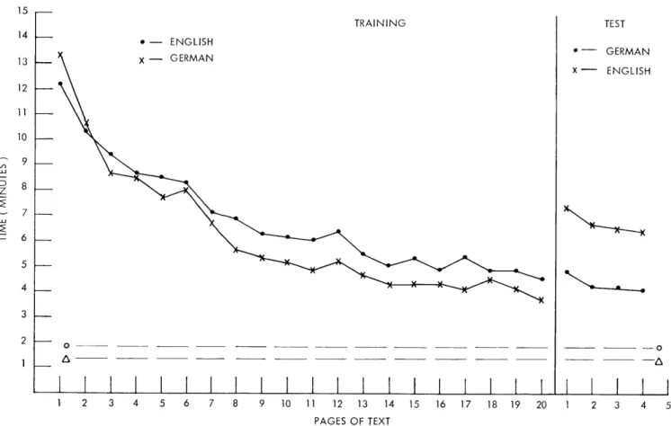
20 pages of German in inverted form, and then 4 pages of English. Also, on the first day, before reading any of the transformed text, and on the fourth day, after all of the transformations had been read, all of the subjects read 1 page of normal English and 1 page of normal German. The time taken by the subjects to read each page was meas-ured with a stop watch. The results are shown in Fig. XVII-1. The speed with which transformed English or German is read increases sharply with practice, from an initial

13 min/page to approximately 4 min/page. Even the latter rate, however, is consider-ably slower than that for normal text, while normal English (circles) takes a little longer than normal German (triangles). The transfer tests, however, produce asymmetrical results. The subjects trained on 20 pages of inverted English (closed circles)then read four pages of inverted German with no change in the level of performance; but the sub-jects trained on inverted German (crosses) did not do as well when tested on inverted English.

This work is supported in part by the National Science Foundation (Grant GP-2495), the National Institutes of Health (Grant MH-04737-04), and the National Aeronautics and Space Administration (Grant NsG-496); and through the Joint Services Electronics Pro-gram by the U. S. Army Research Office, Durham.

TRAINING * - ENGLISH X - GERMAN TEST *- GERMAN x - ENGLISH

I

li

l

I

I

Fig. XVII-1.

Results of transfer tests.

15 14 13 12 11 10 9 I-8 7 6 5 4 3 2 1 1 2 3 4 5 6 7 8 9 10 11 12 13 14 15 16 17 18 19 20 1 2 3 4 5 PAGES OF TEXT

(XVII. COGNITIVE INFORMATION PROCESSING)

This curious asymmetry of transfer has an analog in a number of sensori-motor coordinations, for which the general finding is that practicing the less favored organ per-mits more transfer to the more favored than the reverse direction does; for example, training a right-handed man's left hand on a complex task enables him thenceforward to perform the task with his right hand, but training his right hand does not usually enable him to perform the task with his left.2 In the present case we find that training in English enabled native speakers of German to transfer their skill without decrement, but training in German yielded some decrement for performance in English.

The more interesting aspect of these results has to do with what is learned when a subject learns how to decode transformed text. If he were learning only to recognize letters that had been transformed, transfer between the languages would be perfect, for the German and English alphabets are almost identical when Roman type is used, the only difference being the use of the diaresis, which does not affect letter shapes. If he were learning the shapes of words, transfer would be relatively poor, since German and Eng-lish word shapes are somewhat different. The results indicate that the learning cannot be as simple as either of these alternatives would have it.

P. A. Kolers, Ann C. Boyer

References

1. P. A. Kolers, M. Eden, and Ann Boyer, Reading as a perceptual skill, Quarterly Progress Report No. 74, Research Laboratory of Electronics, M. I. T., July 15, 1964, pp. 214-217.

2. _{R. S. Woodworth, Experimental Psychology (Henry Holt and Company, New York,} 1938).

B. PICTURE PROCESSING

1. OPTIMUM SCANNING DIRECTION IN TELEVISION TRANSMISSION

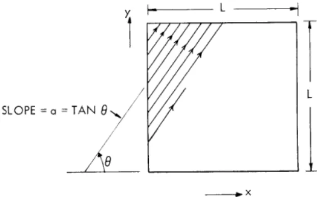
In television transmission, the two-dimensional picture is first scanned to produce a video signal which is then sent through some channel to the receiver. At the receiver, the picture is reconstructed from the video signal by scanning. For any given picture, different scanning methods usually give rise to different video signals and reconstructed pictures. In this report we shall discuss the relative merits of the members of a sub-class of scanning methods. We restrict our attention to constant-speed sequential scanning along equidistant parallel lines of slope a (Fig. XVII-2) and try to study the effect of scanning direction on the video signal and the reconstructed picture.

First, we shall find the direction of scanning (that is, the value of a) which yields the minimum-bandwidth video signal, assuming that the two-dimensional Fourier spec-trum of the original picture is given. Then we describe some preliminary results

(XVII. COGNITIVE INFORMATION PROCESSING)

Y L

SLOPE a = TAN 8L

X

-. x

Fig. XVII-2.

A subclass of scanning methods.

concerning the subjective effect of scanning direction.

Finally, we shall discuss some

miscellaneous factors that might affect the choice of a scanning direction.

Minimization of Video Signal Bandwidth

For the sake of simplicity, we shall assume in the following analysis that there is

no interlacing. Notice, however, that the addition of interlacing will not change the

result of the analysis.

Consider a single picture frame.

Let f(x,y) denote the brightness of the picture

point (with the average value substracted) as a function of its spatial coordinates (x, y),

under the assumption that f(x, y)

=

0 if (x, y) lies outside the picture.

Let 4 (T1, T

) be

the autocorrelation function of f(x,y); and #(u,v), the Fourier transform of

(71I,2),

that is, the energy spectrum of f(x,y).

Let

a

and

(w) be the autocorrelation

func-tion and the energy spectrum, respectively, of the video signal fa(t), derived from f(x, y)

by scanning along the direction a.

The question is: If #(u,v) is given, what value of

a will give the minimum bandwidth

a (w)? Without loss of generality, we assume that

the scanning speed is 1 unit length/unit time.

We also assume that the energy of the

picture signal is much larger than that of the synchronous and blanking pulses so that

the latter can be neglected.

Then, we have

4a(T)

T

-l1

where 0 = tan

a, assuming that both the distance between sucessive scanning lines

0)

In the case a - 0 or

o,

a(T)

of Eq. 1 gives only the central peak (at

=

0); however, the bandwidth of

a() is

deter-mined mainly by the central peak. In the sequel we shall assume that (1) is

an equality.

(XVII. COGNITIVE INFORMATION PROCESSING)

av, v) dv.

0

Assuming that 0

<--,

2

) _

+

a

a 2~ -. (+a2

w-av,

v)

dv.

Let us define the bandwidth of Da (w) as

f )

(w) dw

B

_a

-0

_#

a

₍₀₎

This definition is reasonable because a (c) - 0 for all o, and for most pictures, a (ce) have their maxima at w = 0. Now

I- 00

d a(w) d = 2rr a(0) = 2Tr (0, 0) (5'

is independent of a. So in order to minimize Ba, we have to maximize

4

a

2Tr

(-av, v) dv.

Hence, we want to choose that value of a which will maximize the right-hand side of Eq. 6. Referring to Fig. XVII-3, we have

SLOPE = a

SLOPE =- 1 /a

Fig. XVII-3. Pertaining to the interpretation of the right-hand side of Eq. 6.

(XVII. COGNITIVE INFORMATION PROCESSES)

+ a ) (-av, v) dv = 4(-z sin 0, z cos 0) dz. (7)

1

Notice that f(-z sin 0, z cos 0) is the value of f(u, v) along the straight line v =-- u which is perpendicular to the straight line v = au. To minimize Ba, therefore, we want to max-imize the right-hand side of (7), or equivalently, to maxmax-imize

f_

#(-z

sin 0, z cos 0)

dz

W (8)

W - (0, 0) (8)

2

1

We conclude, therefore, that in order to obtain the video signal of minimum band-width, one should scan the original picture along a direction perpendicular to the direc-tion of maximum bandwidth of '(u,v). This result is perhaps not in accord with one's intuition because, intuitively, one might think that to obtain the minimum-bandwidth video

signal, one should scan along the direction of minimum bandwidth of #(u,v); this is not the case according to our analysis.

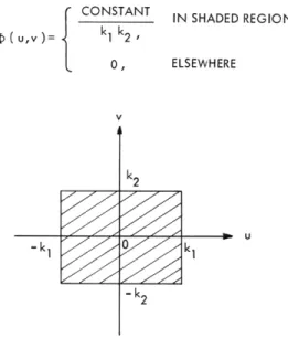
To verify the result of our analysis, we generated some two-dimensional lowpass Gaussian noise with power density spectra (Fig. XVII-4).

Constant _{for -k}

1 - u

<

<

(u, V) = (9)

0, elsewhere

where k1 and k2 are positive real constants. The results of this noise generation (with

DC level added) are shown in Fig. XVII-5. According to our analysis, to obtain the k

minimum-bandwidth video signal, we should scan along the directions k-. The appear-ance of the noise does seem to verify our contention.

We note in passing that if the scanning speed and the distance between successive scanning lines (which is assumed to be much smaller than L) are kept constant, then the scanning time per picture frame is independent of the direction of scanning.

Subjective Effect of Scanning Direction

At the ordinary viewing distance (4 or 6 times the picture height), one can see the line structures in the received picture. Do people prefer line structures of a particular orientation to those of other orientations ? To try to find an answer to this question, we generated pictures scanned along various directions on a closed-circuit television system. Some of these pictures are shown in Fig. XVII-6.

S( Uv)=

I

Fig. XVII-4.

Spectrum of two-dimensional lowpass Gaussian noise.

(a)

(b)

Fig. XVII-5.

_{Two-dimensional lowpass Gaussian noise. (a) kl/k}

2

= 1.

(b) kl/k

(XVII. COGNITIVE INFORMATION PROCESSING)

(a)

(b)

(c)

Fig. XVII-6.

Picture scanned along various directions.

preferences as follows.

Orders (in the order of decreasing preference): Subject A: Vertical, horizontal, skew. Subject B: Horizontal, skew, vertical. Subject C: Horizontal, vertical, skew. Subject D: Skew, horizontal, vertical. The preference, however, was by no means strong.

It is interesting to note that Subject C disliked skew scanning because it seemed to cause anxiety, while Subject D liked skew scanning because it made the picture look "dynamic." Subject B disliked vertical scanning because vertical lines seemed most

(XVII. COGNITIVE INFORMATION PROCESSING)

visible, and Subject D disliked vertical scanning because the picture seemed ready to fall apart.

Jumping to a tentative conclusion, we might say that the preference is not strong but horizontal scanning seems to have a slight lead.

Other Factors

The pictures mentioned in the preceding section are essentially noiseless. In prac-tice, however, the received picture contains additive random noise and ghosts (caused by multipath). _{How do the effects of random noise and ghosts depend on scanning} direc-tion? Also, how is motion affected by scanning direcdirec-tion? These questions are being investigated.

Finally, we wish to remark that there are still other factors that one might consider in choosing a scanning direction. For example,2 in skew scanning, the lines are not of equal length, therefore the power of the video signal does not have peaks at multiples of line frequency. Hence, when several video signals share the same channel, the use of skew scanning will reduce cross modulation. On the other hand, skew scanning com-plicates line synchronization.

T. S. Huang References

1. T. S. Huang, Two-dimensional power density spectrum of television random noise, Quarterly Progress Report No. 69, Research Laboratory of Electronics, M. I. T., April 15, 1963, p. 147.

2. Dr. B. Prasada, Bell Telephone Laboratories, Inc., Private communication, 1964.

2. BOUNDS ON TWO-ELEMENT-KIND IMPEDANCE FUNCTIONS

In a previous report, we discussed some bounds on the impedance functions of R, ±L, ±C, T networks. In this report, we shall present bounds for various types of two-element-kind impedance functions. We first prove a theorem for R, ±C and R, ±L net-works.

THEOREM 1. Let [Zik(s)] be an nth-order R,±C (or R, ±L) open-circuit impedance matrix. Then Zik(jw) satisfies

Zik(jw)-

_ik

₂

_ik

' i ii

2

kk''kk'"

for all real w.

The proof of Theorem 1 follows readily from the two following lemmas.

(XVII. COGNITIVE INFORMATION PROCESSING)

n

Zik(s)

h

(0) + h/s

h

+

h m)/(s+am

,

(2)

m=

1

where the real numbers am are independent of i and k, the

Lh

ij]

(r=

1,

2,.

,m;

0,

)

are real and symmetrical, and

F

) is positive semidefinite (psd)

ik j is negative semidefinite (nsd)

[h(m)

is

psd

if a

0, and nsdif a

<

0.

ik m m

LEMMA 2.

If [Pik] and [qik] (i, k= 1,2) are real, symmetrical, and psd, then

2p

q

< P

q

+

q

P

.

(3)

By making appropriate impedance transformations, we deduce from Theorem 1 two

theorems about ±R, C and ±R, L networks.

THEOREM 2.

Let [Zik(s)] be an n th-order ±R, C open-circuit impedance matrix.

Then Z ik(jw) satisfies

1 , 1

Zik(Jw)

(Zik(O)/jw + Zik()/jw)

-(Zii(O)/w

ii()/w)l

(Zkk()/w

Zk( )/w)

(4)

for any real w, where Z!k(s) = sZik(s).

THEOREM 3.

Let [Zik(s)] be an nth-order iR, L open-circuit impedance matrix.

Then Zik(jw) satisfies

Zik(jw) - - (jwZik(0) + jwZ ik(o))

(wZ"i (0) - wZ'. (0)) (WZIt (0) - WZ k(O))

(5)

for any real w, where Z!k (s)

=

Zik(s)/s.

Notice that inequalities (1),

(4), and (5) are properties of the impedance functions

and are independent of the manner in which one realizes these functions. When i k, the

inequalities give bounds on transfer functions; when i= k, they give bounds on

driving-point functions.

It is clear that for RC(RL) networks, both Theorem 1 and Theorem 2 (Theorem 3)

apply.

For any particular realization, N, of an RC n-port, the quantities in (1) and (4)

have the following physical interpretations:

Zik(0) = circuit impedance matrix of N, when all capacitances are

Z i()

= open-circuit impedance matrix of N, when all capacitances are

short-circuited

Z!k(0)/jw = open-circuit impedance matrix-of N, when all resistances are

short-circuited and s=jw

(XVII. COGNITIVE INFORMATION PROCESSING)

Zik(O)/jw circuit impedance matrix of N, when all resistances are open-circuited and s= jw.

(For any RL n-port realization, we have similar physical interpretations.) The quan-tities Z..(0), Z..(0), Z!'(0), and Z! (co) are not independent. In fact, we have the

fol-11 11 11 11

lowing lemmas.

LEMMA 3. Z. (0) is finite, if and only if Z!'(0) is zero.

11 11

LEMMA 4. Z. .(oo) is zero, if and only if Z! (oo) is finite.

11 11

In order to get useful bounds, one would like the right-hand sides of (1) and (4) to be finite. Hence, one would like to have Z. (ao) = 0 = Z! (0). One can achieve this by the

11 11

following procedure. Given an RC open-circuit impedance matrix [Zik(s)], we form a new RC open-circuit impedance matrix

[zik(s)] =

[Zik(s)]

Then z..(x) = 0 = z!.(0), where z!i(s) = sz. (s), and we can apply inequalities (1) and

11 11 11 11

(4) to zik(s) . For any nonzero finite w, the right-hand sides of (1) and (4) are finite,

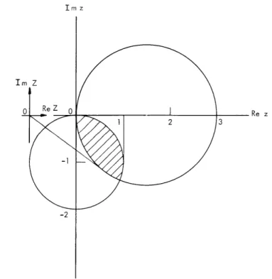
and zik(jw) must lie in the intersection of two nondegenerate closed circular disks.

Im z Im Z IM z

0

Re Z 0ii

Re z

(XVII. COGNITIVE INFORMATION PROCESSING)

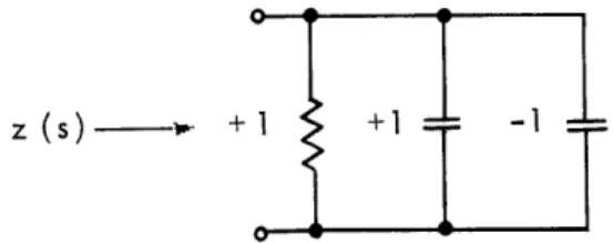
We conclude with an example.

Consider the RC driving-point impedance function

IZ(jw) - 5/21 < 3/2. Let Z'(s) = sZ(s). Then Z'(0) = 0 and Z'(oo) = ). Therefore, ine-quality (4), when applied to Z(s) directly, does not give any useful bounds. We can, how-ever, define z(s) = Z(s) - Z(co) - Z'(0)/s = 4(s+9/4)/(s+l)(s+3). Then z(0) = 3, z(o) = 0, z'(0) = 0, and z'()o) = 4. Hence for w= 2, say, Z(j2) must lie in the shaded region of Fig. XVII-7. In particular, we have

1 < IZ(j2) < 2.4, -370< [ Z Z(j2)]

<

<

Putting s = j2 in the exact expression for Z(s), we find Z(j2) = 2. 2/-33. 8.

In the previous report,1 we proved that if [Zik(s)] is the open-circuit impedance matrix of an R, ±L, ±C, T network, then

ik

2

(7)

where [Riko] is the open-circuit impedance matrix of the network when all reactive ele-ments are open-circuited, and [Riks] is the open-circuit impedance matrix of the network

z(s)--

+1

+

-1

Fig. XVII-8. Example of an R, ±C network.

when all reactive elements are short-circuited.

We remark that Eq. 1 does not follow from Eq. 7, since, in general, for an R, ±C network, Z. (0) # R ik and Z ik(o) R ik_{s .} For example, consider the network of

Ik

iko

ik

Iks

Fig. XVII-8. We have Z(s) = 1; therefore, Z(0) = 1 = Z(oo). But R = 1 and R = 0.

S

T. S. Huang

References

1. T. S. Huang and H. B. Lee, Bounds on impedance functions of R, ±L, ±C, T net-works, Quarterly Progress Report No. 75, Research Laboratory of Electronics, M. I. T., October 15, 1964, pp. 214-225.

(XVII. COGNITIVE INFORMATION PROCESSING)

C.

SENSORY AIDS

1. APPROXIMATE FORMULAS FOR THE INFORMATION TRANSMITTED BY A

DISCRETE COMMUNICATION CHANNEL

It is often desirable to have an approximate formula for the information transmitted

by a discrete communication channel which is simpler than the exact expression. I In

this report, two approximate expressions are derived. The derivations are instructive,

for they show why two systems that operate with the same probability of error can have

quite different information transmission capabilities.

Preliminary Theorems

The following theorems will be required.

The proofs of Theorem 1 and of the lemma

are omitted.

Theorem 2 follows directly from Theorem 1, and also from Fano's

dis-cussion.

THEOREM 1: Let xl, x2, ... , xn be non-negative real numbers. If F(x 1, 2,... ,x

)

xi , log

and if

n

xi

=

p,

then

F(p/n, p/n, .. ,p/n)

<

<

The equality sign on the left applies only if all the x's are equal. The equality sign on

the right applies only if all but one of the x's are zero.

THEOREM 2: Define

p(xi), probability of occurrence of the input xi to a communication channel,

p(yj), probability of occurrence of the output yj from a channel,

Lx, number of inputs having nonzero probability of occurrence, and

Ly, number of outputs having nonzero probability of occurrence.

Let

P(e lY) = 1 - p(xj yj).

(XVII. COGNITIVE INFORMATION PROCESSING

Ly

Ly

P(e) =

P -p(x

y )] p(yj) =

P(e y

p(y ).

j=1

j=1

If

H(elyj)

[P(e yj) log P(e yj) + [1 -P(elyj)

log [ - P(eyj)]]

Ly

H(e Y) I H(e yj) p(y),

j=1

and

H(e) = - P(e) log P(e) - (1- P(e)) log (1 -P(e)),

then

0 < H(e IY)

<

H(e).

LEMMA:

Let [p(y x)] be a conditional probability matrix having Lx rows and Ly

columns.

Consider the matrix [p(x y)], where

p(yj I xi) P(x

p(x

_j)

p(yj)

.th

If

Q.

denotes the number of nonzero off-diagonal terms in the

j

column of the matrix

.th

[p(y x)], then the number of nonzero off-diagonal terms in the j

row of the matrix

[p(x y)] is also

Q

.

Derivation of Upper and Lower Bounds for I(X; Y)

To derive the following bounds on I(X; Y) two different communication channels are

considered, each of which is required to transmit information about the same input

ensemble.

Both channels have the same number of outputs,

The two channel matrices

have identical elements on the main diagonal.

Therefore, P(e yI )

(j

= 1,2, ...

Ly) and

P(e) are the same for both channels.

One channel matrix has only one nonzero off-diagonal term in each column.

The

information transmitted by this channel is a maximum for fixed values of P(e y

The other channel has a matrix in which all nonzero off-diagonal terms in any one

column are equal. The information transmitted by this channel is a minimum for a given

number of nonzero off-diagonal terms in each column, and for fixed values of (Pe I j)

(j = 1, 2,

.

. . , Ly).

The information transmitted in this case is equal to the lower

bound in Eq. 3.

(XVII. COGNITIVE INFORMATION PROCESSING)

THEOREM 3: Let I(X; Y) be the information transmitted by a discrete channel, and Lx

H(X) = - p(xi) log P(xi).

i= 1

Let Qmax be the largest of Q1, Q'

''

Ly"

I(X; Y) < H(X)

-

H(e IY)

<

H(X);

I(X; Y) > H(X) H(e IY)

-j=1

Then

P(e IYj) p(yj) log Qj > H(X) - H(e) - P(e) log Qmax

PROOF:

p(i=

i= 1

j=1

p(x

yj)

P(xi IYj) P(Y ) log

p(x_{i )}

Ly

_Lx

= H(X) +

p(yj

i

j=1

i=

p(xi

) log p(x

yj) =

p(x

Iyj) log p(x

IYj)

Ly

I

P(Y )

(xj I

j=l

rj) log p(xj Iyj) +

p(x

_{IYj) log p(x}

i izj If we replace xi by p(xi y ), p by Lx

1-

i= 1

izj

[1 -p(xj

I Yj)] log

P(xi IYj)

and n by Qj, and if we use

p(x

yj) log p(xi

[1 -p(xj

yj)] log

[1

-p(xj yj )]

Qj

_<

i= 1

follow directly from Theorem 1 and the lemma.

The equality sign on the right applies if, and only if, there is only one nonzero off-diagonal term in the jth row of the p(x y) matrix. The equality sign on the left applies

(XVII. COGNITIVE INFORMATION PROCESSING)

if, and only if, all the nonzero off-diagonal terms in the jth row of the [p(x y)] matrix

are equal.

Substitution of the inequalities above in Eq. 1 results in

Ly

I(X; Y)

<

H(X) +

p(y.)

[p(x.

y) log

_{p(xj yj) + [1 -p(xj yj)] log [1 -p(xj y)]]}

j=1

<

H(X) - H(e IY).

(2)

Ly

[-

I(X; Y) > H(X) +

py

p(x y ) log p(x y

+

[1

-p(x

y)]

log

j=

1

Ly

> H(X) - H(e Y) -

P(ey) p(yj) log Qj.

(3)

j=1

Theorem 3 now follows from Theorem 2 and from the fact that

log Qmax

log Qj

(j = 1,2,

Ly).

Approximate Formula for I(X; Y)

In order to use upper and lower bounds to estimate I(X; Y) in such a way that the

expected value of the estimation error is minimized, it is necessary to know the

dis-tribution function for I(X; Y).

Since the distribution function is not usually available,

the estimate for I(X; Y) will be taken as the average of its upper and lower bounds. Such

an estimate minimizes the maximum possible estimation error.

It follows that we estimate that

Ly

II(X; Y) = H(X) - H(e Y) - ~ P(e yj) p(y) log

Qj

j=1

1

I (X; Y) = H(X) -~-(H(e)+ P(e) log Qmax) . (5)

The maximum estimation error e is given in each case by

Ly

e1

j= 1

1

(XVII. COGNITIVE INFORMATION PROCESSING)

The maximum error e in per cent, which results because the estimate for I was chosen midway between the upper and lower bound, is

e%= ( L 100%,

where U is the upper bound, and L is the lower bound. Thus

Ly

i

Q

j= 1

e

H(X) - H(e Y) -I P(e yj) p(y ) log Qj

j=1

1

-(H(e) + P(e) log Qmax)

e2 2 max 100o%. (9)

H(X) - H(e) - P(e) log

Qmax

The use of inequalities H(e Y) < H(e) and

Ly

SP(e

j=1

in (6) and (8) results in upper bounds for el and el%

e ~ P(e) log Qmax (10)

1

2max

1 P(e) log Q

el

2

max

100%,

(11)

H(X) - H(e) - P(e) log Qmax

which are easier to compute than the exact quantities given by Eqs. 6 and 8.

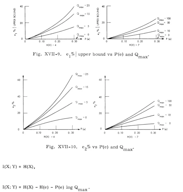
In Figs. XVII-9 andXVII-10 el% and e2% are plotted as functions of P(e) for various

values of

Qmax

for the cases H(X)

=

4 and H(X)

=

7.

It should be remembered

that these graphs represent the maximum errors that can occur as a result of

approximating I(X;Y) by I1(X; Y) and I2(X; Y).

The actual error that results when

I(X; Y) is approximated by 1

(X; Y) will equal the maximum error if and only

(XVII. COGNITIVE INFORMATION PROCESSING) Q =25 max z Q =15 D 0 5 max max 5 (3 = 0 0.10 0.20 0.30 H(X) = 4

Fig. XVII-9.

e

I

upper bound vs P(e) and

Q

max Q_max Q _max 5₅ Q -0 max - P (e) 0.10 0.20 0.30 H(X) = 4 max max Q max -- P(e) 0.10 0.20 0.30 H(X) : 7

Fig. XVII-10.

_{e2% vs P(e) and}

_Qmax

I(X; Y) = H(X),

₍₁₂₎

I(X; Y) = H(X) - H(e) - P(e) log Qmax (13)

Equation (12) holds if, and only if, all off-diagonal terms in the channel matrix are zero (a perfect communication system). Equation (13) applies if, and only if, H(e y ) = H(e), and

Qj

Similarly, the errors that result when I(X; Y) is approximated by Il (X; Y) are equal

to the maximum error only in special cases. If there is only one off-diagonal term in each column of the channel matrix, then

I(X; Y) = H(X) - H(e IY).

(XVII. COGNITIVE INFORMATION PROCESSING)

Ly

I(X; Y) = H(X) - H(e Y) - Z P(e ly) p(y.) log Qj.

j= 1

The estimate II(X; Y) is always better than or as good as I2(X; Y). However, the first estimate requires more computation than the latter. A useful procedure for esti-mating I(X; Y) is:

1. Evaluate e2 in per cent. If e2 is acceptable, evaluate I2(X; Y) as an

approxima-tion to I(X; Y).

2. If e2 is too large, evaluate the upper bound for e1 in per cent. If this upper bound

is acceptable, evaluate I1 (X; Y) as an approximation to I(X; Y).

3. If the upper bound to e₁ is too large, then compute I(X;Y) from the exact formula (1).

Example

The following channel matrix results when a human subject is required to make one of eight responses to one of eight equiprobable statistically independent stimuli. The information transmitted is to be computed to an accuracy of ±5 per cent of the true value.

Y1 Y2 y3 Y4 Y5 Y6 Y7 Y8 x1 .95 .05 x2 .05 .90 .05 x3 .05 .05 .90 x4 .10 .80 .10 = [P(ylx)]. x₅ .90 .05 .05 x6 .95 .05 x7 .05 .90 .05 x8 .05 .05 .90

Step 1: Computation of e2 (per cent)

max = 2

P(e) = 0. 10 H(X) = 3 e 2 = 11. 9%.2

(XVII. COGNITIVE INFORMATION PROCESSING)

The maximum error (per cent) resulting from the simpler estimate exceeds the desired ±5 per cent bound.

Step 2: Computation of e1 (per cent)

e 1< 2. 27o.

The maximum percentage in error that is caused by using I1(X; Y) as an estimate for I(X; Y) is within the required limits of accuracy.

8

2 P(e yj) p(yj) log Qj = 0. 050

j=

H(e IY) = 0. 383

1₁(X; Y) = 2. 57 bits/stimulus.

An exact calculation shows that I(X; Y) = 2. 59 bits/stimulus. Discussion

The amount of computation required for the estimate I1(X; Y) increases in proportion to the number of messages. The simpler estimate requires little computation and is independent of the number of messages. The maximum error (per cent) for both esti-mates decreases as H(X) increases, since the influence of H(e) in the denominator of equations (8) and (9) becomes less as H(X) becomes larger. When H(X) is small, the first estimate will usually be required. For larger values of H(X), the second estimate will usually yield acceptable values of e2 per cent. While it is true that the amount of

computation necessary for the evaluation of Il(X; Y) increases with the number of

mes-sages, it is also true that the probability that the simpler estimate will be satisfactory also increases with H(X).

R. W. Donaldson

References

1. R. M. Fano, Transmission of Information (The M. I. T. Press, Cambridge, Mass., and John Wiley and Sons, Inc., New York, 1961).