HAL Id: hal-00298340
https://hal.archives-ouvertes.fr/hal-00298340
Submitted on 3 Aug 2007
HAL is a multi-disciplinary open access
archive for the deposit and dissemination of
sci-entific research documents, whether they are
pub-lished or not. The documents may come from
teaching and research institutions in France or
abroad, or from public or private research centers.
L’archive ouverte pluridisciplinaire HAL, est
destinée au dépôt et à la diffusion de documents
scientifiques de niveau recherche, publiés ou non,
émanant des établissements d’enseignement et de
recherche français ou étrangers, des laboratoires
publics ou privés.
Variability of Antarctic intermediate Water properties
in the South Pacific Ocean
M. Tomczak
To cite this version:
M. Tomczak. Variability of Antarctic intermediate Water properties in the South Pacific Ocean.
Ocean Science, European Geosciences Union, 2007, 3 (3), pp.363-377. �hal-00298340�
Pacific Ocean
M. Tomczak
School of Chemistry, Physics and Earth Sciences, Flinders University, GPO Box 2100, Adelaide SA 5001, Australia Received: 29 September 2006 – Published in Ocean Sci. Discuss.: 1 December 2006
Revised: 22 February 2007 – Accepted: 10 July 2007 – Published: 3 August 2007
Abstract. Argo float time series data are used to study the
salinity field at the depth of the salinity minimum produced by Antarctic Intermediate Water (AAIW). It is found that far from showing the smooth erosion of the minimum that would result from diffusive flow, the salinity field is characterized by features of geostrophic turbulence such as fronts, eddies and intrusions. Comparison of the Argo float observations with the climatology of the World Ocean Atlas (WOA) re-veals significant differences between the two data sets. Some of the differences may have their origin in problems with the WOA data density in remote regions of the South Pacific, but most are more likely produced by interannual variations of the AAIW salinity field.
1 Introduction
The ocean is a fluid in turbulent motion. Turbulence creates eddies, meanders, filaments and fronts on a wide range of space and time scales and gives the fields of ocean currents and water mass properties intriguing texture.
In the upper ocean observational evidence of variability in time and textured structure in space has been available for considerable time. Information on the structure of the ocean below the permanent thermocline is much more limited, and maps of oceanic properties for the deep ocean usually give the impression that fields vary smoothly, in a manner more characteristic of slow diffusive flow than of a fluid filled with fronts and eddies.
The reason is of course the very low data density in the deeper ocean regions, which does not allow us to resolve the high spatial gradients associated with turbulent features. The landmark maps of the water masses of the Atlantic Ocean produced by W¨ust (1935) more than 70 years ago are
out-Correspondence to: M. Tomczak
standing historical examples; their smooth property fields, which were constructed from a total of some 250 observation points spread over the entire Atlantic Ocean, suggest uniform spreading of Antarctic Intermediate Water and Antarctic Bot-tom Water from the Southern Ocean towards the equator and smooth movement of North Atlantic Deep Water in the op-posite direction.
But even today’s much larger database is not sufficient to resolve the structure of the deep ocean in enough de-tail. The World Ocean Database and associated World Ocean Atlas (Ocean Climate Laboratory, 2002), the most compre-hensive data set for studying the deep ocean and available online from many oceanographic research institutions, pro-duces high quality decadal mean property distributions but cannot reveal the high degree of space and time variability that does without doubt exist. To this day observational data only allow occasional confirmation of the existence of turbu-lent features such as isolated eddies at great depth (Armi and Zenk, 1984; McWilliams, 1985; Elliot and Sanford, 1986; Prater and Sanford, 1994; Tomczak and Andrews, 1997).
The situation is likely to change with the introduction of the Argo float programme. Argo floats are drifting platforms for the measurement of temperature and salinity as functions of depth over periods of years (Roemmich et al., 2004). They can be programmed individually for specific tasks; but a typ-ical Argo float follows one of two operational modes. In the simple mode, the float drifts at a certain depth, often 2000 m, rises to the surface every 10 days to take a temperature and salinity profile from that depth, stays at the surface for up to 12 h to transmit the data via satellite, and returns to its deep drifting depth. In the park and profile mode, the float is parked at a certain depth (the Argo operations centre recom-mends 1000 m), descends to 2000 m every 10 days to start the temperature and salinity profile, comes to the surface, trans-mits its data and returns to its parking depth. In the beginning of 2006, 46% of floats profile to around 2000m and 66% pro-file to depths greater than 1500 m.
364 M. Tomczak: South Pacific Antarctic intermediate Water variability
While Argo float deployments use a parking depth too shallow to allow insight into space and time variability of Deep and Bottom Water, most Argo floats dive deep enough to traverse the Antarctic Intermediate Water (AAIW) as part of their regular profiling pattern. This makes it possible to extract information on the degree of spatial AAIW variabil-ity. This paper uses Argo float data obtained until mid-2005 to investigate the structure of the AAIW salinity field in the South Pacific Ocean.
2 Data and methods
The drift of an Argo float is determined by three factors: the ocean current at its parking depth, the surface current dur-ing the 6–12 h period while the float transmits its data, and the current profile during ascent and descent. The relative contributions of each factor to the overall drift are difficult to determine. Ichikawa et al. (2001) estimate that the drift at the parking depth is overestimated by 10–25% as a result of effects of current shear during ascent and descent and uncer-tainties from the determination of the exact location where the float surfaces (which may happen some time before a satellite passes and picks up the signal). A very basic esti-mate of the surface and parking depth contributions to the overall drift can be obtained by assuming that surface cur-rents are an order of magnitude larger than curcur-rents at 1000– 2000 m depth. This corresponds roughly to the ratio of the time when the float drifts at its parking depth to the time of measurement and data transmission, suggesting that surface and parking depth drift contribute about equally to the overall drift.
The hypothesis underlying the present study is that Argo floats will stay in the same water parcel while drifting at parking depth but will be moved away from that water par-cel when they traverse the upper ocean and follow the sur-face current; as a result they will encounter a different parcel of water every time they return to their parking depth. In a study of Antarctic Intermediate Water this assumption is obviously better met by floats that park at 1000 m than at 2000 m depth. It is also closer to reality in the centres of the subtropical gyres, where the permanent thermocline is depressed and AAIW is found at or below 1000 m, than in the tropics where the thermocline rises and AAIW is found closer to 500 m.
Whatever the particular circumstances of individual floats may be, it is fair to assume that any change of water proper-ties observed at the depth of AAIW is due to the fact that the float encountered different parcels of AAIW after every as-cent and dive cycle. This allows us to study the spatial struc-ture of AAIW in some detail. AAIW is particularly suited to such a study because it is associated with a distinct salin-ity minimum. If the ocean is dominated by smooth diffusive flow, any change in the salinity minimum observed by the floats should be slow and uniform, from lower salinity
val-ues closer to the AAIW formation region to higher valval-ues further afield. If, on the other hand, the flow is turbulent and AAIW is interspersed with fronts and eddies, variations of the AAIW salinity minimum will show more random be-haviour.
Having formulated our hypothesis we now investigate the suitability of the available data for the purpose of the study. The Argo float data set comprised all floats available for the Pacific Ocean between 52◦S and 10◦N on the Argo database in June, 2005. The data were individually inspected for data errors and sensor drift. Occasional erroneous data (data that fell clearly outside any physically reasonable salinity range) were eliminated while the remaining profile was retained. Where an entire salinity profile fell outside any reasonable temperature-salinity (TS-) relationship the profile was elim-inated while the remaining profiles of the float in question were retained.
To investigate AAIW variability, time series of the AAIW salinity minimum were constructed by extracting the salinity minimum from the depth range 500–1200 m of every float profile. (The lower limit of 1200 m was set by the lowest profiling depth of the majority of floats, the upper limit by the shallowest depth of the AAIW salinity minimum in the tropics.) With a typical sampling interval of 50 m in and be-low the permanent thermocline Argo floats do not necessarily resolve the minimum salinity if it falls between two observa-tion levels. Cubic spline interpolaobserva-tion to 10 m intervals was used to improve the resolution.
To obtain a reference time series representative of smooth diffusive evolution of the salinity minimum, the AAIW salin-ity minimum along the track of each float was reconstructed from the World Ocean Atlas (WOA; Conkright et al., 2002). The WOA data were assigned to the centre of their respective 1◦square for this purpose, and the salinity profile along the float track was determined by spatial linear interpolation of the annual mean WOA field. Temporal interpolation using seasonal WOA data was not considered appropriate, the as-sumption being that the AAIW seen by the float was water that moved more or less with the float and was out of reach of the seasonal changes that operate during the AAIW for-mation process.
The standard deviation of the resulting salinity minimum time series can serve as a measure of the variability caused by the movement of the float through the climatological mean field. It can be compared with the standard deviation of the salinity minimum time series obtained from the Argo float, and the ratio between the two can serve as an indicator of the departure from slow diffusive flow.
The extraction of a salinity minimum time series repre-sentative of AAIW relies on the existence of an interme-diate salinity minimum between 500 m and 1200 m depth. Some floats occasionally generated profiles that reached be-low 500 m depth but did not extend deep enough to capture the salinity minimum. Such profiles were accepted if their total number was small compared to the length of the time
Fig. 1. Launch locations of Argo floats used in this study. Here and in the following figures the “coastline” represents the 1000 m contour.
series and if the salinity at the deepest level was very close to the minimum salinity found in the remainder of the pro-files; the salinity at the deepest level was used as the salinity minimum in these cases. Other floats generated profiles with no intermediate minimum in the entire 500 m–1200 m depth range. (This occurred particularly when a float drifted too far south into the region where the salinity minimum comes closer to the surface.) Such profiles were excluded from the analysis.
Several floats showed obvious sensor drift or calibration problems. No attempt was made to recalibrate dubious pro-files. Any attempt to correct profiles by bringing them closer to values obtained during previous profiles or to existing cli-matologies would reduce the variability that is the focus of this study and produce a bias towards low variability. It was therefore essential to base the study on real-time quality-controlled data and not on delayed-mode quality quality-controlled data.
The maximum Argo depth of 2000 m is also not deep enough to use the properties measured at that depth as time and space invariant anchor points. A practical way of reject-ing floats with drift problems was found by inspection of the standard deviations. Severe drift increases the standard de-viation of the time series dramatically, and by rejecting all floats with a standard deviation of the salinity minimum time series of 0.06 or more all obviously erroneous floats were eliminated. This still leaves floats that display some drift but of a magnitude comparable to true signals. These floats have to be inspected individually and are discussed in some detail in a later section.
171 Argo floats passed the detailed data quality review and form the basis of the study. Figure 1 shows their launch loca-tions. While the float density in the centre of the subtropical gyre is low, much of the region is covered well. The 171 floats provided 9515 profiles. The shortest float track con-tained 4 profiles, the longest 179. About 40 floats produced more than 40 profiles, most contributed between 60 and 90 profiles. 11 floats contributed more than 90 profiles each.
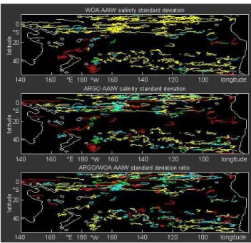
Fig. 2. Argo float trajectories colour-coded to show the variabil-ity of the AAIW salinvariabil-ity minimum. Top panel: Standard devi-ation (stdev) of the AAIW salinity minimum time series derived from the WOA data along the float tracks. Colours are defined by yellow: stdev<0.0075; cyan: 0.0075<stdev<0.0125; green: 0.0125<stdev<0.0175; red: stdev>0.0175. Middle panel: as top panel but stdev derived from the Argo float data. Bottom panel: ratio of the standard deviation from the Argo float data to the stan-dard deviation from the WOA data. Colours are defined as yellow: ratio<2; cyan: 2<ratio<4; green: 4<ratio<6; red: ratio>6.
3 Results
Figure 2 shows three versions of the 171 float trajectories. The trajectories in the top and middle panel are colour-coded according to the magnitude of the standard deviation of their AAIW salinity minimum time series. The time series in the top panel are derived from the WOA salinity field, in the mid-dle panel from the Argo float observations. Smallest standard deviations are indicated by yellow, larger standard deviations by cyan and green; largest standard deviations by red.
Features to note are the large regions of very low standard deviations, particularly in the WOA-derived time series, the strongly elevated standard deviations between Australia and the date line and west of Peru, and the generally larger stan-dard deviations in the Argo-derived time series. To demon-strate the latter finding, the bottom panel shows the ratio of the standard deviations.
It appears evident from the figure that AAIW variability in the ocean is larger than what can be expected from slow diffusive flow. To give an estimate of the scale on which the observed variability is occurring, Fig. 3 shows a histogram of the distance between successive float surfacing locations. Most floats travel some 10–40 km between successive data transmissions, but there is also a considerable range of larger
366 M. Tomczak: South Pacific Antarctic intermediate Water variability
Fig. 3. Histogram of distances (km) between successive surfacing locations of the Argo floats used in this study.
distances. Very large distances are produced by data trans-mission failures causing gaps in the time series. Assuming that about half the float movement is caused by drift at the surface and the other half by drift at the parking depth, the standard deviations of Fig. 2 indicate the degree of variabil-ity on space scales varying from 5 km to about 100 km and more.
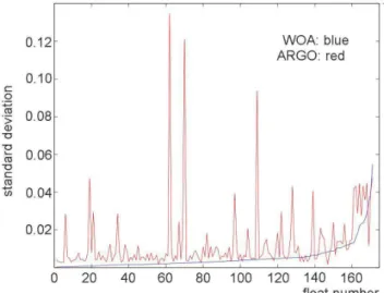
Figure 4 investigates the magnitude of the AAIW variabil-ity found in the Argo float observations in more detail. In this figure the 171 floats are sorted according to the standard de-viation of their associated WOA-based time series. While the WOA-derived time series show a slow increase of the stan-dard deviations from near-zero to about 0.005 for the first 140 floats followed by a rapid increase to 0.03, the Argo-derived standard deviations are more uniform and closer to 0.006 before following the steep rise and show several par-ticularly large values. It should be noted that values below 0.003 are below the resolution of the salinity algorithm. The low values for the WOA-derived time series are the result of floats passing through a highly smoothed salinity field. Most Argo-derived values, on the other hand, are clearly larger than the sensor resolution and do not represent mere instru-mental noise. The Argo team guarantees an accuracy of 0.01 for delayed mode quality controlled data, despite the fact that the instrument stability is often closer to 0.003 (Wijffels, per-sonal communication), but Oka (2005) estimates sensor drift at as low as 0.004 per year, based on recalibration of recov-ered floats. About half the floats used here have a standard deviation less than or close to the accepted accuracy if the larger Argo accuracy of 0.01 is used as a yardstick.
Fig. 4. Comparison of standard deviation of the AAIW salinity min-imum from the WOA-derived time series and from the time series derived from the Argo floats. The floats are sorted by the WOA-derived standard deviation, which therefore represents a monotonic series (the blue line). The red curve shows the corresponding float-derived standard deviation.
4 Discussion
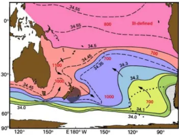
Before we address the AAIW variability seen in the Argo floats in detail it is necessary to understand the features of the underlying climatological mean field seen in the WOA data. AAIW in the South Pacific Ocean is supplied from two different sources with slightly different minimum salini-ties (Tomczak and Godfrey, 2003). The two AAIW variesalini-ties meet in the New Zealand region, which leads to water move-ment at 700–1100 m depth across strong salinity gradients (Fig. 5) in the western South Pacific.
In contrast, the eastern South Pacific is characterized by the spreading of a single AAIW variety from its formation region near southern Chile to the tropics. In the south this creates a strong meridional salinity minimum gradient and a “shadow zone” in the tropics, where the salinity minimum is not always well defined.
Another reason for elevated standard deviations in the WOA-derived time series could be the data distribution in the World Ocean Data Base (WOD01: Conkright et al., 2001). Salinity data are far less numerous than temperature data. Large differences in the number of observations in neigh-bouring cells, or different bias towards different seasons, can potentially lead to differently weighted means that can result in unrealistic salinity gradients. Strong seasonal affects at the depth of AAIW are unlikely, but data density decreases rapidly with depth, and means from sparse data can produce distortions of the field.
To identify possible effects of varying data density the WOA data distribution for the 1000 m depth level in the South Pacific was investigated. Figure 6 shows some
Fig. 5. Long-term mean distribution of salinity at the depth of the AAIW salinity minimum. The depth of the minimum is also in-dicated; light shading indicates regions where the minimum is at the surface. The dotted line in the southeast marks a region where surface salinities are lower than those shown for the minimum at 700 m. East of New Zealand the water depth is too shallow for In-termediate Water to occur. Adapted from Tomczak and Godfrey (2003).
essential statistics. As can clearly be seen, the South Pacific Ocean, particularly its eastern region, is one of the least ex-plored regions of the world ocean. South of 20◦S from the date line to 90◦W it is possible to identify individual research expeditions in the data distribution. Standard deviations are generally higher in regions of higher data density, but the cor-respondence is not followed throughout; in the Tasman Sea the highest data density is found along the Australian shelf, while the largest standard deviation is located north of New Zealand, suggesting that the meeting zone of the two AAIW varieties is a region of increased spatial and temporal vari-ability.
The World Ocean Atlas applies a weighted average over an area of influence around each grid cell to smooth the data fields. Figure 6c demonstrates the sparseness of the data in the South Pacific Ocean: In large regions south of 20◦S, but also in isolated meridional strips in the tropics, the salinity field at the 1000 m depth level is determined by very few observations.
Turning now to the observations obtained by the Argo floats, it appears useful to structure the discussion by dis-tinguishing a number of possible processes that influence AAIW variability. The 171 time series can be grouped in five categories: smooth quasi-diffusive flow, elevated variability, interannual change in the large-scale salinity field, fronts and eddies, and multiple salinity minima. Each of these cate-gories will now be addressed in turn.
Fig. 6. Data distribution in the WOA data set at the 1000 m depth level. (a) number of observations per one degree square, (b) stan-dard deviation where there is more than one data point in a one degree square, (c) number of “points of influence” used in the cal-culation of the field.
4.1 Smooth, quasi-diffusive flow
The time series in this category are represented by the floats with standard deviations close to the base level of the red curve in Fig. 4 (values close to 0.006) and a low standard de-viation ratio. They represent the majority of all 171 floats. However, it is premature to conclude that at the depth of AAIW the ocean is not in a turbulent state. It may simply mean that at spatial resolution of 5–50 km the elements of turbulence do not have a large imprint. Even stations that follow the climatological mean closely have a standard de-viation well above instrument noise level, indicating that the salinity field does have texture on these scales (Fig. 7). This texture is likely to be the product of some turbulent cascade, as will become more evident when the other categories are considered.
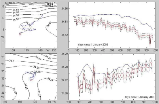
Float 5900324 spent 900 days in a region of very low salin-ity gradients just north of the Equator. Towards the end of the time series it entered a region of lower salinity in the north, crossing a moderate gradient in the process. The AAIW salinity minimum recorded by the float shows a similar trend to the AAIW salinity minimum derived from the WOA data
368 M. Tomczak: South Pacific Antarctic intermediate Water variability
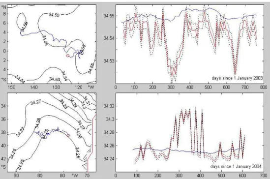
Fig. 7. Time series of the AAIW salinity minimum for Argo floats 5900324 (top) and 3900121 (bottom). The left panels show the float trajectories superimposed on the AAIW salinity minimum field derived from the World Ocean Atlas; the red circle indicates the start of the drift. Contours are drawn at 0.01 intervals. The smooth (blue) curves in the right panels are the time series of the AAIW salinity minimum along the float track derived from the Atlas. The red curves are the Argo float observations. The dashed lines indicate the instrumental resolution (±0.003). The Argo team gives 0.01 as salinity accuracy, slightly more than three times the indicated range.
Fig. 8. As Fig. 7 but for Argo float 3900120.
and a short term variability that barely exceeds the instrument resolution.
Float 3900121 spent 700 days in the low salinity region of the subtropical eastern South Pacific. An initial westward excursion during the first 100 days was followed by a return to the original launching region. Based on the WOA data this should have resulted in a rise and fall of the AAIW salinity minimum during the first 150 days. The Argo observations show several short-lived events of higher AAIW salinity dur-ing that period, which is dominated by AAIW salinities be-low 34.27. Agreement between the WOA field and the float observations is reached after the first 250 days. This suggests that in 2004 the region of AAIW salinities <34.27 reached
further west than indicated by the WOA field and that it was bounded by a rather sharp gradient, which was encountered by the float on several occasions during the first 150 days of its life.
Many floats that show a low standard deviation ratio dis-play a significant difference between the AAIW salinity min-imum observed at the floats and the AAIW salinity minmin-imum along the float track derived from WOA. At first sight this could suggest a calibration problem. This may occasionally be the case for individual floats but is less likely for entire float neighbourhoods that show the same difference. Such a situation is more likely an indicator for interannual changes in the AAIW salinity field, which are further discussed in
Fig. 9. As Fig. 7 but for Argo floats 39047 (top) and 4900334 (bottom).
Sect. 4.3. In the situation shown in Fig. 8, for example, the float record suggests that the mean salinity field was shifted some 10◦towards west. There is also some indication of reg-ular east-west movement of the salinity field, indicated by the brief periods of higher AAIW minimum salinity, although the two year long record is not long enough to establish this with any certainty.
4.2 Elevated variability
While variations in the AAIW salinity minimum can exceed the instrument resolution occasionally in floats of Sect. 4.1 (in the example of Fig. 8 they exceed it by a factor of 2–3), float records in Sect. 4.2 show variations that are significantly larger than the instrument resolution. Figure 9 shows two examples.
Float 39047 represents one of the longest float trajecto-ries of the 171 floats studied. It spent more than five years in the centre of the subtropical gyre. During the first three years of its life the AAIW properties experienced by the float were very different from the AAIW properties of the WOA field. The fact that from day 1300 onward both AAIW prop-erties show excellent agreement suggests very strongly that the float retained its calibration through the entire five year period. The reasons for the departure of the observed AAIW salinity minimum from the WOA field are difficult to estab-lish. It could be an indication of a large scale shift of the mean field, but it could also indicate uncertainty in the WOA field itself; the data distribution on which the WOA field is based has some significant holes in the region (Fig. 6). The Argo team assessed float 39047 as corrupted (Wijffels,
per-sonal communication). The argument is discussed in more detail in the Appendix. In the present context the float serves to demonstrate the possible validity and significance of ele-vated standard deviations.
Float 4900334, a shorter record from the equatorial region, presents an example of a different situation that leads to ele-vated standard deviation. Its time series mirrors the general shape of the corresponding WOA field but “exaggerates” its gradients. Sparsity of WOA data is not a problem in this re-gion, and the difference between the time series is most likely an indicator of the extent at which the WOA smoothing pro-cedure weakens actual spatial gradients.
4.3 Interannual change in the large-scale salinity field Some Argo time series mirror the WOA field closely but are shifted in location. This does not produce a large difference in standard deviation (in other words, these stations are also part of the cohort in Fig. 4 that shows values close to 0.006) but indicates significant interannual variations in the loca-tion of the major features of the climatological mean field. The shape of the isotherms of Fig. 5 may remain unchanged, but the entire field will have shifted. Individual Argo floats are insufficient to resolve whether the observed shift of the mean field is an expression of large-scale geostrophic turbu-lence, possibly the low wave number end of the cascade for which the high wave number end is seen in the time series of Sect. 4.1.
Figure 10 shows the time series of two floats from the high gradient region to the north east of New Zealand. The two floats spent their lives in similar mean field gradients but in
370 M. Tomczak: South Pacific Antarctic intermediate Water variability
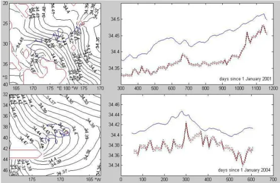
Fig. 10. As Fig. 7 but for Argo floats 5900105 (top) and 5900443 (bottom). Ocean regions shallower than 1000 m are delineated in red.
Fig. 11. As Fig. 10 but for Argo float 5900360.
locations separated by 1600 km in space. They belong to dif-ferent release batches, and their launching dates were several hundred days apart. Both floats show a discrepancy between the WOA field and the float observations of the same mag-nitude that is sustained throughout the observation period. It can also be seen that in both cases the float time series can be made to match the AAIW salinity minimum of the WOA mean field if they are shifted to higher salinities and slightly back in time. This can be interpreted in a number of ways, some more convincing than others.
That the salinity sensor calibration of a large number of floats might contain the same erroneous offset is highly un-likely. Shifting the time series to higher salinities is equiva-lent to shifting the float trajectories westward relative to the WOA mean field. Systematic errors in the positioning sys-tem of many floats are also highly unlikely. The conclusion has to be that the WOA mean field places the salinity gradient region to the west of the situation observed in 2003–2005.
The floats did not spend their lives in a data-sparse region (compare Fig. 6), and there is no reason to think that the AAIW salinity field given by the World Ocean Atlas should not be accepted as representative of the long term mean situ-ation north east of New Zealand. This suggests that Antarc-tic Intermediate Water that reached the area was about 0.03– 0.06 less saline during the years 2001–2005 than the clima-tological average. One possible explanation can be found in the time difference between the Argo data and the WOA. All data of WOA 2001 were taken before the first Argo float was deployed in the region, and the bulk of the WOA 2001 data stems from earlier decades. Wong et al. (1999) found a freshening of AAIW in South Pacific transects along 32◦S
of 0.03–0.06 over a time span of twenty years, comparable to the difference found here between the Argo data and WOA 2001.
The calculation of the WOA time series along the track is based on the annual mean. It has been suggested that
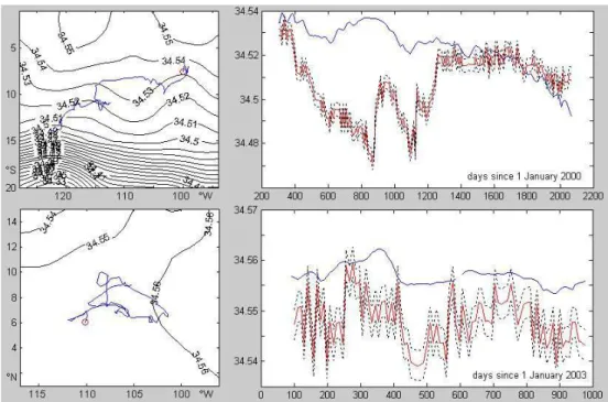
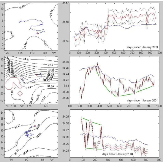
Fig. 12. As Fig. 10 but for Argo floats 3900103 (top), 5900097 (centre) and 3900225 (bottom). Green lines highlight the presumed evolution of separate AAIW varieties.
the observed differences between WOA and Argo could be an indication of climatological seasonality of the salinity field. The available data are too sparse to verify this. In-spection of the seasonal WOA salinity fields for the region at 1000 m depth reveals differences between seasons of up to 0.08 (i.e. larger than the observed differences between WOA and Argo); but inspection of the data density shows that most seasonal mean fields were constructed from one or two cruises that traversed the region in different directions during different years and left large areas without any data coverage. It is therefore by no means clear whether the dif-ferences between seasons in the WOA data set represent sea-sonal or interannual variability.
A different but also similar situation is seen further north in the sub-equatorial region (Fig. 11). Here the AAIW salin-ity minimum recorded by the float shows very good agree-ment with the WOA mean field, particularly if the float time series is shifted forward by 50–100 days. Since the float moved eastward, a forward shift in time corresponds to an
eastward shift relative to the mean field, or a westward shift of the mean field. Although this is not a data-rich region for the World Ocean Atlas its data density is still acceptable, and it appears that the observed shift is more likely the effect of interannual movement of the salinity field than a bias in the climatological mean field itself.
4.4 Fronts and eddies
Many Argo time series contain sudden large changes in the AAIW salinity minimum time series that can indicate the crossing of a front. The evidence is not very conclusive if it occurs only once and is not much larger than the underly-ing salinity variability, but there are stations where the time series clearly indicates repeated crossings of the same front. Such repeated crossings can occur if the track of the float is strongly influenced by the surface current, which reversed during the observation period, bringing the float back into a previously visited AAIW parcel. They can also indicate a convoluted frontal shape that leads to repeated crossings
372 M. Tomczak: South Pacific Antarctic intermediate Water variability
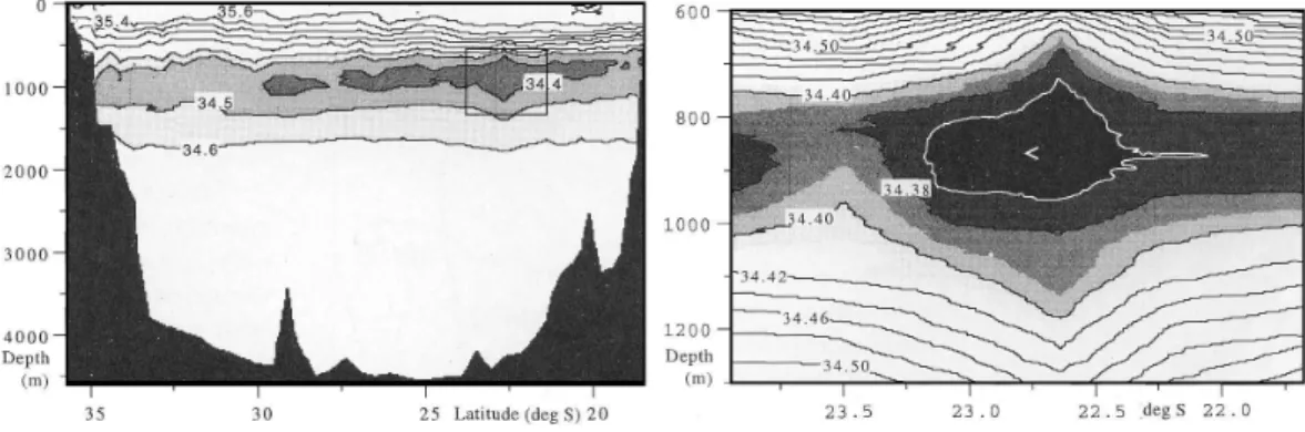
Fig. 13. A submerged eddy in the depth range of Antarctic Intermediate Water observed in section P14C of the World Ocean Circulation Experiment (WOCE) across the South Fiji Basin. The right panel is an enlargement of the rectangle indicated in the left panel. Adapted from Tomczak and Andrews (1997).
along a straight float track. The figures that follow can only give a few examples of the many situations of sudden large variations in the AAIW salinity minimum.
Float 3900103 (Fig. 12 top) spent nearly three years in the equatorial region where the AAIW salinity minimum is weakly defined and gradients are extremely small. Its salinity record generally agrees well with WOA climatology, but the salinity field still contains frontal structures at a very large distance from the source of the salinity minimum: Around day 400 the float clearly crossed from a region characterized by a minimum salinity of 35.555 to a region where the salin-ity minimum is closer to 35.563. The change is just large enough to fall outside instrumental detection limits and oc-curs at a point where the WOA climatology indicates an in-crease in the minimum salinity as well.
Float 5900097 (Fig. 12 centre) spent nearly three years in a region with a very large salinity gradient. Throughout its life it experienced sudden changes of up to 0.06 in the minimum salinity at AAIW level. It might be tempting to suspect in-strumental instability or temporary fouling of the conductiv-ity cell; but inspection of the temperature-salinconductiv-ity (TS-) dia-gram for the float (not shown) verifies that the cell performed without problems and that the float encountered two varieties of AAIW with different salinity minimum values. The TS-diagram gives additional support for the presence of a front between the two varieties by showing that profiles taken near the transition between the two varieties often display double salinity minima indicative of layering and intrusions across the front. The discussion of Sect. 4.5 will address double minima in more detail.
Float 3900225 (Fig. 12 bottom) presents a case where the float was initially located over a well established front but moved away from it after about 160 days, when its record begins to mirror the smoothness of the climatological field. While it was near the frontal region it found its parking po-sition sometimes on the high salinity side of the front, some-times on the low salinity side. If the mean of the two salini-ties is taken it corresponds well to the climatological mean.
A frontal crossing associated with a salinity increase (de-crease) followed by a frontal crossing associated with a salin-ity decrease (increase) can be produced by an eddy. Tomczak and Andrews (1997) reported an AAIW eddy between New Zealand and Fiji. The eddy had its core at 900 m and did not extend into the surface layer. It was associated with a salinity difference of 0.2 with its surroundings and measured some 100 km across (Fig. 13). An Argo float with a typical sur-face position separation of 20 km corresponding to a spatial resolution at AAIW depth of 10 km would see this eddy as an elevated salinity minimum at 10 successive profiles, after which the profile would return to the values recorded before the eddy was encountered. A longer lasting influence can be expected if the eddy moves with the current at AAIW depth, which is likely to be close to the current experienced by the float at parking depth.
Situations that can be interpreted as eddy crossings have been observed. Figure 14 shows two examples. The tropical trajectory of float 5900208 followed more or less the climato-logical 34.55 isohaline but experienced two instances where the AAIW salinity minimum dropped below 34.525. Salini-ties as low as that are not found anywhere near the location of the float. The most likely explanation for the observed episodes are passages of bodies of AAIW that could main-tain its original low salinity longer than usual. Dynamically this is usually achieved through rotation; in other words, the isolated body of low salinity AAIW is transported as an eddy. The second example shown in Fig. 14, float 3900222, spent nearly two years in the low salinity region off the south-ern west coast of Chile, the formation region of the low salinity AAIW variety that dominates the eastern South Pa-cific (Fig. 5). During most of the time the AAIW proper-ties recorded by the float agreed well with the climatologi-cal mean. But for a period of some 120 days it encountered a variety of AAIW with significantly higher salinity. The records suggests that the boundary between the two varieties had the character of a well defined front: The salinity record switches back and forth between salinities around 34.25 and
Fig. 14. As Fig. 10 but for Argo floats 5900208 (top) and 3900222 (bottom).
34.31, indicating that the float parked itself on different sides of the front.
4.5 Multiple salinity minima
Some of the observed large standard deviations in the Argo float data are produced by the occasional presence of double salinity minima. The minimum-seeking routine is not capa-ble of tracking individual minima but always selects the low-est salinity in the 500 m–1200 m depth range. Where double minima change their strength along the track of a float, the routine can select different minima for different profiles and create the appearance of large sudden salinity changes not unlike those observed at fronts.
Double minima suggest that the formation of intrusions and filaments that leads to layering within a water mass are part of the turbulence at AAIW level. Multiple intrusions have been reported on several occasions from the region around New Zealand, where two varieties of AAIW with identical densities establish a front (Stanton, 2002; Tomczak and Godfrey, 2003). The results of this study suggest that their occurrence may be more widespread than previously known.
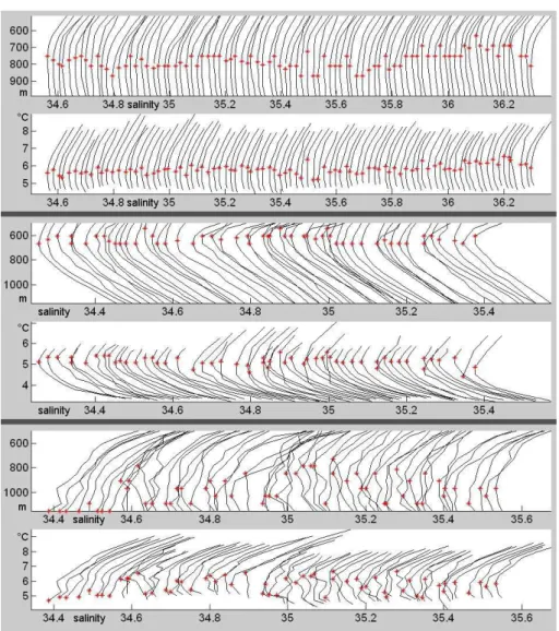
Figure 15 shows “waterfall plots” of salinity-depth profiles and TS-diagrams of three selected floats for the depth range dominated by AAIW. Float 5900324, already discussed in the context of Fig. 7, is representative of a smooth salinity field where the variability barely exceeds the instrumental resolution. When its data are displayed in a waterfall plot the salinity-depth profiles and TS-diagrams appear as a sequence of evenly spaced, nearly identical curves.
Float 3900222, already discussed with Fig. 14, represents a situation dominated by strong frontal crossings. In the wa-terfall plots they appear as gaps between groups of closely clustered salinity-depth profiles. The corresponding TS-diagrams all display the shape typical for the AAIW salinity minimum, but the magnitude of the minimum changes when a front is crossed, which makes the TS-diagram sequence gappy, too.
Float 5900443 demonstrates the effect of double minima. Because the minimum detection routine does not detect mul-tiple minima the time history of the float, already seen in Fig. 10, does not reveal their existence but gives the impres-sion that a somewhat elevated variability is superimposed on the climatological mean. It is also noticeable that not every profile exhibits multiple minima. If only a single minimum is present it is sometimes found at the lower end of the depth range reached by the float (particularly at the beginning of the record), which makes the result of the minimum detec-tion routine quesdetec-tionable. Such situadetec-tions were generally ex-cluded from the analysis but are retained here to demonstrate the variability typical for the region east of New Zealand, where the AAIW salinity minimum is found at depths below 1000 m. The intermittent occurrence of multiple minima in-dicates that the associated layering and intrusions occur on relatively small spatial scales, smaller than the scales asso-ciated with fronts such as those seen in the record of float 3900222.
374 M. Tomczak: South Pacific Antarctic intermediate Water variability
Fig. 15. Salinity against depth and temperature (TS-diagram) for Argo floats 5900324 (top), 3900222 (centre) and 5900443 (bottom). The salinity scale is valid for the first curve on the left; successive curves are shifted by 0.02. Red marks indicate the salinity minimum identified by the minimum detection software.
5 Conclusion and outlook
The salinity minimum produced by the spreading of Antarc-tic Intermediate Water provides a unique opportunity to use Argo float data for a test of the turbulent character of deep ocean currents. The investigation presented here shows be-yond doubt that eddies, fronts, intrusions and filaments are a regular feature of the water mass structure at the depth of the AAIW salinity minimum and that the water masses do not spread in a diffusive but in a turbulent field.
It is of course of interest whether turbulence occurs uni-formly across the ocean or whether it is concentrated in a few limited regions. To gain some insight into this ques-tion the horizontal salinity gradient at the depth of the AAIW salinity minimum was calculated between successive surfac-ing locations. In most situations a large gradient indicates the presence of a front. Occasionally it is the produced by the presence of multiple minima.
In Fig. 16 all 171 float tracks are shown by their succes-sive surfacing locations, marked by the magnitude of the ob-served horizontal salinity gradient. A preferred region of large gradients cannot be made out; large gradients are found in all regions of the South Pacific. A distinct tendency for fewer large gradients in the tropics should not be taken as an indication for reduced turbulence in the equatorial current system, where currents are known to be particularly strong and thus prone to turbulence. Most likely the low number of large gradients in the tropics is a consequence of the weak-ness of the AAIW salinity minimum in that region, which makes it difficult to produce large gradients even in fronts. The existence of fronts in the tropics was already shown with float 3900103 (Fig. 12 top), but the salinity change across the front is so small that it does not register under the criteria of Fig. 16.
Fig. 16. Argo float surfacing locations colour-coded to show the occurrence of large horizontal gradients in the AAIW salinity minimum. A green dot indicates a gradient dS/dl<0.001 km−1, a blue asterisk a gradient 0.001 km−1≥dS/dl≥0.002 km−1, a red asterisk a gradient
dS/dl≥0.002 km−1.
The analysis leaves many questions. As the number of floats and the length of their time series increase it should be possible to subdivide the float ensemble into individual years, map the salinity field for the depth of the AAIW salin-ity minimum and compare it with the climatological mean of the World Ocean Atlas. This would give insight into the de-gree of interannual variability. Where groups of floats were released in close vicinity it may be possible to map the size of individual eddies they encounter.
There is no reason to believe that the character of the prop-erty fields in water masses other than AAIW differs substan-tially from the turbulent character of the AAIW salinity field. The unique situation of AAIW, which can so easily be iden-tified through its salinity minimum, makes its analysis par-ticularly easy. Other water masses require more sophisti-cated methods of analysis, for example analysis on density surfaces. The main impediment to an extension of the analy-sis to the water masses of the deep ocean is the limited depth coverage of Argo floats. As time goes on, more floats will reach to at least 2000 m depth, which will give access to the upper reaches of Deep Water.
Appendix A
The data quality of float 39047
Float 39047 spent its life in the tropical eastern Pacific Ocean, moving slowly westward from 7◦S 100◦W to 14◦S
123◦W, covering the distance of more than 2600 km in just
under 5 years. After an initial period of three months, when its data followed the WOA climatology closely, its TS-data departed significantly from the WOA climatology for 2.5 years before returning to climatology during the second half of its history (from July 2003; Fig. 9, day 1300). The Argo team assessed its data quality as affected by sensor fouling and based this assessment on a comparison of its
TS-Fig. A1. The water masses of the thermocline of the Pacific Ocean. PCW: Pacific Central Water, PEW: Pacific Equatorial Water, S: South, N: North, W: Western, E; Eastern. Adapted from Tomczak and Godfrey (2003). The red line indicates the approximate track of float 39047, the black line WOCE section P18.
data with climatology and neighbouring floats, not only at the AAIW level but across the permanent thermocline as well (Wijffels, personal communication).
TS-relationships of thermocline water masses are well de-fined and very tight, so comparison of data on the basis of
376 M. Tomczak: South Pacific Antarctic intermediate Water variability
Fig. A2. Cumulative TS-diagram for WOCE section P18 between the Equator and 30◦S (black) and Argo float 39047 (red). The shift from high to low salinity at temperatures above 10◦C indicates the transition from Equatorial and Central Water to subpolar water. The black line through the data is the TS-diagram of the WOCE P18 sta-tion at 15◦S in the centre of the frontal zone between subtropical and subpolar water masses. The data show the presence of the Tran-sition Region at the section in 1994.
thermocline TS-relationships is usually a good tool for qual-ity control. The thermocline of the Pacific Ocean contains several varieties of Central and Equatorial Water, each con-fined to its own region and separated by neighbouring va-rieties by well defined fronts, which complicates their use as a quality control tool. Two extensive “transition zones” between Central and Equatorial Water and subpolar water masses are found along the eastern periphery (Fig. A1).
The eastern South Pacific is among the least explored re-gions of the world ocean, and the location of the water mass boundaries is not well established. Based on the schematic sketch offered by Tomczak and Godfrey (2003) WOCE sec-tion P18 along 103◦W should have been in South Pacific Equatorial Water to about 20◦S and in East Pacific Cen-tral Water until about 30◦S, where it should have entered the “Transition Zone” and begin to show lower salinities in-dicating subpolar influences. Inspection of data from the section indicates that when the section was performed in 1994 the transition region reached significantly further west; lower thermocline salinities were observed well before 30◦S
(Fig. A2). When the TS-data of Argo float 39047 are com-pared with the WOCE section it is seen that the float data are inside the envelope of the WOCE P18 TS-data, suggesting that all data from the float represent oceanic properties from the region and should therefore be acceptable in principle.
Comparison with neighbouring floats is less conclusive. Several floats (3900062, 3900067, 3900118) are either cor-rupted from the start or show severe drift. Other floats (3900159, 3900108), which agree with the WOA
climatol-ogy, were not deployed until mid-2003 when the TS-record of 39047 also began to return to climatology. Float 39053, which began recording in early 2001 some 650 km north west of float 39047, returned only four values over a pe-riod of a few months that show much variability (if they can be trusted). Float 39032, which began recording in October 2000, returned only eight values over a period of months that match the WOA climatology well but fall into the early ob-servation period of 39047, when its data also matched the climatology.
Float 3900066, the nearest float of comparable quality, was launched in late 2001 some 1650 km south east of 39047, well within the Transition Zone. It shows similarly large TS-variability, and its TS-data overlap with those of 39047.
If the observations from float 39047 are accepted as cor-rect they would indicate significant interannual variability in the location of the boundary between South Pacific Equato-rial Water and the Transition Zone and suggest an extensive westward shift of the boundary during the first 2.7 years of observations from the float. The years 2002 and 2003 wit-nessed one of the strongest El Ni˜no episodes in history, and it is tempting to speculate that the apparent widening of the Transition Zone off South America might be related to that episode.
A relocation of water mass boundaries of hundreds of kilo-meters from the surface to more than 1000 m depth is a ma-jor event, and more evidence is required to verify that it oc-curred during 2002–2003. All available evidence suggests, however, that the data recorded by float 39047 during that period cannot be dismissed lightly and probably recorded a true event.
Acknowledgements. I thank L. A. Barlow for the preparation of
the float data and production of the first statistics and S. Wijffels for comments and suggestions. Comments from two reviewers and from the editor improved the clarity of the paper.
Edited by: T. Suga
References
Armi, L. and Zenk, W.: Large lenses of highly saline Mediterranean water. J. Phys. Oceanogr., 14, 1560–1576, 1984.
Conkright, M. E., Locarnini, R. A., Garcia, H. E., O’Brien, T. D., Boyer, T. P., Stephens, C., and Antonov, J. I.: World Ocean At-las 2001: Objective Analyses, Data Statistics, and Figures, CD-ROM Documentation, National Oceanographic Data Center, Sil-ver Spring, MD, 17 pp., 2001.
Conkright, M. E., Antonov, J. I., Baranova, O., Boyer, T. P., Gar-cia, H. E., Gelfeld, R., Johnson, D., Locarnini, R. A., Murphy, P. P., O’Brien, T. D., Smolyar, I., and Stephens, C.: World Ocean Database 2001, Volume 1: Introduction, edited by: Levitus, S., NOAA AtlasNESDIS 42, U.S. Government Printing Office, Washington, D.C., 167 pp., 2002.
Oka, E.: Long-term sensor drift found in recovered Argo profiling floats, J. Oceanogr., 61, 775–781, 2005.
Prater, M. D. and Sanford, T. B.: A meddy off Cape St. Vincent. Part I: Description, J. Phys. Oceanogr., 24, 1572–1586, 1994. Roemmich, D., Riser, S., Davis, R., and Desaubies, Y.:
Au-tonomous profiling floats: Workhorse for broadscale ocean ob-servations, Mar. Techn. Soc. J., 38(1), 31–39, 2004.
ening of the intermediate waters in the Pacific and Indian Oceans, Nature, 400, 440–443, 1999.
W¨ust, G.: Schichtung und Zirkulation des Atlantischen Ozeans. Das Bodenwasser und die Stratosph¨are, Wiss. Ergebn. Dt. Atl. Exp. “METEOR” 1925–1927, Berlin, 6, 1–288 (translated as “The stratosphere of the Atlantic Ocean” by Emery, W. J. (1978)), Amerind, 1936.