Radiative effects of secondary ice enhancement in coastal Antarctic clouds

HAL Id: insu-02042380

https://hal-insu.archives-ouvertes.fr/insu-02042380

Submitted on 4 Mar 2021

HAL is a multi-disciplinary open access

archive for the deposit and dissemination of

sci-entific research documents, whether they are

pub-lished or not. The documents may come from

teaching and research institutions in France or

abroad, or from public or private research centers.

L’archive ouverte pluridisciplinaire HAL, est

destinée au dépôt et à la diffusion de documents

scientifiques de niveau recherche, publiés ou non,

émanant des établissements d’enseignement et de

recherche français ou étrangers, des laboratoires

publics ou privés.

Gillian Young, T. Lachlan-Cope, S. J. O’Shea, C. Dearden, Constantino

Listowski, K. N. Bower, T. W. Choularton, M. W. Gallagher

To cite this version:

Gillian Young, T. Lachlan-Cope, S. J. O’Shea, C. Dearden, Constantino Listowski, et al..

Radia-tive effects of secondary ice enhancement in coastal Antarctic clouds. Geophysical Research Letters,

American Geophysical Union, 2019, 46 (4), pp.2312-2321. �10.1029/2018GL080551�. �insu-02042380�

Radiative Effects of Secondary Ice Enhancement in

Coastal Antarctic Clouds

G. Young1 _{, T. Lachlan-Cope}1_{, S. J. O'Shea}2 _{, C. Dearden}3_{, C. Listowski}4 _{, K. N. Bower}2 _,

T. W. Choularton2 _{, and M. W. Gallagher}2

1_{British Antarctic Survey, NERC, Cambridge, UK,}2_{School of Earth and Environmental Sciences, University of} Manchester, Manchester, UK,3Centre of Excellence for Modelling the Atmosphere and Climate, School of Earth and Environment, University of Leeds, Leeds, UK,4_{LATMOS/IPSL, UVSQ Université; Paris-Saclay, UPMC Univ. Paris 06} Sorbonne Université, CNRS, Guyancourt, France

Abstract

Secondary ice production (SIP) commonly occurs in coastal Antarctic stratocumulus, affecting their ice number concentrations (Nice) and radiative properties. However, SIP is poorly understood and crudely parametrized in models. By evaluating how well SIP is captured in a cloud-resolving model, with a high-resolution nest within a parent domain, we test how an improved comparison with aircraft observations affects the modeled cloud radiative properties. Under the

assumption that primary ice is suitably represented by the model, we must enhance SIP by up to an order of magnitude to simulate observed Nice. Over the nest, a surface warming trend accompanied the SIP increase; however, this trend was not captured by the parent domain over the same region. Our results suggest that the radiative properties of microphysical features resolved in high-resolution nested domains may not be captured by coarser domains, with implications for large-scale radiative balance studies over the Antarctic continent.

Plain Language Summary

Climate models do not always represent clouds well—particularly in Antarctica—because we do not fully understand them on a small scale. Clouds can affect the

temperature of the surface by reflecting energy from the Sun or trapping in heat from below; therefore, they play a crucial role in Antarctica, where warming surfaces are affecting how the ice shelves are melting. We need a variety of measurements of Antarctic clouds to understand them, including how many droplets or ice crystals they contain. Using measurements from the “Microphysics of Antarctic Clouds” project, we found evidence that, at certain temperatures, significantly more ice particles can be rapidly produced when fragile ice crystals or freezing droplets break up. We use these measurements to improve how cloud ice crystals are simulated in a weather model and consider implications for the frozen surface as a result of these changes. We found better agreement with our measurements by making the ice crystals multiply more efficiently in the model. As a result, less cloud cover was simulated and more energy from the Sun reached the surface, suggesting that the Antarctic surface may be subject to more warming than we originally thought.

1. Introduction

Cloud feedbacks represent the largest source of variability and uncertainty in radiative predictions by the global circulation models (GCMs) used within the Coupled Model Intercomparison Project (Dufresne & Bony, 2008). In particular, global model biases in absorbed shortwave (SW) radiation due to interactions with clouds are at their largest over the Southern Ocean (Bodas-Salcedo et al., 2012; Hyder et al., 2018; Kay et al., 2016).

Numerical models across spatial scales often underestimate Southern Ocean and coastal Antarctic cloud fractions with comparison to satellite observations (Bodas-Salcedo et al., 2014), leading to SW biases at the surface (Hyder et al., 2018; Vancoppenolle et al., 2011) which can hinder skilful forecasts of the sea ice extent. Low, widespread clouds dominate in this region during the summer months (McCoy et al., 2014) which can strongly influence radiative interactions (Klein & Hartmann, 1993). With too little low-level cloud modeled, not enough SW radiation is reflected, leading to enhanced surface warming.

RESEARCH LETTER

10.1029/2018GL080551

Key Points:

• Increasing modeled secondary ice production (SIP) by 10 times improves agreement with ice number concentration observations in Antarctica

• Enhanced SIP reduces cloud fraction and increases amount of shortwave radiation reaching the surface over a high-resolution nested domain • SIP-induced changes in cloud

radiative forcing over the

high-resolution nest are not captured by the coarse parent domain

Supporting Information: • Supporting Information S1 Correspondence to: G. Young, [email protected] Citation: Young, G., Lachlan-Cope, T., O'Shea, S. J., Dearden, C., Listowski, C., Bower, K. N., et al. (2019). Radiative effects of secondary ice enhancement in coastal Antarctic clouds. Geophysical

Research Letters, 46, 2312–2321. https://doi.org/10.1029/2018GL080551

Received 19 SEP 2018 Accepted 1 FEB 2019

Accepted article online 19 FEB 2019 Published online 25 FEB 2019

©2019. American Geophysical Union. All Rights Reserved.

Observations of these low stratus clouds have shown that they are moderately supercooled (between −21 and 0◦C; Grosvenor et al., 2012) and are typically mixed-phase yet are often dominated by supercooled liquid drops (Lachlan-Cope et al., 2016; O'Shea et al., 2017). Ice number concentrations, Nice, are typi-cally low given the moderate supercooling (often<0.07 L−1_{; Grosvenor et al., 2012) and ice nucleating} particle (INP) number concentrations predicted using the DeMott et al. (2010) parametrization overes-timate Nice. However, Listowski and Lachlan-Cope (2017) demonstrated that the DeMott et al. (2010) parametrization still compared better with in-cloud ice measurements over the Antarctic Peninsula than tra-ditional ice number concentration parametrizations (e.g., Cooper, 1986; Meyers et al., 1992) used widely in cloud-resolving models.

While these clouds are dominated by liquid droplets, isolated patches of high Niceoccur (Grosvenor et al., 2012; O'Shea et al., 2017): concentrations which have been attributed to secondary ice production (SIP). SIP is poorly understood and can occur via numerous mechanisms. Fundamentally, SIP involves the break up or multiplication of ice crystals formed through primary nucleation processes (Field et al., 2017). The warm supercooled temperatures accompanying these high N_icemeasurements in Antarctic clouds are often associated with the rime-splintering, or Hallett-Mossop (H-M), mechanism (Hallett & Mossop, 1974). Rime splintering is an efficient SIP process, where splinters grow from rime accreted on an ice particle through collisions with cloud droplets or raindrops. The fragile rime coating breaks easily, producing numerous daughter particles and enhancing the Nice. Occurring between −8 and −3◦C, H-M is typically diagnosed from the presence of high number concentrations (tens to hundreds per liter) and columnar ice crystals (Mossop, 1985a).

Our poor understanding of SIP leads to crude representations of these processes in numerical models. H-M rime splintering is often parametrized using the temperature-dependent triangle function detailed by Reisner et al. (1998). However, this parametrization lags behind current theories of H-M SIP, as observa-tional evidence suggests that this process is also dependent on the cloud droplet distribution and cloud type (Hobbs & Rangno, 1998; Mossop, 1985b; Mossop & Hallett, 1974).

SIP has the potential to affect cloud microphysical structure and radiative properties from the high Nice pro-duced and subsequent interactions with the cloud liquid phase through the Wegener-Bergeron-Findeisen (WBF) mechanism. To better understand the role of SIP in coastal Antarctic clouds, the Microphysics of Antarctic Clouds (MAC) aircraft campaign was conducted in the austral summer of 2015, from 21 Novem-ber to 14 DecemNovem-ber, sampling aerosol particle, cloud, and boundary layer (BL) properties over the Weddell Sea. Data have been summarized previously by O'Shea et al. (2017). Where ice was observed at temperatures spanning the H-M range, the number concentrations were enhanced by up to three orders of magnitude with respect to predicted INP concentrations (O'Shea et al., 2017).

Here we evaluate how well SIP is captured in a numerical weather prediction model—the polar-optimized Weather Research and Forecasting (PolarWRF; Hines & Bromwich, 2017; Skamarock & Klemp, 2008) model—using our MAC aircraft observations for comparison and adapt the H-M parametrization to improve agreement with our measurements. Specifically, we focus on the modeled Nicedistribution and consider how it affects cloud radiative forcing (CRF); forcing which is crucial for accurately predicting the evolution of Antarctic surface temperatures in a warming climate.

2. Methods

2.1. Instrumentation and Model

We concentrate on two flights from the MAC campaign to test our ability to model H-M SIP. Flights M218 and M219 were performed on the same day (27 November 2015) and in the same region, within a low pres-sure system over the eastern Weddell Sea (Figure 1a). Therefore, we combine these observations into one case study.

The Meteorological Airborne Science INstrumentation used aboard the British Antarctic Survey's Twin Otter research aircraft during the MAC campaign has been detailed previously (O'Shea et al., 2017). Ice particle measurements from the 2-Dimensional Stereo (2-DS) particle imaging probe (SPEC Inc., Lawson et al., 2006) are used for comparison with the PolarWRF model. As an optical array shadow probe, the 2-DS images particles of (nominal) sizes from 10 to 1,280𝜇m and can only skilfully conduct phase separation in mixed-phase clouds at particle sizes>80 𝜇m; therefore, we exclusively compare between obser-vations and model data in this size range. Anti-shatter tips were fitted to the 2-DS, and all particles with an

Geophysical Research Letters

10.1029/2018GL080551

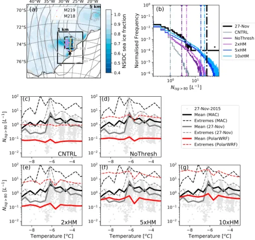
Figure 1. (a) Parent and nest domain structure. Flight tracks shown for M218 (orange) and M219 (purple). Dashed

black line outlines subset of the nest used for direct comparison with the aircraft data. NSIDC daily sea ice fraction (shading) and ERA-Interim (Dee et al., 2011) mean sea level pressure at 1800 UTC on 27 November 2015 (gray contours, hPa) overlaid. No sea ice data are available in the gray-shaded regions close to the coast. (b) Normalized frequency distribution of total ice number concentrations greater than 80_𝜇m (N_{isg> 80}) for our case study observations and the five model simulations. Data are binned in 0.2 L−1intervals, from which a frequency distribution is

constructed. Extreme values of each distribution are also shown (dot-dashed vertical line). (c–g) Nisg> 80as a function of temperature for the case study observations (gray), total MAC campaign (black), and PolarWRF (red). Solid line: mean; dashed line: extreme values (mean+3_𝜎). All observations from the 27 November case study are shown in light gray. Data are binned in 0.5◦C intervals for calculating statistics. (c) CNTRL; (d) NoThresh; (e) 2×HM; (f) 5×HM; (g) 10×HM. Model data taken below 1,500 m only. NSIDC = National Snow and Ice Data Centre; MAC = Microphysics of Antarctic Clouds; PolarWRF = polar-optimized Weather Research and Forecasting.

interarrival time< 1×10−6_{s were rejected to reduce the probability of measuring shattered particles. Further} details on observational data are included in supporting information S1 (Baumgardner et al., 2001; Glen & Brooks, 2013).

SW and longwave radiation were modeled using the Rapid Radiative Transfer Model for GCMs. The Mor-rison cloud microphysics scheme (MorMor-rison et al., 2005, hereafter, M05) was used within version 3.6.1 of the PolarWRF model: M05 has been previously shown to perform well in reproducing Antarctic clouds by reducing biases in both the cloud supercooled liquid water and the associated surface radiative fluxes in simulations over the eastern Antarctic Peninsula (Listowski & Lachlan-Cope, 2017).

M05 simulates single-moment liquid—with a prescribed droplet number averaged from the two case studies (92 cm−3_{)—and double-moment ice, snow, graupel, and rain. Here summed ice, snow, and graupel} num-ber concentrations>80 𝜇m (Nisg>80) were compared with the measured Niceby the 2-DS. Average aerosol particle number concentrations measured during the two flights by a GRIMM 1.109 portable aerosol spec-trometer, between sizes 0.5 and 1.6𝜇m (0.49 scm−3_{), were used as input to the DeMott et al. (2010) primary} ice nucleation parametrization in the M05 scheme.

SIP is represented by the H-M mechanism (Hallett & Mossop, 1974) in the M05 microphysics scheme. A SIP-enhanced ice crystal number concentration is produced by multiplying an empirically derived splin-ter production rate—350 splinsplin-ters per milligram of rime accreted (Pruppacher & Klett, 1997; Reisner et al., 1998)—by the mass production rate of rime on a snow(graupel) particle and a temperature-dependent multiplication factor.

PolarWRF model options are detailed in supporting information S1 (Bigg, 1953; Bromwich et al., 2013; Chen et al., 2018; Dearden et al., 2016; Nakanishi & Niino, 2006; Prein et al., 2015). The model was run for 48 hr, to allow adequate time for spin up, at high spatial resolution. We used two domains: a parent domain of 201 × 201 grid points with 5-km grid size and a nest of 326 × 406 grid points with 1-km grid size (Figure 1a). Seventy vertical𝜂 levels were used up to a model lid of 50 hPa, arranged to provide 25 levels within the lower 2 km of the domain (similar to Stevens et al., 2018). A 30-s time step was used in the parent domain, nested to a 6-s time step over the inner domain. We test how well the model is performing in close spatial vicinity to the measurements by considering a subset of the 1-km nested domain, indicated in Figure 1a.

2.2. Experiment Design

SIP onset in the M05 scheme is restricted by three thresholds: (1) snow mass mixing ratios must be≥0.1 g/kg; (2) cloud liquid water mixing ratio≥0.5 g/kg or rain water mixing ratio ≥0.1 g/kg; and (3) there must be a nonzero rimed mass on snow or graupel particles. Threshold (2) provides high liquid thresholds that are likely unattainable by these mixed-phase stratocumulus (see supporting information S1).

We conducted five model simulations to evaluate how well observed SIP is captured: (1) control (CNTRL), with no changes; (2) liquid thresholds for SIP removed (NoThresh); (3) 2× multiplication factor due to H-M mechanism with no liquid thresholds (2×HM); (4) 5×HM; and (5) 10×HM.

3. Results

3.1. Comparison With Measurements

Niceoccurs in patches during both flights, in agreement with the average findings of the campaign (O'Shea et al., 2017). Modeled clouds were predominantly liquid, with high Nisg>80occurring in isolated patches

(Figure S8), in agreement with our observations. Modeled ice patches within the BL often, although not exclusively, coincided with the presence of ice above the BL or updraughts at the BL temperature inversion, suggesting that seeding from above is a potential cause for the formation of BL ice patches (see supporting information S1).

Observed SIP occurs on short spatial and temporal scales against a low background of primary Nice; there-fore, SIP episodes will be extreme values of the Nicedistribution. We use these statistical extremes—values at the mean+3𝜎 (99.7%) level—to investigate SIP in the modeled clouds and are henceforth labeled as “extreme values.” We use 2-DS number concentrations greater than 0.005 L−1_{as an indicator for an observed ice} patch, and smaller concentrations were excluded when calculating mean values for comparison between measurements and the model.

Figure 1b shows the frequency distribution of 2-DS measured Niceand modeled Nisg>80for the five considered

simulations. At observed Nice >8 L−1, there are only a few occurrences for each measurement. Modeled Nisg> 80in the CNTRL produces a frequency distribution in poor agreement with the 2-DS observations.

Reducing the onset thresholds of the H-M parametrization increases the magnitude of the extreme values and improves the shape of the Nisg>80distribution. Both the distribution shape and extreme values improve

significantly by increasing H-M, with best agreement again found with the 10×HM simulation.

Figures 1c–1g show all 2-DS Nicedata from our case study as a function of temperature (gray), in addition to the mean and extreme values. Maximum Nicemeasured was 87.3 L−1during the 27 November case study, skewing the mean and extreme values at approximately −6◦C. Data from all stratocumulus clouds mea-sured during the full campaign are included for context (black) to infer where our case study may have poor measurement statistics.

The 27 November case study provides similar trends with comparison to the mean and extreme values cal-culated from all MAC data above −6◦C. However, the case study lacks good measurement statistics below −6◦C, and the whole MAC data set illustrates that high Niceare observed in this limit. MAC extreme values are approximately one order of magnitude greater than those calculated from the case study at temperatures

Geophysical Research Letters

10.1029/2018GL080551

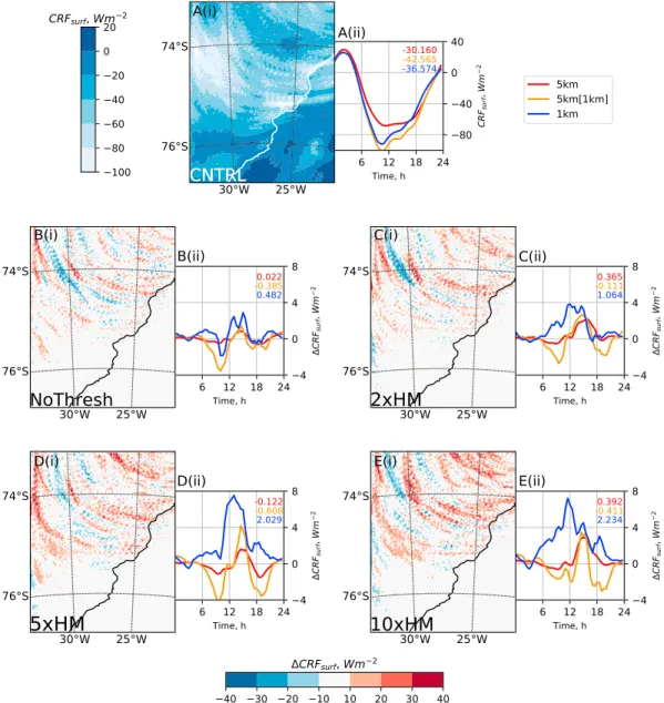
Figure 2. (a(i)) Map of day-averaged cloud radiative forcing at the surface (CRFsurf) over the 1-km nest; (a(ii)) time series of CRF_surf, with the day average of each domain configuration quoted in the top right corner. 5 km (1 km) refers to the area of the 5-km domain spanning the 1-km nested region. Figure structure is the same for (b)–(e), except anomalies with respect to the CNTRL (a) are shown. (b) NoThresh, (c) 2×HM, (d) 5×HM, and (e) 10×HM.

below and above −6◦C. However, agreement is good at −6◦C, suggesting that the high N_icemeasurement during the case study is skewing the whole data set.

From Figure 1c, the mean and extreme values from the CNTRL compare poorly with observations. Extreme value agreement significantly improves by removing the liquid thresholds on the H-M mechanism (Figure 1d, NoThresh). This improvement continues when increasing the H-M multiplication factor by 2, 5, or 10 times (Figures 1e–1g). While the absolute magnitudes of the mean modeled N_{isg> 80}become more comparable with the observations, the observed Nicetrends across the temperature range are not suitably reproduced. For example, the sharp peak at −6◦C is not captured by any simulation, and the mean Nisg> 80

are all too low greater than −6◦C. Despite this, the extreme values of the 10×HM distribution compare best with those of the full MAC data set above approximately −8◦C.

These comparisons indicate that the modeled cloud microphysical structure is more representative of our case study (and likely the whole MAC data set) when the H-M mechanism is efficient, with no liquid thresholds, and has a magnitude of 10× that typically used in cloud-resolving models.

3.2. Cloud Radiative Effects

While improving agreement with our observations, increasing H-M by 2, 5, or 10 times significantly increases the modeled N_{isg> 80}. Given this increase, the cloud macrophysical properties are likely affected by the microphysical effect of the WBF mechanism, thus influencing the radiative balance at the surface. To assess radiative implications of increasing H-M, we consider an adapted formula for CRF at the surface (CRFsurf), detailed in supporting information S1 (Ramanathan et al., 1989; Vavrus, 2006), which excludes reflected SW radiation from the calculation and combines the net longwave with downwelling SW at the surface. This adapted formula isolates SW differences due to changes in cloud cover from interactions with the high albedo surface. Figure 2 shows maps of day-averaged CRF_surf, where quoted mean CRF_surfvalues illustrate how much the surface is warmed or cooled with respect to clear skies.

In the CNTRL (Figure 2a(i)), modeled cloud cover is clearly affected by the low pressure system shown in Figure 1a. Time series of these data (Figure 2a(ii)) indicate greater coverage of these liquid-dominated clouds (Figure S8) in the 5-km domain over the nested area (labeled 5-km [1-km]), as indicated by a lower CRFsurf, than in the high-resolution nest. These results suggest that the WBF mechanism is better resolved in the 1-km domain, causing more cloud liquid depletion. However, over the whole parent domain, there is less cloud cover (cooling the surface less) than in the nested area, suggesting that the nested area may not be representative of the larger region.

Figures 2b–2e show anomalies (ΔCRFsurf) of our four adapted H-M runs with respect to the CNTRL. In panel (i) of each, red (blue) indicates more (less) SW radiation is reaching the surface than in the CNTRL, indicating less (more) liquid-dominated cloud cover is present. With increasing H-M, more SW reaches the surface. This warming effect is not uniform across the nest, and some areas of cooling with respect to the CNTRL are apparent. ΔCRF_surfcan be large due to increasing the efficiency or magnitude of H-M, with maximum differences of −44.10 and +55.59 W/m2_{recorded in the NoThresh and 10×HM simulations,} respectively. Affected regions are confined to the coastal region over the sea ice, with little difference in cloud cover over the continent.

As we increase H-M, the time series of ΔCRFsurfchanges. Differences between the adapted cases and the CNTRL are the clearest in the 5×HM and 10×HM simulations (Figures 2d(ii) and 2e(ii)). Specifically, these cases show a clear surface warming effect with respect to the CNTRL, with a maximum domain-averaged difference of up to +7.53 W/m2_{in the 1-km domain (5×HM). This warming effect increases with increasing} H-M, up to a +2.23 W/m2_{difference between the 10×HM and CNTRL simulations over the full day.} These trends are not mirrored by the 5-km (1-km) case—the 5-km (1-km) anomalies average to −0.61 and −0.41 W/m2_{over the 5×HM and 10×HM simulations, respectively. With increasing H-M, the 1-km domain} consistently exhibits an increasing trend in ΔCRFsurf, whereas the 5-km (1-km) anomalies are not affected monotonically.

4. Discussion

4.1. Modeling SIP

H-M rime splintering, as default in the M05 scheme, does not adequately reproduce the Niceobserved using the 2-DS during our case study or the full MAC campaign. H-M rime splintering is parametrized with the same temperature-dependent triangle function (Reisner et al., 1998) in several PolarWRF microphysics schemes (e.g., the Thompson scheme, Thompson et al., 2004), yet these do not employ the same liquid thresholds as used in the M05 scheme.

By removing the liquid thresholds for H-M SIP, ice enhancement occurs more readily in the modeled clouds. However, removing these thresholds alone does not reproduce the observed Nice, and threshold removal only notably affects the extreme values (mean+3𝜎) of the Nisg> 80distribution. The NoThresh and 2×HM

simulations provide the best extreme value agreement with the case study observations at temperatures greater than −6◦C; however, the means are more than an order of magnitude too low at these temperatures. From Figures 1c–1g, the observed Nicedistribution is not reproduced by the model: we do not have scenarios where both the modeled mean and extreme values agree well with our case study observations. Increasing the magnitude of H-M (2, 5, and 10×HM) increases the Nisg> 80across all temperatures from −9 to −3◦C.

The peak in observed Niceat −6◦C is poorly reproduced by the model, and the modeled means and extreme values show little of this structure, perhaps due to temperature resolution limitations associated with the

Geophysical Research Letters

10.1029/2018GL080551

vertical grid spacing. Mean N_icefrom the entire MAC campaign does not display such a well-defined peak as the case study, suggesting we lack good case study measurement statistics at temperatures greater and less than −6◦C. The smooth variation of modeled Nisg> 80with temperature agrees better with the full MAC data

set than the case study, suggesting that more sophisticated SIP parametrizations are required to reproduce the structure of observed Nicevariability with temperature during our case study. For these to be derived, we need more observations of SIP in polar stratocumulus.

We obtain the best agreement between mean measured and modeled ice number concentrations with the 10×HM simulation. Sinclair et al. (2016) found a similar result when modeling a frontal cloud over Finland with WRF, where model results compared best with radar-derived N_icewith similar H-M changes. These results suggest that the H-M parametrization is not efficient enough in the M05 scheme as default and highlights that further parametrization development is required to represent this process well.

The H-M parametrization is based on experiments by Mossop (1985b); however, Mossop (1985b) noted that the N_iceproduced by this experimental setup can depend on factors other than temperature, such as the riming target velocity, v_T, or the N_iceproduced per accreted large (>23 𝜇m) drop (Mossop, 1985b; Mossop & Hallett, 1974). Furthermore, Mossop (1985b) demonstrated that changing v_Tfrom 0.55 to 1.8 m/s enhanced the average ice accretion rate by almost 5 times and the peak number of splinters per large drop by over 3 times in a cloud field containing numerous (180 cm−3_{) droplets. These factors are not currently included} within the commonly used H-M parametrization; therefore, it is not unsurprising that this relationship must be adjusted to reproduce observations of Nice. It is possible that the H-M liquid threshold in the M05 scheme was introduced to link the process with large droplets; however, we have found that this threshold makes the modeled process much less efficient than observed.

4.2. Radiative Balance

Our results highlight that the same ΔCRF_surfis not modeled by both the high- and low-resolution domains over the same area, with significant implications for upscaling high-resolution microphysical effects to larger, coarser domains. Given limited resources, we could not run high resolution (1-km grid size) for the full campaign period or test different radiative transfer models, time steps, or modeled hydrometeor effective radii. From our case study results, we can conclude that such high resolution is required to give a more realistic representation of the cloud microphysical structure and, thus, radiative interactions. Our results suggest that caution must be taken when considering CRFs from coarse-resolution parent domains (and low-resolution models in general), as microphysical features resolved by high-resolution nests are not adequately captured by coarser domains.

Archer-Nicholls et al. (2016) found a similar CRF result between domains with 1- and 5-km grid size when modeling aerosol-cloud interactions over Brazil. Therefore, this issue is not confined to changing SIP; any cloud microphysical, and thus radiative, changes at high resolution may not be adequately captured by coarse parent domains. Such discrepancies could greatly affect radiative balance studies over the Antarctic, where coarse resolutions are often used to cover large areas.

Changes in cloud structure (Figure 2) are mostly confined to the near-coastal Weddell Sea region covered by sea ice, with minimal change over the continent. Radiative biases in GCMs are at their largest along the Antarctic coast and Southern Ocean (Bodas-Salcedo et al., 2014; Hyder et al., 2018; Kay et al., 2016), indicating that improving SIP in models could have consequences for these regions.

Furthermore, our case study was conducted when there was still a diurnal cycle, as evidenced by the peak in CRFsurfanomalies at approximately 1200 UTC in the 1-km nest (Figure 2). Therefore, during the peak of the Antarctic summer with constant sunlight, cloud microphysical differences due to SIP have the potential to greatly affect the radiative balance in coastal Antarctic regions.

4.3. Ice Patches

The model largely reproduces our observations; namely, we have predominantly liquid clouds with ice occurring in patches (Figure S8). We could not conclude what the source of these modeled ice patches are but we suggest that seeding from above is a key contributor, given that patches within the BL coincided with the presence of ice above the temperature inversion (see supporting information S1). Furthermore, our ice patches often coincided with updraughts toward the top of the BL; however, we cannot conclude whether these convective regions were drawing in a source of ice from above the BL (causing the patches) or whether the latent heat release from the high Nisgwas causing the updraughts. Flights during MAC were designed

to fly between cloud layers to test the hypothesis of seeding from aloft (O'Shea et al., 2017): we could not confirm this from our measurements, yet our modeling results suggest that our observed BL cloud ice phase can be reproduced well when ice seeding from above appears to occur.

4.4. Study Limitations

The 10×HM extreme values are in better agreement with the full MAC data set than the case study and are approximately an order of magnitude greater than the latter. Given this agreement, we suggest that multi-flight data sets—with good measurement statistics—should be used for model comparison instead of case studies in these scenarios where we do not have truly mixed-phase conditions and SIP occurs sporadically. The Nisg> 80distribution modeled by our 10×HM case agrees better with our case study observations than

our CNTRL (Figure 1b); however, agreement between Nisg> 80and our case study Niceas a function of tem-perature is poor given that we are modeling 48 hr (including 24-hr spin up) of a case study and not the entire campaign.

There are a number of reasons why we may not reproduce our case study observations well. First, our mea-surement statistics are poor in comparison to the full MAC data set less than −6◦C, thus limiting a robust comparison with the model output. From a modellng perspective, our study is limited by our prescribed droplet number concentration and our simplified representation of primary ice nucleation as spatial and temporal variations in cloud condensation nuclei (CCN) or INP are not captured.

Our SIP adaptations have been made under the assumption that the underlying primary ice distribution is correct in the model. However, our knowledge of warm (greater than −10◦C) primary ice production is lacking (though, improving), and our model parametrizations are not suitable at these warm supercooled temperatures. The leading candidates for a missing primary source over the coastal Antarctic regions include blowing snow and nucleation at warm subzero temperatures. Blowing snow may be relevant for our case study due to the low cloud height: snow particles may be blown from the surface and not fully sublime by the time they reach the lifting condensation level. Recent observational and modeling evidence suggests that blowing snow may be an important local source of sea salt (an efficient cloud condensation nucleus) or seed clouds directly (Geerts et al., 2015; Yang et al., 2008). Additionally, the ice-nucleating ability of bioaerosols at warm subzero temperatures has been the focus of intense research in recent years, and evidence is emerging of their potential to influence clouds (DeMott et al., 2016; Möhler et al., 2007; Pratt et al., 2009; Wilson et al., 2015); however, robust parametrizations are not yet in place to reproduce these aerosol-cloud interactions in models.

5. Conclusions

By using the PolarWRF model to simulate aircraft observations of cloud ice in Antarctic stratocumulus from the MAC campaign, we have evaluated how SIP may affect cloud microphysical structure and radia-tive forcing. With a high-resolution (1-km grid size) nest within a 1,000 km × 1,000 km parent domain (5-km grid size), we have shown that the commonly used H-M parametrization of SIP (Reisner et al., 1998) must be enhanced by up to 10 times to realistically simulate aircraft observations of Nice. This enhanced Nisg> 80affected the radiative properties of the cloud by depleting the liquid phase via the WBF

mecha-nism, producing lower cloud fractions and allowing more SW radiation to reach the surface than in the CNTRL simulation.

We found that the liquid thresholds required for H-M onset in the M05 microphysics scheme restricted mod-eled N_{isg> 80}, giving poor agreement with our 2-DS measurements. The mean N_{isg> 80}was not significantly improved by removing these thresholds—only increasing the multiplication factor had a notable effect. This enhancement affected the modeled cloud radiative properties, with up to an extra +7.53 W/m2_{reaching the} surface over the full 1-km nest in the 5×HM case. A clear warming trend accompanied the increase in H-M over the nest; however, this trend was not captured by the 5-km domain over the same region. Our results suggest that cloud macrophysical changes due to resolved microphysical features in high-resolution setups may not be adequately upscaled to their coarser parent domains.

By comparing with the full MAC data set in addition to our case study observations, we showed that our case study measurement statistics less than −6◦C were likely insufficient for a robust comparison with the model. Given these poor statistics, we cannot conclude whether the mean and extreme values measured on the day were wholly representative of the clouds present. In these polar stratocumulus clouds, which commonly

Geophysical Research Letters

10.1029/2018GL080551

occur with similar microphysical properties, we obtain a more robust comparison when data from several flights are compared with the model. Multiflight data sets may provide an opportunity to derive new cloud ice parametrizations more suitable for modeling these clouds. To achieve this, we need more measurements of cloud ice particle size and number distributions in these clouds to produce a categorization data set to develop appropriate primary and SIP parametrizations for cloud-resolving models.

A key aspect of these size distributions is the small ice crystals—the crystals<80 𝜇m, formed from primary nucleation or secondary production processes, which subsequently grow to sizes we can resolve with instru-ments such as the 2-DS. We do not have a good understanding of how SIP-induced ice patches occur, and where the first small ice crystals originate from, as we are limited by the particle sizes we can skilfully resolve with these instruments. Fundamentally, we need measurements of these first ice crystals to understand how SIP is initiated in the polar atmosphere.

Increased SIP results in less cloud cover and more solar radiation reaching the surface when simulated at high resolution, thus affecting surface temperatures and consequently surface melt. However, our coarse domain cannot capture this change in cloud macrophysical properties caused by microphysical processes. We require scale-aware SIP parametrizations to quantify this potential warming effect on a continental scale. In the meantime, regional models such as PolarWRF are likely misrepresenting the simulated cloud fraction at coarse resolutions due to subgrid-scale processes which are not suitable for Antarctica.

References

Archer-Nicholls, S., Lowe, D., Schultz, D. M., & McFiggans, G. (2016). Aerosol–radiation–cloud interactions in a regional cou-pled model: The effects of convective parameterisation and resolution. Atmospheric Chemistry and Physics, 16(9), 5573–5594. https://doi.org/10.5194/acp-16-5573-2016

Baumgardner, D., Jonsson, H., Dawson, W., O'Connor, D., & Newton, R. (2001). The cloud, aerosol and precipitation spectrometer: A new instrument for cloud investigations. Atmospheric Research, 59, 251–264. https://doi.org/10.1016/S0169-8095(01)00119-3

Bodas-Salcedo, A., Williams, K. D., Field, P. R., & Lock, A. P. (2012). The surface downwelling solar radiation surplus over the Southern Ocean in the Met Office model: The role of midlatitude cyclone clouds. Journal of Climate, 25(21), 7467–7486. https://doi.org/10.1175/JCLI-D-11-00702.1

Bodas-Salcedo, A., Williams, K. D., Ringer, M. A., Beau, I., Cole, J. N. S., Dufresne, J.-L., et al. (2014). Origins of the solar radiation biases over the Southern Ocean in CFMIP2 Models* Journal of Climate, 27, 41–56. https://doi.org/10.1175/JCLI-D-13-00169.1

Bromwich, D. H., Otieno, F. O., Hines, K. M., Manning, K. W., & Shilo, E. (2013). Comprehensive evaluation of polar weather research and forecasting model performance in the Antarctic. Journal of Geophysical Research: Atmospheres, 118, 274–292. https://doi.org/10.1029/2012JD018139

Bigg, E. K. (1953). The formation of atmospheric ice crystals by the freezing of droplets. Quarterly Journal of the Royal Meteorological

Society, 79, 510–519. https://doi.org/10.1002/qj.49707934207

Chen, X., Pauluis, O. M., & Zhang, F. (2018). Regional simulation of Indian summer monsoon intraseasonal oscillations at gray-zone resolution. Atmospheric Chemistry and Physics, 18(2), 1003–1022. https://doi.org/10.5194/acp-18-1003-2018

Cooper, W. A. (1986). Ice initiation in natural clouds. Meteorological Monographs, 21, 29–32. https://doi.org/10.1175/0065-9401-21.43.29 DeMott, P. J., Hill, T. C. J., McCluskey, C. S., Prather, K. A., Collins, D. B., Sullivan, R. C., et al. (2016). Sea spray aerosol as a unique source of

ice nucleating particles. Proceedings of the National Academy of Sciences, 113(21), 5797–5803. https://doi.org/10.1073/pnas.1514034112 DeMott, P. J., Prenni, A. J., Liu, X., Kreidenweis, S. M., Petters, M. D., Twohy, C. H., et al. (2010). Predicting global atmospheric ice nuclei distributions and their impacts on climate. Proceedings of the National Academy of Sciences, 107, 11,217–11,222. https://doi.org/10.1073/ pnas.0910818107

Dearden, C., Vaughan, G., Tsai, T., & Chen, J.-P. (2016). Exploring the diabatic role of ice microphysical processes in two north Atlantic summer cyclones. Monthly Weather Review, 144(4), 1249–1272. https://doi.org/10.1175/MWR-D-15-0253.1

Dee, D. P., Uppala, S. M., Simmons, A. J., Berrisford, P., Poli, P., Kobayashi, S., et al. (2011). The ERA-Interim reanalysis: Configuration and performance of the data assimilation system. Quarterly Journal of the Royal Meteorological Society, 137, 553–597. https://doi.org/10.1002/ qj.828

Dufresne, J.-L., & Bony, S. (2008). An assessment of the primary sources of spread of global warming estimates from coupled atmosphere ocean models. Journal of Climate, 21, 5135. https://doi.org/10.1175/2008JCLI2239.1

Field, P. R., Lawson, R. P., Brown, P. R. A., Lloyd, G., Westbrook, C., Moisseev, D., et al. (2017). Secondary ice production: Current state of the science and recommendations for the future. Meteorological Monographs, 58, 7.1–7.20. https://doi.org/10.1175/ AMSMONOGRAPH-S-D-16-0014.1

Geerts, B., Pokharel, B., & Kristovich, D. A. R. (2015). Blowing snow as a natural glaciogenic cloud seeding mechanism. Monthly Weather

Review, 143(12), 5017–5033. https://doi.org/10.1175/MWR-D-15-0241.1

Glen, A., & Brooks, S. D. (2013). A new method for measuring optical scattering properties of atmospherically relevant dusts using the Cloud and Aerosol Spectrometer with Polarization (CASPOL). Atmospheric Chemistry & Physics, 13, 1345–1356. https://doi.org/10.5194/acp-13-1345-2013

Grosvenor, D. P., Choularton, T. W., Lachlan-Cope, T., Gallagher, M. W., Crosier, J., Bower, K. N., et al. (2012). In-situ aircraft observations of ice concentrations within clouds over the Antarctic Peninsula and Larsen Ice Shelf. Atmospheric Chemistry and Physics, 12(23), 11,275–11,294. https://doi.org/10.5194/acp-12-11275-2012

Hallett, J., & Mossop, S. C. (1974). Production of secondary ice particles during the riming process. Nature, 249, 26–28. https://doi.org/10.1038/249026a0

Hines, K. M., & Bromwich, D. H. (2017). Simulation of late summer Arctic clouds during ASCOS with Polar WRF. Monthly Weather Review,

145(2), 521–541. https://doi.org/10.1175/MWR-D-16-0079.1

Acknowledgments

The Microphysics of Antarctic Clouds project was funded by the UK Natural Environment Research Council under grant NE/K01482X/1. C.L. thanks CNES for postdoctoral fellowship funding. Model simulations were carried out on the ARCHER UK National Supercomputing Service (http://www.archer.ac.uk). Sea ice data were obtained from the National Snow and Ice Data Centre (NSIDC). Data are archived with the Centre for Environmental Data Analysis (doi:10.5285/5d1af7fc779346de 86de4a6fcf750912).

Hobbs, P. V., & Rangno, A. L. (1998). Microstructures of low and middle-level clouds over the Beaufort Sea. Quarterly Journal of the Royal

Meteorological Society, 124, 2035–2071. https://doi.org/10.1002/qj.49712455012

Hyder, P., Edwards, J. M., Allan, R. P., Hewitt, H. T., Bracegirdle, T. J., Gregory, J. M., et al. (2018). Critical Southern Ocean climate model biases traced to atmospheric model cloud errors. Nature Communications, 9, 3625. https://doi.org/10.1038/s41467-018-05634-2 Kay, J. E., Wall, C., Yettella, V., Medeiros, B., Hannay, C., Caldwell, P., & Bitz, C. (2016). Global climate impacts of fixing the

southern ocean shortwave radiation bias in the Community Earth System Model (CESM). Journal of Climate, 29(12), 4617–4636. https://doi.org/10.1175/JCLI-D-15-0358.1

Klein, S. A., & Hartmann, D. L. (1993). The seasonal cycle of low stratiform clouds. Journal of Climate, 6(8), 1587–1606. https://doi.org/10.1175/1520-0442(1993)006<1587:TSCOLS>2.0.CO;2

Lachlan-Cope, T., Listowski, C., & O'Shea, S. (2016). The microphysics of clouds over the Antarctic peninsula—Part 1: Observations.

Atmospheric Chemistry and Physics, 16(24), 15,605–15,617. https://doi.org/10.5194/acp-16-15605-2016

Lawson, R. P., O'Connor, D., Zmarzly, P., Weaver, K., Baker, B., Mo, Q., & Jonsson, H. (2006). The 2D-S (Stereo) probe: Design and prelim-inary tests of a new airborne, high-speed, high-resolution particle imaging probe. Journal of Atmospheric and Oceanic Technology, 23, 1462–1477. https://doi.org/10.1175/JTECH1927.1

Listowski, C., & Lachlan-Cope, T. (2017). The microphysics of clouds over the antarctic peninsula—Part 2: Modelling aspects within Polar WRF. Atmospheric Chemistry and Physics, 17(17), 10,195–10,221. https://doi.org/10.5194/acp-17-10195-2017

McCoy, D. T., Hartmann, D. L., & Grosvenor, D. P. (2014). Observed Southern Ocean cloud properties and shortwave reflection. Part I: Calculation of SW flux from observed cloud properties. Journal of Climate, 27(23), 8836–8857. https://doi.org/10.1175/ JCLI-D-14-00287.1

Meyers, M. P., DeMott, P. J., & Cotton, W. R. (1992). New primary ice-nucleation parameterizations in an explicit cloud model. Journal of

Applied Meteorology, 31, 708–721. https://doi.org/10.1175/1520-0450(1992)031<0708:NPINPI>2.0.CO;2

Möhler, O., DeMott, P. J., Vali, G., & Levin, Z. (2007). Microbiology and atmospheric processes: The role of biological particles in cloud physics. Biogeosciences, 4, 1059–1071. https://doi.org/10.5194/bg-4-1059-2007

Morrison, H., Curry, J. A., & Khvorostyanov, V. I. (2005). A new double-moment microphysics parameterization for application in cloud and climate models. Part I: Description. Journal of Atmospheric Sciences, 62, 1665–1677. https://doi.org/10.1175/JAS3446.1

Mossop, S. C. (1985a). The origin and concentration of ice crystals in clouds. Bulletin of the American Meteorological Society, 66(3), 264–273. https://doi.org/10.1175/1520-0477(1985)066<0264:TOACOI>2.0.CO;2

Mossop, S. C. (1985b). Secondary ice particle production during rime growth: The effect of drop size distribution and rimer velocity.

Quarterly Journal of the Royal Meteorological Society, 111(470), 1113–1124. https://doi.org/10.1002/qj.49711147012

Mossop, S. C., & Hallett, J. (1974). Ice crystal concentration in cumulus clouds: Influence of the drop spectrum. Science, 186, 632–634. https://doi.org/10.1126/science.186.4164.632

Nakanishi, M., & Niino, H. (2006). An improved Mellor–Yamada level-3 model: Its numerical stability and application to a regional prediction of advection fog. Boundary-Layer Meteorology, 119, 397–407. https://doi.org/10.1007/s10546-005-9030-8

O'Shea, S. J., Choularton, T. W., Flynn, M., Bower, K. N., Gallagher, M., Crosier, J., et al. (2017). In situ measurements of cloud microphysics and aerosol over coastal Antarctica during the MAC campaign. Atmospheric Chemistry and Physics, 17(21), 13,049–13,070. https://doi.org/10.5194/acp-17-13049-2017

Pratt, K. A., Demott, P. J., French, J. R., Wang, Z., Westphal, D. L., Heymsfield, A. J., et al. (2009). In situ detection of biological particles in cloud ice-crystals. Nature Geoscience, 2, 398–401. https://doi.org/10.1038/ngeo521

Prein, A. F., Langhans, W., Fosser, G., Ferrone, A., Ban, N., Goergen, K., et al. (2015). A review on regional convection-permitting climate modeling: Demonstrations, prospects and challenges. Reviews of Geophysics, 53, 323–361. https://doi.org/10.1002/2014RG000475 Pruppacher, H. R., & Klett, J. D. (1997). Microphysics of Clouds and Precipitation (2nd ed.). Dordrecht, Netherlands: Kluwer Academic

Publishers.

Ramanathan, V., Cess, R. D., Harrison, E. F., Minnis, P., Barkstrom, B. R., Ahmad, E., & Hartmann, D. (1989). Cloud-radiative forcing and climate: Results from the Earth Radiation Budget Experiment. Science, 243, 57–63. https://doi.org/10.1126/science.243.4887.57 Reisner, J., Rasmussen, R. M., & Bruintjes, R. T. (1998). Explicit forecasting of supercooled liquid water in winter storms using the MM5

mesoscale model. Quarterly Journal of the Royal Meteorological Society, 124(548), 1071–1107. https://doi.org/10.1002/qj.49712454804 Sinclair, V. A., Moisseev, D., & Lerber, A. (2016). How dual-polarization radar observations can be used to verify model representation of

secondary ice. Journal of Geophysical Research: Atmospheres, 121, 10,954–10,970. https://doi.org/10.1002/2016JD025381

Skamarock, W. C., & Klemp, J. B. (2008). A time-split nonhydrostatic atmospheric model for weather research and forecasting applications.

Journal of Computational Physics, 227(7), 3465–3485. https://doi.org/10.1016/j.jcp.2007.01.037

Stevens, R. G., Loewe, K., Dearden, C., Dimitrelos, A., Possner, A., Eirund, G. K., et al. (2018). A model intercomparison of CCN-limited tenuous clouds in the high Arctic. Atmospheric Chemistry and Physics, 18(15), 11,041–11,071. https://doi.org/10.5194/acp-18-11041-2018 Thompson, G., Rasmussen, R. M., & Manning, K. (2004). Explicit forecasts of winter precipitation using an improved bulk microphysics scheme. Part I: Description and sensitivity analysis. Monthly Weather Review, 132, 519. https://doi.org/10.1175/1520-0493(2004)132<0519:EFOWPU>2.0.CO;2

Vancoppenolle, M., Timmermann, R., Ackley, S. F., Fichefet, T., Goosse, H., Heil, P., et al. (2011). Assessment of radiation forcing data sets for large-scale sea ice models in the Southern Ocean. Deep Sea Research Part II: Topical Studies in Oceanography, 58(9), 1237–1249. https://doi.org/10.1016/j.dsr2.2010.10.039

Vavrus, S. (2006). An alternative method to calculate cloud radiative forcing: Implications for quantifying cloud feedbacks. Geophysical

Research Letters, 33, L01805. https://doi.org/10.1029/2005GL024723

Wilson, T. W., Ladino, L. A., Alpert, P. A., Breckels, M. N., Brooks, I. M., Browse, J., et al. (2015). A marine biogenic source of atmospheric ice-nucleating particles. Nature, 525, 234–238. https://doi.org/10.1038/nature14986

Yang, X., Pyle, J. A., & Cox, R. A. (2008). Sea salt aerosol production and bromine release: Role of snow on sea ice. Geophysical Research