Inferring geostatistical properties of hydraulic conductivity fields from saline tracer tests and equivalent electrical conductivity time-series

(1)

HAL Id: insu-02957324

https://hal-insu.archives-ouvertes.fr/insu-02957324

Submitted on 10 Nov 2020

HAL is a multi-disciplinary open access

archive for the deposit and dissemination of

sci-entific research documents, whether they are

pub-lished or not. The documents may come from

teaching and research institutions in France or

abroad, or from public or private research centers.

L’archive ouverte pluridisciplinaire HAL, est

destinée au dépôt et à la diffusion de documents

scientifiques de niveau recherche, publiés ou non,

émanant des établissements d’enseignement et de

recherche français ou étrangers, des laboratoires

publics ou privés.

Distributed under a Creative Commons Attribution - NonCommercial - NoDerivatives| 4.0

Inferring geostatistical properties of hydraulic

conductivity fields from saline tracer tests and

equivalent electrical conductivity time-series

Alejandro Fernandez Visentini, Niklas Linde, Tanguy Le Borgne, Marco Dentz

To cite this version:

Alejandro Fernandez Visentini, Niklas Linde, Tanguy Le Borgne, Marco Dentz.

Inferring

geo-statistical properties of hydraulic conductivity fields from saline tracer tests and equivalent

elec-trical conductivity time-series.

Advances in Water Resources, Elsevier, 2020, 146, pp.103758.

(2)

ContentslistsavailableatScienceDirect

Advances

in

Water

Resources

journalhomepage:www.elsevier.com/locate/advwatres

Inferring

geostatistical

properties

of

hydraulic

conductivity

ﬁelds

from

saline

tracer

tests

and

equivalent

electrical

conductivity

time-series

Alejandro

Fernandez

Visentini

a,∗

_,

_Niklas

_Linde

a

_,

_Tanguy

_Le

_Borgne

b

_,

_Marco

_Dentz

c

a Institute of Earth Sciences, University of Lausanne, Lausanne CH-1015, Switzerland b Université de Rennes 1, CNRS, Géosciences Rennes UMR 6118, Rennes 35042, France c IDAEA-CSIC, Jordi Girona 18-26, Barcelona 08034, Spain

a

r

t

i

c

l

e

i

n

f

o

Keywords:

Equivalent electrical conductivity Approximate Bayesian computation Geostatistics

Solute spreading and mixing Hydrogeophysics

a

b

s

t

r

a

c

t

WeuseApproximateBayesianComputationandtheKullback–Leiblerdivergencemeasuretoquantifytowhat extenthorizontalandverticalequivalentelectricalconductivitytime-seriesobservedduringtracertestsconstrain the2-DgeostatisticalparametersofmultivariateGaussianlog-hydraulicconductivityfields.Consideringaperfect andknownrelationshipbetweensalinityandelectricalconductivityatthepointscale,wefindthatthehorizontal equivalentelectricalconductivitytime-seriesbestconstrainthegeostatisticalproperties.Thevariance, control-lingthespreadingrateofthesolute,isthebestconstrainedgeostatisticalparameter,followedbytheintegral scalesintheverticaldirection.Wefindthathorizontallylayeredmodelswithmoderatetohighvariancehavethe bestresolvedparameters.Sincethesalinityfieldattheaveragingscale(e.g.,themodelresolutionintomograms) istypicallynon-ergodic,ourresultsserveasastartingpointforquantifyinguncertaintyduetosmall-scale het-erogeneityinlaboratory-experiments,tomographicresultsandhydrogeophysicalinversionsinvolvingDCdata.

1. Introduction

Time-lapse electrical geophysical methods are popular in hydro-geology (e.g.,Binley et al., 2015; Singha et al., 2015) as they pro-videnon-intrusivemeansforremote anddensespatio-temporal sam-plingrelatedtoflowandtransportprocesses.Amongthese,the direct-current(DC)methodiscost-effective,easytoemployandprobablythe mostcommonlyused(Binleyetal.,2015).Ithasbeenthoroughly as-sessedthroughnumericalinvestigations(e.g.,Vanderborghtetal.,2005; SinghaandGorelick,2005;FowlerandMoysey,2011),laboratoryand controlledtankexperiments (Slater etal., 2000;Koesteletal.,2008; Jougnotetal.,2018),andfieldinvestigations(e.g.,Dailyetal.,1992; Binleyetal.,2002;SinghaandGorelick,2005).

DCmeasurementsaregenerallybasedontwopairsof electrodes: onepairforestablishingaknownelectricalcurrentbetweentwopoints, andtheother formeasuringtheresultantelectrical voltagebetween twootherpoints(e.g.,KellerandFrischknecht,1966).Inthecontext of time-lapseDCtomographicexperiments,themeasurementprocess is repeatedusingmultiplecurrent andvoltageelectrodepairsat dif-ferentpositions,andthemeasurementprotocolisrepeatedovertime. Suchameasurementprocessisoftenreferredtoastime-lapse Electri-cal ResistivityTomography(ERT),anditoutputstime-seriesof elec-tricalresistances(voltageoverinjectedcurrent)thatinsaturated me-diacarryinformationaboutthetime-evolutionofthesalinity

distribu-∗_{Corresponding}_author.

E-mailaddress:[email protected](A.FernandezVisentini).

tion(e.g.,LesmesandFriedman,2005).Thetime-lapse ERTmethod hasbeenappliedduringconservativesalinetracerteststoextractboth ﬂow and transport information. Retrieval of hydraulic conductivity fromsuchdataisdiscussed,forexample,inKemnaetal.(2002)and Vanderborght etal.(2005) andtherangeof applications span from thecalibration of meanhydraulic conductivity values (Binley et al., 2002) to retrieval of the full distribution of hydraulic conductivity (PollockandCirpka,2012).Extractionofsolutetransportparameters hasbeenstudiedindetailand(Kemnaetal.,2002),forinstance, pro-videda ﬁelddemonstrationofretrievingequivalent1-Dstream-tube advective-dispersive transportparameters in thecontext of 3-D con-servative saline transport, results later corroborated numerically by Vanderborghtetal.(2005).Also(Koesteletal.,2008)inferredthe3-D distributionofsolutevelocitiesanddispersivitiesinasoilcolumnusing time-lapseERTdata.

Overtime,theuseofgeoelectrical-monitoredtracertestshasevolved fromqualitativeanalysessuchassalineplumemotiondetectionand geometry delineation (e.g., Slater et al., 2000) to obtain quantita-tiveandspatially-resolvedhydrologicalconstraints. Nevertheless, us-ingtime-lapse DCdataforquantitativehydrogeologicalpurposes re-mainsapersistentchallenge(Singhaetal.,2015).Thischallengeis inti-matelyrelatedtotheuse oftime-lapse inversionmethodologies that provide resolution-limitedtime-evolvingimagesofelectrical resistiv-ityorconductivitythroughtime(Singhaetal.,2015).Themost com-monapproachtotranslateresultinggeophysicaltime-lapsetomograms

https://doi.org/10.1016/j.advwatres.2020.103758

Received10July2020;Receivedinrevisedform18September2020;Accepted19September2020 Availableonline19September2020

(3)

intosalinitydistributionsrestsontwostrongassumptions.Thefirstis thatthereexistsapetrophysicalrelationship,(e.g.,Archie,1942),with knownspatially-invariantparametersdefinedatthediscretizationscale ofthetomogram,implyingthatitcorrespondstotheRepresentative El-ementaryVolume(REV)scale(Hill,1963)ofbulkelectrical conductiv-ityand,consequently,thattheimpactofsalinityheterogeneityis neg-ligiblebelowthisscale.Thesecondassumptionisthattheresolution ofthegeophysicaltomogram isthesameasthemodeldiscretization, whichishardlytrueforanyelectricalsurvey.Inreality,thetomogram representsspatially-varyingweightedaveragesoveramuchlarger vol-ume(e.g.,Friedel,2003).Withthesetwoassumptions,temporal differ-encesintime-lapsetomogramscanreadilybetranslatedintoestimates of salinitydifferences.Unfortunately,thisapproachtypicallyleadsto anunderestimationofactualtracermasswitherrorsoftenapproaching oneorderofmagnitude(e.g.,Binleyetal.,2002;SinghaandGorelick, 2005;Laloyetal.,2012).Researchhasaddressedthesecond assump-tionbyupscalingthepetrophysicalrelationshiptothetomographic res-olutionusingeitherlinearizedinversetheory(Day-Lewisetal.,2005; Nussbaumeretal.,2019)orMonteCarlo-basedsimulationapproaches (e.g.,Moyseyetal.,2005).

Inthiswork,weareprimarilyconcernedwiththefirstassumption, namelythattheimpactofsalinityvariationsisnegligiblebelowagiven scale.Toavoidcomplicationsinherenttotomographicimaging,we fo-cushereonthecaseofatime-evolvingequivalentelectricalconductivity tensorofa2-Dsquaresampleofunitlengththatisinvadedbyasaline (i.e.,electricallyconductive)tracer.Inatomographicsetting,thisscale canbethoughtofasthemodelresolutionatagivenlocationofinterest. Forthiscase,theequivalentelectricalconductivityinagivendirection isreadilyobtained,basicallybydividingtheelectriccurrentwiththe im-posedvoltage.Thetotalcurrentisthemacroscopicfluxoftheinternal currentdensityfield(i.e.,thedistributionofsmall-scalecurrentswithin thesample)that,foragiveninternaldistributionoflocalconductivities, isestablishedsuchthatitsassociatedenergylossduetoJoule’s dissipa-tion, integratedoverthedomain,isminimized(e.g.,Feynmanetal., 2011;Bernabé andRevil,1995).Thisgoverningprincipleleadsto pat-ternsofcurrentchannellinganddeflectionthroughandfromhighand lowelectricalconductivityzones,respectively,anditgovernsthetime variationsofthecurrentdensityfieldasthesalinetracerinvadesthe sample(e.g.,LiandOldenburg,1991).Accuratepredictionofthe time-evolutionoftheequivalentelectricalconductivityofthemedium,thus, requiresaccountingforinteractionsoccurringthroughoutthedomain and,givenanarbitrarily-shapedtime-evolvingelectricalconductivity field,thisremainsanopenupscalingproblembelongingtothefamilyof conductivityupscalinginspatiallynon-stationaryfields(e.g., Sanchez-Vilaetal.,2006andreferencestherein).Thecurrentlackofphysically accurateupscaling proceduresimpedes reliablequantitativeanalyses ofasalineplume’sfatefromgeoelectricalmonitoring.Forinstance,in themostcommoncasewhereArchie’spetrophysicallaw(Archie,1942) isusedtoinferthemeansalineconcentrationwithinthesamplefrom itsequivalentelectricalconductivity,theunderlyingassumptionisthat theinternalelectricalconductivityfieldbehavesasanadditive prop-ertythatcanbeupscaledbytakingitsarithmeticaverage.Thisisonly trueiftheelectricalconductivityfieldisconstantorifitsdistribution is layeredandtheequivalentelectrical conductivityismeasured par-alleltothislayering,correspondingtotheupperWienerbound(e.g., MiltonandSawicki,2003).Ingeneral,sinceportionsofthe concentra-tionfieldareby-passedbytheestablishedcurrentpatterns,theupper Wiennerbounddoesnotapplyandthisleadstotheabove-mentioned apparentmasslossasdemonstrated,forexample,inarecentlaboratory study(Jougnotetal.,2018).Theseissuesalsoimpacttheperformanceof manyfully-coupledhydrogeophysicalinversionapproachesand model-ingstudiesthatinterpretequivalentelectricalconductivitytime-series using equivalenttransportparameterswithin anadvective-dispersive description(e.g.,Kemnaetal.,2002;Vanderborghtetal.,2005;Koestel etal.,2008).Onamorepositivenote,thediscussionabovealsosuggests

thatelectricalconductivitytime-seriesatagivenscalecarrystatistical informationontheconcentrationﬁeldanditstemporalevolution.

Hereweinvestigatetowhatextenttracertestsassociatedwith time-seriesofequivalentelectricalpropertiesapre-definedscalecanbeused toinfergeostatisticalpropertiesofhydraulicconductivityfieldsbelow thisscale.ThisisachievedbyconsideringinferencewithinaBayesian inferenceframework(e.g.,Gelmanetal.,2013;Tarantola,2005),more specificallythroughanApproximateBayesianComputationalapproach (e.g.,Beaumontetal.,2002;Sissonetal.,2018).Forcomparison pur-poses,themassbreakthroughcurveisalsoevaluatedanditsinformation contentiscomparedtoitselectricalpeers.UsingaBayesianapproach al-lowsassessingtheinformationgainedonthepropertiesofinterestwith respecttotheirassumedpriorstatistics.Weperformourstudyusinga databaseconsistingof105_{synthetically-generated}_equivalent_electrical

conductivitytensorandmassbreakthroughtime-series collected dur-ingsalinetracertestswithina2-Ddomainwithhydraulic heterogene-ityprescribedbymultivariateGaussianfields.Weconsider advectively-dominatedsolutetransport(i.e.,highPécletnumbers),wherethe con-centrationfieldevolutionispredominantlydeterminedbythe under-lyingflow field,which inturn depends on theunderlying hydraulic conductivityfieldundertheconstantappliedpressuregradient.Inthis study,weconsideridealizedscenariosasitisassumedthatthereisno spatialvariationsinpetrophysicalpropertiesandthatthepetrophysical relationshipisknown.

InSection2 wereview thebasicgoverning equationsdescribing groundwaterﬂow,solutetransportandelectricalconductiontogether withtheirnumericalimplementations.InSection3weintroducethe in-ferenceproblemofinterestalongwiththeBayesianinferencetools.The mainresultsarepresentedanddiscussedinSections4and5, respec-tively.Section6concludesthepaper.

2. Governing equations and problem setup 2.1. Groundwaterﬂow

Forsteady-stateflowandintheabsenceofsourcesorsinks,mass conservationofanincompressiblefluidisexpressedbythecontinuity equationforthespecificdischarge q(x) :

∇.q (x )=0, (1)

where x =(𝑥,𝑦)𝑇 denotesthe2-Dpositionvectorandxandythe hor-izontalandverticalcoordinates,respectively.Darcy’slawrelates q (x ) withthehydraulicconductivityﬁeld𝐾(x )andthehydraulicheadℎ(x ) via

q(x) =−𝐾(x )∇ℎ(x ). (2)

AdoptingDarcy’slaw,thegroundwaterﬂowequationreads: ∇𝐾(x )∇ℎ(x )+𝐾(x )∇2_ℎ₍_x₎₌₀_. ₍₃₎

It is customary totreat thelog-hydraulic conductivity ﬁeld 𝑌(x ) (≡ ln(𝐾(x ))withinageostatisticalframeworkwith𝑌(x )modelledasa second-orderspatially-stationaryergodicrandomfunction.Inthisstudy, weconsidermultivariate-Gaussianrandomﬁelds withanexponential covariancestructure(e.g.,Rubin,2003)withamean𝜇Yandavariance 𝜎2

Y.Theintegralscalesoftheﬁeldareexpressedbytheintegralscale 𝐼yintheverticaldirectionandananisotropyfactor𝜆 (=𝐼x∕𝐼y).After

specifying𝐾(x ),theﬂowﬁeld q (x )isobtainedbysolvingEq.(3)with prescribedboundaryconditions(Section2.4.2).

2.2. Solutetransport

Theevolutionoftheconcentrationfield𝑐(x ,𝑡)ofapassivetracer be-ingtransportedwithinthesteady-stateflow-fieldq (x )canbedescribed withinanEulerianframeworkusingtheadvection-dispersionequation

(4)

where𝜃 istheporosityand D isthedispersiontensor.Inthisstudywe assumeaspatially-constantporosityanddispersiontensor,and further-moreweassumezerodispersivity.InthiscaseandconsideringEq.(1), Eq.(4)simplifiestotheadvection-diffusionequationwithconstant co-efficients:

𝜃 𝜕𝑐

𝜕𝑡 +q (x ).∇𝑐−𝜃𝐷𝑚∇2𝑐=0, (5)

whereD_mdenotesthemoleculardiﬀusioncoeﬃcient.Aftersolvingfor

𝑐(x ,𝑡),theﬂux-weightedtracermass-breakthroughtime-seriesM(t)are deﬁnedby

𝑀(𝑡)=∫Γ𝑜𝑢𝑡𝑞𝑥

(x )𝑐(x ,𝑡)𝑑x

∫Γ_𝑜𝑢𝑡𝑞𝑥(x )𝑑x

, (6)

with𝑞𝑥(x )beingtheﬂow-componentinthex-directionandΓoutthe

out-ﬂowboundaryofthemodeldomain.

2.3. DCconduction

ElectricchargeconservationisintheDCproblemexpressedbythe continuityequationofthecurrentdensityﬁeldJ(x,t) attime-lapse ac-quisitiontimet.Intheabsenceofcurrentsourcesandnetaccumulation ofelectriccharge,ittakesthefollowingform:

∇.J (x ,𝑡)=0. (7)

Ohm’slawrelates J (x ,𝑡)withtheelectricalconductivity𝜎(x ,𝑡)and theelectricﬁeld E (x ,𝑡)viathelinearrelationship J (x ,𝑡)=𝜎(x ,𝑡)E (x ,𝑡). Adopting thequasistaticapproximation, ∇×E (x ,𝑡)=0,allows to ex-pressE (x ,𝑡)=−∇𝜙(x ,𝑡),where𝜙(x ,𝑡)istheelectricalpotential.Writing

J (x ,𝑡)intermsof𝜙(x ,𝑡)asJ (x ,𝑡)=−𝜎(x ,𝑡)∇𝜙(x ,𝑡)andreplacingthis ex-pressionintoEq.(7)resultsinthegoverningLaplaceequationforthe electricalpotentials:

∇𝜎(x ,𝑡)∇𝜙(x ,𝑡)+𝜎(x ,𝑡)∇2𝜙(x ,𝑡)=0. (8) Weconsiderthehorizontalandverticalcomponentsofthe equiv-alent electrical conductivitytensor time-series of a2-D square sam-pleofunitlength.ThisimpliessolvingEq.(8)withalternativemixed Dirichlet–Neumann boundary conditions or “excitation modes”. For

𝜎H₍_t₎₍_𝜎V₍_t_)),_a_constant_electrical_potential_diﬀerence_Δ_𝜙

H(Δ𝜙V)along

thehorizontal(vertical)directionisimposed,withzeroelectrical po-tential gradient along the top and bottom (left and right) bound-aries.Theresultingelectricalpotentialﬁeldsare,respectively,𝜙𝐻(x ,𝑡) and𝜙𝑉₍_x_,_𝑡₎_._The_{corresponding}_equivalent_electrical_conductivity

time-seriesarecomputedas

𝜎𝐻₍_𝑡₎₌ 1 Δ𝜙_𝐻∫Γ_𝑦 −𝜎(x ,𝑡)∇_𝑥𝜙𝐻(x ,𝑡)𝑑x , (9) and 𝜎𝑉₍_𝑡₎₌ 1 Δ𝜙_𝑉 ∫Γ_𝑥 −𝜎(x ,𝑡)∇_𝑦𝜙𝑉(x ,𝑡)𝑑x , (10) wheretheintegrationpathsΓ_yandΓ_xareanytwogivencontours sepa-ratingtheleftandrightboundariesandthetopandbottomboundaries, respectively, andtheintegrandsineachequationisthehorizontalor verticalcomponentofthecurrentdensityﬁeldresultingfromeach ex-citationmode.

2.4. Numericalimplementationsandproblemsetup

Wecreateadatabaseof105_time-series_of_𝜎H₍_t_),_𝜎V₍_t₎_and_M₍_t₎_that

arecollectedduringtracertestssimulatedwithinmultivariateGaussian log-hydraulic conductivityrealizations ina square-shapeddomainof sidelength𝐿=1mdiscretizedinto250×250elements.

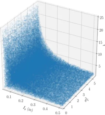
Fig. 1.Generated sample of size 𝑃=105 _of _{geostatistical} _parameters _m₌

(𝜎2

𝑌,𝐼y,𝜆)drawnfromajointpdf𝜋(m).Eachrealizationisusedtogetherwith

anassociatedR-realizationtocreatealog-hydraulicconductivityﬁeldonwhich ﬂowandtransportsimulationsareperformed.

2.4.1. Generationofhydraulicconductivityﬁelds

The log-hydraulic conductivity ﬁeld realizations 𝑌(x ) are gener-atedusing thefast circulantembeddingtechnique (seeDietrichand Newsam,1997fordetails).Agivenrealizationdependsonthe speci-ﬁedgeostatisticalmodelparametersandR ;a250×250arandomdraw fromastandardnormaldistribution.Thegeostatisticalmodel parame-tersdeterminethespatialregularity(smoothnessclass),while R deter-minesthelocationsofhighandlowlog-hydraulicconductivityvalues relativetothemeanvalue𝜇Yofthegeostatisticalmodel.Here𝜇Yis

ﬁxedat-6whileremainingparametersaretreatedasrandomvariables

m =(𝜎2

Y,𝐼y,𝜆)describedbyajoint probabilitydensityfunction(PDF) 𝜋(m ).Thevariance𝜎2

𝑌 israndomlydrawnfromauniformPDFwith

sup-port[0,5.5],theintegralscale𝐼yisdrawnfromalog-uniformPDFwith

support[L/25,L/2]m,andtheanisotropyfactor𝜆 (=𝐼_𝑥∕𝐼y)isdrawn

fromauniformPDFwithsupport[1,𝐿∕𝐼y](i.e.,conditionallyon𝐼y).

Thediscretizationimpliesthatheterogeneitiesobtainedwiththe small-estintegralscalesareresolvedwithatleast10cellsineachdirection. Thelog-uniformdistributionof𝐼y isherechosentofavorrealizations

withﬁnelystructuredﬁelds.Thegeneratedsampleofthegeostatistical modelparametersofsize𝑃=105_is_represented_in_Fig.₁_._Note_that_each

drawisassociatedwithauniqueR ,whichtogetherformalog-hydraulic conductivityﬁeldrealization.

2.4.2. Flowsimulations

The groundwater flow equation (Eq. (3)) is solved numeri-cally using the open-source finite-difference solver MODFLOW-2005 (Harbaugh,2005).Theprescribedboundaryconditionsareahorizontal headgradientof0.05inducingflowfromlefttorightandno-flow con-ditionsforthetopandbottomboundaries.Theheadgradientvaluewas chosensuchthatforahomogeneousfieldequaltoexp(𝜇Y)thetracer

ar-rivaltimeoccursapproximatelyathalfofthesimulatedtime-duration ofthetracerexperiment.Inthesimulations,thehydraulicconductivity betweentwoadjacentcellsistakenastheirharmonicmean.Thechosen

(5)

numericalschemeusedtosolvethesystemoflinearequationsis the preconditionedconjugategradientmethod(Hill,1990).

2.4.3. Transportsimulations

The advection-diﬀusion equation (Eq. (5)) is solved using the groundwater solute transport simulator package MT3D-USGS (Bedekar etal., 2016). Theinitial condition is a homogeneous con-centration ﬁeld of 0.01g l−1 _and _the _boundary _conditions _are: _(i)

constantconcentrationof1gl−1_along _the_left_boundary_(ii)_no-ﬂux

alongthetopandbottomboundariesand(iii)free-fluxalongtheright boundary.Theporosityisassumedconstantandequalto0.3.Forthe advectionterminEq.(5),thethird-orderTotalVariationDiminishing (TVD) approach(CoxandNishikawa,1991) isused.TheTVD solver wasfoundtobeveryrobustandshowedminimalnumericaldispersion when benchmarked against planar fronts. Nevertheless, in order to mask the small numerical dispersion, the diffusion coefficient was slightly increased from 𝐷𝑚=1.6× 10−9 m2 s−1 (the standard value

forthediffusioncoefficientofsaltinwater)to𝐷𝑚=2× 10−8m2 s−1. Thelatter(larger)valueisobtainedbyfitting theanalyticalsolution foraconcentrationprofileforastepinjectionin1-D(e.g.,Ogataand Banks,1961)toaTVD-calculatedconcentrationprofileobtainedfora homogeneoushydraulicconductivityfieldequalto𝜇Ywhenthe

diﬀu-sioncoeﬃcientisimposedtobetheoneofsaltinwater.Eachsimulated tracerexperimentlastsfor4×103_s_and_during_this_time_period,₄₀₀

equidistantsamples𝑐_𝑖(x )(𝑖=1,…,400)ofthesimulatedconcentration ﬁeldsarerecordedattimes𝑡=(𝑖−1)Δ𝑡,withΔ𝑡=4× 103_s∕400₌₁₀_s_.

The injected tracer typicallydoes not fully replace the initial back-groundtracerattheendofthesimulationperiod.Thisisaconsequence oftheshortsimulationtimeimposedbycomputationalconstraintsand large low-velocity regions.The meanPéclet numberis ~ 6 ×103_,

deﬁned as 𝑃𝑒= _𝐷̄𝑢

𝑚,where ̄𝑢 is the tracervelocity for the constant

hydraulicconductivityﬁeld.

2.4.4. Electricalsimulations

Foreachsampledconcentrationfield𝑐_𝑖(x ),the2-Dsquaredomain isalternativelyexcitedbyimposinganelectricalpotentialdifferenceof 1Vwithapairoflineelectrodesalongeithertheverticalor horizon-talboundariesofthesample.Theremainingboundariesareprescribed zeroelectricalpotentialgradientnormaltotheboundaries.The result-ingelectricalpotentialfields𝜙𝐻

𝑖 (x )and𝜙𝑉𝑖(x )associatedtothe

horizon-talandverticalmodes,respectively,arecomputedbynumerically solv-ingtheLaplaceequation(Eq.(8))withtheﬁnite-elementsolver mod-uleofthePythonlibrarypyGIMLi(Rückeretal.,2017).Forsimplicity, theinputelectricalconductivitydistribution𝜎𝑖(x ),usedforsolvingthe boundary-valueproblemsateachtimestepisassumedtobeperfectly andlinearlyrelatedtothetransportsimulationoutput𝑐𝑖(x ).The

result-ingnormalizeddimensionlesstime-seriesdenotedas𝜎H_,_𝜎V_and_M_vary

within[0.01,1].Thedatagenerationissummarizedbythepseudo-code inAlgorithm1.

3. Inference problem

Weareinterestedinassessingtowhatextentthetime-series𝜎H_,_𝜎V

andMmayconstrainthegeostatisticalparameters m =(𝜎2

Y,𝐼y,𝜆).We

considerthefollowingﬁvecombinationsoftime-series:

d _𝐻∶={𝜎𝐻},

d _𝑉 ∶={𝜎𝑉},

d _𝑀∶={𝑀},

d _𝐻𝑉 ∶={𝜎𝐻,𝜎𝑉},

d _𝐻𝑉_𝑀∶={𝜎𝐻,𝜎𝑉,𝑀}.

Thedatavectors d _𝐻,d _𝑉 and d _𝑀 areusedtoassesstheindividual performanceofeachtypeof time-series; d _𝐻𝑉 is usedtoevaluatethe

Algorithm 1: Datagenerationprocedure.

for 𝑗=1to105_do

Draw geostatistical model realization m =(𝜎2

𝑌,𝐼y,𝜆)

andR

Generate hydraulic conductivity field𝐾(x ) Simulate steady-state Eulerian flow fieldq (x )

for 𝑖=1to400 do

Specify sampling time 𝑡 as 𝑡=(𝑖−1)Δ𝑡 Simulate concentration field 𝑐_𝑖(x ) Compute𝑀_𝑖,𝜎𝐻_𝑖 and𝜎_𝑖𝑉

end

Save 𝐾(x )

Save concentration field time-series

C =[𝑐1(x ),…,𝑐400(x )]

Save time-series of mass breakthrough

𝑀=[𝑀1,…,𝑀400] and electrical conductivity

𝜎𝐻₌_[_𝜎𝐻

1 ,…,𝜎400𝐻] and𝜎𝑉 =[𝜎𝑉1,…,𝜎𝑉400]

end

performanceofelectricaldataaloneand d _𝐻𝑉_𝑀isusedtoevaluatethe valueofusingallthedataatthesametime.Wecasttheproblemasa Bayesianinferenceframeworkasoutlinedbelow.

3.1. Bayesianinferenceframework

In a ﬁnite-dimensional Bayesian inference framework, a model is described in termsof M random variables with realizations m = (𝑚1,…,𝑚𝑀)thatcan beused asinputtoa physicalforward

simula-torproducingNsimulateddata d 𝑠𝑖𝑚=(m )(e.g.,Gelmanetal.,2013; Tarantola, 2005).Theprior probability density function𝜋(m ) is up-dated using Bayes’ theorem to a posterior probability density func-tion𝜋(m |d𝑜𝑏𝑠₎_after_considering _the_observed _data_d𝑜𝑏𝑠₌₍_𝑑

1,…,𝑑𝑁)

usingalikelihoodfunction𝜋(d 𝑜𝑏𝑠|m).Thisfunctionevaluatesthe like-lihoodof any modelrealization given andthe residual error vector

e =d 𝑜𝑏𝑠−d 𝑠𝑖𝑚 andanassumedunderlyingobservational noisemodel (e.g.,Tarantola,2005).Bayes’theoreminitsunnormalizedformreads:

𝜋(m |d𝑜𝑏𝑠)∝𝜋(d 𝑜𝑏𝑠|m)𝜋(m ). (11)

In our context, the prior is given by the PDF described in Section2.4.1and d 𝑜𝑏𝑠isthenoise-contaminatedoutputoftheforward simulator,(m _𝑡),when evaluatedusing oneof thetestcases m _𝑡 de-scribedinSection4.2.Fortheelectricaltime-series,(m )isformedby thesequentialapplicationofthefollowingforwardmappings:(i)the re-alizationofthehydraulicconductivityfieldK(x ),(ii)solvingthe ground-waterflowEq.(3),(iii)theadvection-diffusionEq.(5),(iv)theLaplace Eq.(8)and(v)evaluatingtheequationsdefining𝜎H₍₉₎_and_𝜎V₍₁₀₎_. 3.2. Posteriordensityapproximation

InBayesianinference,MonteCarlo(MC)samplingcanbeusedto approximate𝜋(m |d𝑜𝑏𝑠₎_by_a_MC_integration_over_a_ﬁnite_sample_of_the

soughtdistribution(e.g.,MosegaardandTarantola,1995;Gelmanetal., 2013).ThesimplestapproachisAcceptance-RejectionSampling(ARS), whichconsistsofdrawingsamplesm proportionallytothepriordensity andacceptingthemassamplesoftheposteriordensityproportionally totheirlikelihood𝜋(d 𝑜𝑏𝑠|m).Thisisanexactsamplingmethod(e.g., Mosegaard andTarantola, 1995)andit canbe used oﬀ-lineusing a largeensembleofpriormodelrealizationsgiventhat,unlikeinaMarkov ChainMC(MCMC)samplingmethod,thereisnodependencebetween themodelproposals.Itsmaindisadvantageisthat,sincethe parame-tersearchis unguided(unlikeMCMC),theprobabilityof acceptance

(6)

decreasesexponentiallywiththedimensionalityMofthemodel param-eterspace.Asmoredimensionsareaddedtotheproblem,theratioof the(hyper)volumeof highlikelihoodvalues (regionsof large accep-tance probability),tothetotalvolumeof themodelspace,decreases exponentiallytozero(e.g.,Scales,1996;CurtisandLomax,2001).This so-calledcurseofdimensionalitymayresultinunrealistically-largeprior modelsamples,evenwhenaddressingonlyahandfulofparameters.In thecontextofthisstudy,weareinterestedinonlythreegeostatistical parameters(Section2.1)possiblysuggestingthatARScouldbeagood choice.

However,whenthescaleofthemodellingdomainisinsufficiently largecomparedtotheintegralscalesofthefieldY(x )under consider-ation, ergodicconditionsarenotfulfilledimplyingapotentiallyhigh dependenceonR (Section2.4.1).Thishigh-dimensionalvariableis dif-ferentforeachrealizationofY(x )anditultimatelycontrolsthe loca-tionsofhigh-andlowhydraulicconductivityregions.Evenifweare uninterestedin R assuch,itformspartofourdatagenerationprocess and,thus,itenterstheinferenceproblemasanuisancevariable(e.g., Gelmanetal.,2013)thatneedstobeaccountedfor.Consequently,our definitionoftheforwardsimulatorgivenabovehastobeexpandedto (m ,R ).Assumingindependenceof m and R examples,theactual in-ferenceproblemtosolvereads

𝜋(m ,R |d𝑜𝑏𝑠)∝𝜋(d 𝑜𝑏𝑠|m,R )𝜋(m )𝜋(R ). (12) Toobtainthesoughtdensity,weneedtomarginalize𝜋(m ,R |d)with respectto R :

𝜋(m |d)=

∫ 𝜋(m ,R |d)𝑑R . (13) Duetoitshigherdimensionality(morethan62,500variablesinour examples),theproblemexpressedbyEq.(12)ispracticallyimpossible tohandlewiththeformalBayesianARSalgorithm.Forthisreason,we resorttoanapproximateversionoftheARSthatisoutlinedinthe fol-lowingsubsection.

3.2.1. ABCacceptance-rejectionsamplingalgorithm

TheARSalgorithmimplemented withinanApproximateBayesian Computational (ABC) framework, labelled Approximate Acceptance-RejectionSampling(AARS)algorithmfromnowon,isanapproximate samplingmethodthatproducesasmoothapproximationof𝜋(m |d).The readerisreferredto(Sissonetal.,2018)foranoverviewonABC meth-ods.TheAARSalgorithmrequirestwoadditionalinputs:(i)adistance metric𝜌(d 𝑠𝑖𝑚,d 𝑜𝑏𝑠)forcomparingthecalculateddatawiththeobserved dataand(ii)akerneldensityfunction K _ℎ(𝜌)forweightingthedistance metricanddeﬁninganacceptanceprobability.Together,theyreplace thelikelihoodfunction.

Inourwork,thedistancemetric𝜌(d 𝑠𝑖𝑚,d 𝑜𝑏𝑠)istakenastheL1-norm:

𝜌(d 𝑠𝑖𝑚,d 𝑜𝑏𝑠)= 1 𝑁 𝑁 ∑ 1 |d𝑠𝑖𝑚−d 𝑜𝑏𝑠| (14)

andtheKerneldensityischosentobeauniformfunction:

K _ℎ(𝜌)= {

1 0≤𝜌∕ℎ≤1

0 1<𝜌∕ℎ, (15)

wheretheacceptancebandwidthh ischosensuchthatthe0.5th per-centileofthedistributionof𝜌 orderedfromthelowesttothehighest distance areaccepted.Inourcase,thismeansthat K _ℎ(𝜌)acceptsthe modelsproducingtheS=500lowestdistancesoutoftheK=105

sam-pledpriorsamples.

TheAARSalgorithm,describedinpseudo-codeinAlgorithm2, pro-ceedssimilarlytotheformalARSalgorithm.

ConsideringAlgorithm2,itcanbenoticedthattheAARSalgorithm drawssamplesfromthejointdistribution

𝜋𝐴𝐴𝑅𝑆₍_m_,_R_,_d_|d𝑜𝑏𝑠₎₌_K

ℎ(𝜌)𝜋(d 𝑜𝑏𝑠|d,m ,R )𝜋(m )𝜋(R ), (16)

Algorithm 2: Approximate Acceptance-Rejection Sampling (AARS)algorithm.

for 𝑘=1,…,𝑃 do

Draw m (𝑘) from 𝜋(m ) and R (𝑘) from 𝜋(R )

Generate a data instance d = d 𝑠𝑖𝑚 from the underlying unobserved likelihood𝜋(d 𝑜𝑏𝑠|d,m (𝑘),R (𝑘))

Accept m (𝑘) with an acceptance probability

𝐴𝑃=K _ℎ(𝜌)

end

which,whenintegratedoverallgenerateddatainstancesgivestheAARS approximationofthe(R -marginalized)posteriordensity:

𝜋𝐴𝐴𝑅𝑆₍_m_|d𝑜𝑏𝑠₎₌

∫ 𝜋𝐴𝐴𝑅𝑆(m ,R ,d |d𝑜𝑏𝑠)𝑑d ; (17) or,

𝜋𝐴𝐴𝑅𝑆₍_m_|d𝑜𝑏𝑠₎₌_𝜋(_m₎

∫ K ℎ(𝜌)𝜋(d 𝑜𝑏𝑠|d,m ,R )𝑑d . (18)

AspointedoutbySissonetal.(2018),fromEq.(18)theAARScanbe interpretedasaformalBayesianARSalgorithmusinganapproximated likelihoodfunctionthatisaKernelDensityEstimation(KDE)ofthetrue likelihood:

𝜋𝐴𝐴𝑅𝑆₍_d𝑜𝑏𝑠_|m_,_R₎₌

∫ K ℎ(𝜌)𝜋(d 𝑜𝑏𝑠|d,m ,R )𝑑d . (19)

Forbuildingtheempiricalposteriorprobabilitydensities, we per-formKDEoverthesamplesobtainedfrom𝜋𝐴𝐴𝑅𝑆₍_m_|d𝑜𝑏𝑠₎_._For

consis-tency,thepriorPDF(Section2.4.1)is computedbyperformingKDE overthegenerated sampleofsize𝑃 =105_. _The_KDE_approach_is

de-scribedinthefollowingsubsection.

3.2.2. Multivariatekerneldensityestimation(KDE)

GivenasampleX ={x 1,…,x S}ofsizeSofM-variaterandomvectors

belongingtoacommondistributiondescribedbythedensityg,theKDE estimator̂𝑔ofgisgivenby(e.g.,WandandJones,1994)

̂𝑔H(x )= 1 S S ∑ 𝑖=1 K _H(x −x _𝑖), (20)

withtheestimatorfunction K Hdeﬁnedas: 𝐊𝐇(𝐱)=|𝐇|−

𝟏

𝟐𝐾(𝐇−𝟏𝟐𝐱), (21)

wherethekernelfunctionKisasymmetricmultivariatedensity. Fur-thermore,|H| isthedeterminantof theM×Mbandwidth matrix H ,

whichissymmetricandpositivedeﬁniteingeneraland,iftheM vari-ablesareassumedindependent,itisdiagonalwithentries H _𝑖givenas √

H _𝑖=ℎ𝜎_𝑖, whereh isthebandwidthparameterand𝜎i thestandard

deviationoftheithcomponentoftherandomvariable.

TheestimatorofEq.(20)isanaverageofkerneldensitiesthatare centeredatthesamplepointsandwhosedecayiscontrolledby H .The particularchoiceofKdoesnotsubstantiallyinﬂuencetheperformance oftheKDEapproach,butthechoiceofthebandwidthh,deﬁning H

(i.e.,thetailsofK),isamostcrucialaspect,giventhatunder-or over-smoothedestimatorswillbeproducedifitistakentoosmallorlarge, respectively(e.g.,WandandJones,1994).Inthepresentwork, Kis chosenasthestandardmultivariatenormalfunction

K H(x )=(2𝜋)− 𝑁 2|H|− 1 2𝑒𝑥𝑝 { −1 2x T_H−1_x } . (22)

Forh,acommonchoicewhendealingwithunimodaldistributions, astheonesexpectedinthisstudy,isbasedonSilverman’sruleofthumb (e.g.,Silverman,1986): ℎ𝑠=_𝑀4₊₂ 1 𝑀+4 𝑑−_𝑀+41 . (23)

(7)

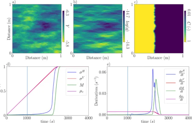
Fig.2.(Coloronline)(a)Weaklyheterogeneoushydraulicconductivityﬁeldwithgeostatisticalparameters(𝜎2

𝑌,𝐼y,𝜆)=(0.005,0.130m,3.179).(b)Corresponding

steady-stateflowfieldand(c)normalizedconcentrationfieldattime103_s._(d)_Time-series_of_the_horizontal_and_vertical_equivalent_electrical_{conductivity,}

mass-ﬂux,andmeantracerconcentration,denoted𝜎H_,_𝜎V_,_M_and_𝜇

c,respectively.Thelight-blueverticalline,alsopresentin(e),marksthetime103softheconcentration

ﬁeldshownin(c).(e)Time-derivativesof𝜎H_,_𝜎V_,_M_and_𝜇 c.

The reliabilityof theused information measure (Subsection 3.3) largelydependsonthequalityoftheinputdensityestimationsprovided bytheKDEapproach(e.g.,Budkaetal.,2011).Consideringthe trade-oﬀspertainingtothechoiceofh,amanualtuningprocesswas neces-sary,whichresultedinthechoiceofℎ=0.75ℎ_𝑠fortheresultspresented herein.

3.3. Informationmeasure:Kullback–Leiblerdivergence

Thedegreeofknowledgebroughtbytheobserveddatad 𝑜𝑏𝑠 pertain-ingtothegeostatisticalmodelparametersisevaluatedbycomparingour approximationof𝜋(m |d𝑜𝑏𝑠)with𝜋(m ).TheKullback–Leiblerdivergence (KLD)(KullbackandLeibler,1951),alsotermedRelativeInformation Content(Tarantola,2005),isprobablythemostwidelyused quantita-tivemeasureforcomparingPDFs:

𝐾𝐿𝐷(𝜋(m |d𝑜𝑏𝑠);𝜋(m ))= ∫ 𝜋(m |d𝑜𝑏𝑠)𝑙𝑛 ( 𝜋(m |d𝑜𝑏𝑠) 𝜋(m ) ) 𝑑m , (24)

wherethebaseofthelogarithmistakenase,givingtheinformation in unitsof nats (e.g.,Cover andThomas, 2012).The integration of Eq.(10) is performedoverthesupport ofthedensitiesandtheKLD isﬁniteasthesupportof𝜋(m |d𝑜𝑏𝑠)iscontainedinthesupportof𝜋(m ) (e.g.,CoverandThomas,2012).TheKLDiszerowhen𝜋(m |d𝑜𝑏𝑠₎_{≡ 𝜋(}_m₎

(i.e.,thedatacarrynoinformationaboutthemodelparameters)andit increasesastheposterior becomesmorecompactwithrespecttothe priorasaconsequenceofconditioningtothedata.Notethatwhenthe priorandposteriordensitiesareGaussianwiththesamemean,butthe standarddeviationoftheposteriorishalfthestandarddeviationofthe prior,thentheKLDis0.27nats.

Sinceoursamplesaredrawnfromapproximateposteriordensities

𝜋𝐴𝐴𝑅𝑆₍_m_|d𝑜𝑏𝑠₎_that_are_KDE_(i.e.,_smoothed)_versions_of_the_target

den-sities𝜋(m |d𝑜𝑏𝑠)(Eq.(18)),thechosenAARSapproachprovidesa con-servativeframeworkforassessingtheinformationcontentintermsof

theKLDmeasure,sinceitisalwaystruethat

𝐾𝐿𝐷(𝜋𝐴𝐴𝑅𝑆₍_m_|d𝑜𝑏𝑠_);_𝜋(_m₎₎_<_{𝐾𝐿𝐷(}_𝜋(_m_|d𝑜𝑏𝑠_);_𝜋(_m₎₎_, ₍₂₅₎

whichimpliesthattheinformationcontentintheconsideredtime-series isatleastaslargeastheestimatesobtainedbyouranalysis.

4. Results

Weﬁrstshowtwoexamplesofgenerateddataforend-membercases ofweakandstronghydraulicheterogeneity.Then,wedescribethe re-sultsobtainedfordiﬀerentgeostatisticalparametervaluecombinations intermsoftheKLDandbiasmeasures.Indoingso,wediscussresults obtainedforone R -realization,aswellasensemblestatisticsdeduced from50 R -realizations.

4.1. Twoexamplesofgenerateddata

Fig.2showsanexampleofdataobtainedforaweaklyheterogeneous hydraulic conductivity ﬁeld with (𝜎_𝑌2,𝐼y,𝜆)=(0.005,0.130m,3.179)

(Fig.2a),resultinginanapproximatelyconstantflowfield(Fig.2b).The correspondingconcentrationfield,shownatthesamplingtime103_s,

whenthetraceroccupiesapproximately50%ofthemodeldomain, dis-playsanoverallplanarfront(Fig.2c).

Thetime-seriesof𝜎H_and_𝜎V₍_Fig.₂_d)_evolve_according_to_the_lower

andupperWienerbounds.Theseupscalingformulasforlaminated ma-terials(e.g.,MiltonandSawicki,2003)correspondtotheharmonicand arithmeticmeansofthelocalelectricalconductivities,respectively.The arithmeticaveraginggoverning𝜎V_is_manifested_by_linear_scaling_with

time.Inthiscase,𝜎V_forms_an_almost_perfect_predictor_of_the_mean

salin-ity(𝜇c)withinthesample.𝜎H,onthecontrary,stronglyunderestimates 𝜇c.Forthiscase,themeanvelocityofthetracerfrontisgivenbythe

time-derivativeof𝜎V₍_Fig.₂_e),_information_that_is_available_before_the

(8)

Fig.3. (Coloronline)(a)Stronglyheterogeneoushydraulicconductivityﬁeld,deﬁnedwithgeostatisticalparameters(𝜎2

𝑌,𝐼y,𝜆)=(5.111,0.085m,1.028).(b)

Corre-spondingsteady-stateflowfieldand(c)normalizedconcentrationfieldattime103_s._(d)_Time-series_of_the_horizontal_and_vertical_equivalent_electrical_{conductivity,}

mass-ﬂux,andmeantracerconcentration,denoted𝜎H_,_𝜎V_,_M_and_𝜇

c,respectively.Thelight-blueverticalline,alsopresentin(e),marksthetime103s,ofthe

concentrationﬁeldin(c).(e)Time-derivativesof𝜎H_,_𝜎V_,_M_and_𝜇

c.Thelargepeaksexhibitedby𝑑𝜎

𝐻

𝑑𝑡 and𝑑𝑀𝑑𝑡 approximatelycoincidewiththeﬁrstarrivalofthe

tracerattheoutlet.

Theseeasilyinterpretableresultsarenowcontrastedwiththose ob-tainedforastronglyheterogeneoushydraulicconductivityfield,defined with (𝜎2_𝑌,𝐼y,𝜆)=(5.111,0.085m,1.028). The resulting fieldhas

small-scale structuresandis close toisotropic(Fig.3a). Yet itsassociated flowfieldexhibitspronouncedchanneling(Fig.3b)resultinginahighly heterogeneousconcentrationfield(Fig.3c).Neither𝜎H_nor_𝜎V_follow

anyknownupscalinglaw.TheybothstarttovarymuchearlierthanM

(Fig.2d),whichonlyreactswhenthetracerarrivesattheoutlet.These earlyvariationsareclearlyseeninthetime-derivativesofthe electri-calresponses(Fig.2e),whicharenon-zerofromthemomentthetracer injectionstartsandexhibitsmallpeaksthatarerelatedtointernal con-nectioneventsofthesolutethatareinvisibletoM.Both𝜎H_and_M_show

asteepincreasearound103_s,_and_a_large_peak_in_their_{time-derivatives,}

correspondingtoearlybreakthrougharrival.Forthiscase,𝜇cisatearly

timesmuchlargerthanalldataandisasymptoticallyapproximatedby

M,followedinorderofmagnitudeby𝜎H_and_𝜎V_. 4.2. Testcases

WenowapplytheBayesianinferenceapproachusingthreediﬀerent combinationsofthegeostatisticalmodelparametervalues:

(i) m 1∶=(4.70,0.06m,1.50).Thisleadstoastronglyheterogeneous

hydraulicconductivityﬁeldthatisapproximatelyisotropicand exhibitssmallstructures(Fig.4a).

(ii) 𝐦2∶=(0.80,0.06m,10.00). This leadstoa mildly-to-moderately

heterogeneous ﬁeld that exhibits a high degree of layering (Fig.4d).

(iii) 𝐦3∶=(4.70,0.38m,1.50). This leadsto a highlyheterogeneous

ﬁeldexhibitinglarge-scalestructures(Fig.4g).

InFig.4,examplerealizationsofgeneratedlog-hydraulic conductiv-ityfieldsforthethreetestcasesareshowntogetherwiththeir corre-spondingflowandconcentrationfields.

4.3. Informationassessmentofdatatypes

Foreachtestcaseofthemodelvectorm ,50datasetsd 𝑜𝑏𝑠_𝑗 (Section3) aresimulatedusing hydraulicconductivityfieldscreatedwith differ-entR -realizations.Theforwardresponsesarecontaminatedwithnoise havingzeromeanandameandeviationof0.005representing50%of thebaselineelectricalconductivity.Theevaluationofthedifferentdata typesandgeostatisticalparametervaluesisconsideredbothinterms oftheensembleofrealizations(ensembleperformance)andintermsof randomly-pickedsinglerealizations(i.e.,thefieldsshowninFig.4).In additiontotheestimatedjointposteriorPDF,wealsoconsiderthe cor-respondingmarginaldistributionstoevaluatetheabilityofthedatato constrainindividualgeostatisticalparameters.Forthemarginal analy-sis,wealsoconsiderarelativebiasmeasure,computedastheratioof themeanbiasofthemarginalposteriors,withrespecttothetruevalues of m ,tothemeanbiasofthemarginalpriorswithrespecttothetrue values.Fromnowon,wedropthesuperscript“obs” whenreferringto theobservedconditioningdata.

4.3.1. Testcasem1

Table1summarizestheresultsobtainedfortestcase m 1.

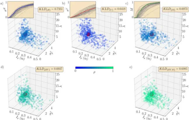
WhenconsideringthejointKLDsobtainedfortheensembleof real-izations,weﬁndthat d _𝐻𝑉 hasthelargestmeanKLD,closelyfollowed by d _𝐻𝑉_𝑀.Theleastinformativedatatype d _𝑀 hasameanKLDthatis ~ 75%oftheonefor d _𝐻𝑉,while d _𝐻and d _𝑉 havevaluesin-between. TheKLDstandarddeviations havesimilarvalues amongallthedata typesandrepresent ~ 20%ofthemeanvalues.

WenowturntotheresultsobtainedforthefieldsinFig.4a–candthe correspondingtime-serieshighlightedinFig.5a–c.Forthisspecific real-ization,theKLDsspanasmallrangeofonly ~ 13%.Also,theordering isdifferentandthemostandleastinformativedatasetsforthiscaseare

(9)

de-Fig.4. (a,d,f)Realizationsoflog-hydraulic conductivityfieldsand(b,e,h)associatedflow and(c,f,i)concentrationfieldsattime103_s

forthethreeevaluatedtestcases(a–c)m1,(d–

f)m2and(g–i)m3.Notethatthelocationsof

high-andlowhydraulicconductivityregions aregovernedbyrandomR-realizations.

Table1

KLDsandmeanrelativebiasesofm1forthediﬀerentconditioningdatatypes.Columns1and2show

themean𝜇KLDandstandarddeviation𝜎KLDoftheKLDsusingtheensembleofhydraulicconductivity

realizations.Column3showstheKLDvaluesforthejointposteriorPDFsusingonerealizationof theconditioningdataobtainedfromFig.4a–candhighlightedinFig.5a–c.Thesubsequentpairsof columnsshowthemarginalKLDvaluesandrelativemeanbiasesforthemarginalposteriorsofeach componentofm1usingthisspeciﬁcrealization.

Ensemble m 𝜎2

Y 𝐼 y ( m ) 𝜆

𝜇KLD 𝜎KLD KLD KLD Bias KLD Bias KLD Bias d_𝐻 0.8171 0.1445 0.7351 0.3754 0.5018 0.1418 0.7560 0.0904 0.8525 d_𝑉 0.8016 0.1131 0.6418 0.2617 0.6703 0.1021 0.6760 0.0675 1.2163 d_𝑀 0.6625 0.1580 0.6973 0.2153 0.8223 0.1771 0.5325 0.0980 1.1271 d_𝐻𝑉 0.8830 0.1352 0.6937 0.2501 0.6716 0.1536 0.7058 0.0899 0.7971 d𝐻𝑉𝑀 0.8712 0.1318 0.6985 0.2386 0.7232 0.1537 0.7189 0.1050 0.7672

viationsoftheKLDsdiscussedabove)thestochasticvariationsthatare inherentundernon-ergodicconditions.Thevariabilityinthegenerated datadue tovariationsin the R -realizations,foragivengeostatistical model,isindicatedbytheinsetsinFig.5a–c.

TheposteriormodelsamplesobtainedbytheAARSalgorithmand usedforbuildingtheempiricalposteriorPDFsforeachtypeofdataare showninFig.5.Thedensitydistributionofthese3-Dcloudsofpoints convey aqualitativeviewoftheabilityofthedifferentdatatypesto constrainthegeostatisticalparameters.Noeye-catchingdifferences dis-tinguishthedifferentpointclouds,reflectingtherathersimilarvalues oftheassociatedKLDs.

The KLDs computed for the marginal posterior PDFs, labelled marginalKLDsfromnowon,arethelargestfor𝜎2

Y,followedbyIyand𝜆,

thatonaverage,represent ~ 50%and~ 25%oftheKLDsof𝜎2

Y,

respec-tively.Weﬁndthat𝜎2

Yisbestconstrainedby d 𝐻,producingthelargest

marginalKLDandthesmallestbias.Forthisparameter,thepoorest per-formanceisachievedby d _𝑀 thathasboththesmallestmarginalKLD andthelargestbias.Thiscanbeseenintheestimatedmarginal poste-riorprobabilitydensity(Fig.6a)displayingamassdistributionwhichis thefurthestawayfromthetruevalue𝜎2

Y=4.70.ForIy,onthecontrary, d _𝑀 featuresthehighestmarginalKLDandthesmallestbias(Fig.6b). Theabilityofthedatatoconstrain𝜆 islow(Fig.6c)withd _𝐻𝑉_𝑀 featur-ingthehighestmarginalKLD.Therelativemeanbiasesarenegatively correlatedwiththeassociatedKLDmeasure,showingconsistency be-tweenthetwomeasures.

(10)

Fig.5.PosteriormodelparametervectorsamplesofsizeS=500obtainedbytheAARSalgorithmfortestcasem1=(4.7,0.06m,1.5)usingdiﬀerentdatasetsas

conditioningdata.Thecoloredcloudsofpointsrepresentthesamplesfordatasets(a)d_𝐻;(b)d_𝑉;(c)d_𝑀;(d)d_𝐻𝑉;(e)d_𝑉_𝑀;(f)d_𝐻𝑉_𝑀.Thecolormapencodesthe

L1distance𝜌 betweensimulatedandobserveddata,normalizedbytheminimumandmaximumvaluesof𝜌 ofthetestcase.Theinsetplotsof(a),(b)and(c)show,

respectively,the50realizationsoftime-series𝜎H_,_𝜎V_and_M_generated_for_m

1usingdiﬀerentR-realizations.Thedataconsideredhereforinferenceareshownby

thick-coloredcurves.TheresultingKLDvaluesaregivenforeachdataset.

Fig.6. (Coloronline)MarginalposteriorPDFsassociatedtoeachtypeofconditioningdatad_𝐻,d_𝑉,d_𝑀,d_𝐻𝑉,d_𝑉_𝑀andd_𝐻𝑉_𝑀fortestcasem1=(4.7,0.06m,1.5).

MarginalpriorandposteriorPDFscorrespondingto(a)𝜎2

Y(b)I𝑦and(c)𝜆.

4.3.2. Testcasem₂

Table2summarizestheresultsobtainedfortestcasem 2.

WhenconsideringthejointposteriorKLDsfortheensemble,weﬁnd that d _HVMisthemostinformativedatasetfollowedbyd _Hand d _HV.Far behind,featuringmeanKLDsthatare ~ 60%ofd HVM,are d Vandd M.

Oftheindividualdatasets,weﬁndthat d Hismuchmoreinformative

than d _Vand d _M.Thestandarddeviationshavesimilarmagnitudesand represent∼ 20−35%ofthemeanvalues.

Wenowconsidertheresultsobtainedusingthetime-series(Fig.7a– c)obtainedfromtheﬁeldsinFig.4d–f.TherankingforthejointKLDs aresimilartotheensemblemeanKLDs,exceptthat d _H performsthe

best.Thepointcloudsoftheposteriorsamples(Fig.7)clearlyshows that d H(Fig.7a)constrainthegeostatisticalmodelparametersmuch

betterthan d V(Fig.7b)and d M(Fig.7c).

ThemarginalKLDsareagainthelargestfor𝜎2

Y,followedbythose

of 𝐼y and𝜆.Weﬁndthat𝜎Y2 is themost constrainedby d Handthe

leastconstrained by d M asreﬂectedbytheir marginalKLDsandthe

compactnessoftheirposterior PDFs(Fig.8a).AllthemarginalPDFs for𝜎2

Yexhibitasmallbiastowardslargervariances,withthesmallest

andlargestbiasesexhibitedfor d HVMand d M,respectively.For𝐼y,the

marginalKLDassociatedwithd Hiswell-abovetheothers(Fig.8b).The

secondmostandthirdmostbestperformingdatasetforthisparameter ared HVand d HVM,while d Mperformsthepoorest.ThemarginalKLDs

(11)

Table2

KLDsandmeanrelativebiasesofm_⨙forthediﬀerentconditioningdatatypes.Columns1and2show themean𝜇KLDandstandarddeviation𝜎KLDoftheKLDsusingtheensembleofhydraulicconductivity

realizations.Column3showstheKLDvaluesforthejointposteriorPDFsusingonerealizationof theconditioningdataobtainedfromFig.4d–fandhighlightedinFig.7a–c.Thesubsequentpairsof columnsshowthemarginalKLDvaluesandrelativemeanbiasesforthemarginalposteriorsofeach componentofm2usingthisspeciﬁcrealization.

Ensemble m 𝜎2

Y 𝐼 y ( m ) 𝜆

𝜇KLD 𝜎KLD KLD KLD Bias KLD Bias KLD Bias dH 2.1341 0.5027 2.3829 1.3179 0.3687 0.8065 0.0573 0.5979 0.0971 dV 1.4448 0.4425 1.1625 0.7427 0.4359 0.1115 0.6425 0.1003 0.7639 dM 1.3897 0.4768 1.0892 0.4866 0.4889 0.0875 0.6883 0.0952 0.8219 dHV 2.1114 0.4465 2.0030 0.9984 0.3019 0.6399 0.1306 0.5412 0.1657 dHVM 2.2256 0.4648 2.0741 1.0955 0.2452 0.6158 0.1417 0.4410 0.2640

Fig.7. PosteriormodelparametervectorsamplesofsizeS=500obtainedbytheAARSalgorithmfortestcase𝐦2=(0.80,0.06m,10.00)usingdiﬀerentdatasetsas

conditioningdata.Thecoloredcloudsofpointsrepresentthesamplesfordatasets(a)dH;(b)dV;(c)dM;(d)dHV;(e)dVM;(f)dHVM.ThecolormapencodestheL1

distance𝜌 betweensimulatedandobserveddata,normalizedbytheminimumandmaximumvaluesof𝜌 ofthetestcase.Theinsetplotsof(a),(b)and(c)show, respectively,the50realizationsoftime-series𝜎H_,_𝜎V_and_M_generated_for_m

thick-coloredcurves.TheresultingKLDvaluesaregivenforeachdataset.

andbiasesfor𝜆 (Fig.8b)followtherankingof𝐼y.Forthistestcase m 2,

thedatabetterconstrainthegeostatisticalparametersthanfortestcase

m 1asreﬂectedbygenerallymuchlargerKLDvalues.

4.3.3. Testcasem3

Table3summarizestheperformanceofthediﬀerentdatasetsfortest casem 3.

ConsideringtheensemblestatisticsofthejointposteriorKLDs,we ﬁndthat d _HVhasthelargestmeanKLD,closelyfollowedby d _HVMand

d H. Again, d M featuresthe smallestmeanKLDwith avalues thatis

~ 63% of that for d HV. The standarddeviations arevarying within

~ 15%andrepresent ~ 25%ofthemeanvalues.

Wenowconsidertheresultsfromthedatatime-series(Fig.9a–c) obtainedfromtheﬁeldsinFigs.4g–i.ThejointKLDford Histhelargest

closelyfollowedbyd HVand d HVM.TheirKLDsare ~ 30%higherthan

theothers.Thepointcloudsofposteriormodelrealizations(Fig.9)are

rathersimilar,buttheresultsobtainedfromd H(Fig.9a)aremore

com-pactcomparedto d Vand d M.Forinstancethereisminimalscatterin

the𝜆-direction(c.f.,Fig.9b)andthehigh𝜎2

Yisbetterconstrained(c.f.

Fig.9c).

ThemarginalKLDsareagainthehighestfor𝜎2

YfollowedbyIyand 𝜆.Therelativemeanbiasesshowasimilartrend,beingsmallestfor𝜎2

Y.

Themarginalprobabilitydensitiesfor𝜎2

Y(Fig.10a)showthat d Hbest

constrainthisparameter,followedbyd HVand d HVM.ThemarginalKLD

for d Hareonly ~ 10%largerthanfor d HV and d HVM,butitsbiasis

30%lower.Notealsothatd _Misstronglybiasedtowardstoolow𝜎2

Y.For Iyand𝜆,bothKLDsandbiasesindicatethat d H,d HVand d HVMarethe

(12)

Fig.8. (Coloronline)MarginalposteriorPDFsassociatedtoeachtypeofconditioningdatadH,dV,dM,dHV,dVManddHVMfortestcase𝐦2=(0.80,0.06m,10.00).

Table3

KLDsandmeanrelativebiasesof𝐦⨚forthediﬀerentconditioningdatatypes.Columns1and2show

themean𝜇KLDandstandarddeviation𝜎KLDoftheKLDsusingtheensembleofhydraulicconductivity

realizations.Column3showstheKLDvaluesforthejointposteriorPDFsusingonerealizationof theconditioningdataobtainedfromFigs.4g–iandhighlightedinFig.9a–c.Thesubsequentpairsof columnsshowthemarginalKLDvaluesandrelativemeanbiasesforthemarginalposteriorsofeach componentofm3usingthisspeciﬁcrealization.

Ensemble m 𝜎2

Y 𝐼 y ( m ) 𝜆

𝜇KLD 𝜎KLD KLD KLD Bias KLD Bias KLD Bias dH 1.1845 0.3195 1.0166 0.4818 0.3098 0.2681 0.6388 0.2031 0.3962 dV 1.0565 0.3313 0.7459 0.3046 0.6171 0.0488 0.9635 0.0356 1.0166 dM 0.8413 0.2798 0.6205 0.2019 0.7347 0.1949 0.6983 0.1296 0.5169 dHV 1.3462 0.3491 1.0123 0.4491 0.4202 0.2680 0.6577 0.2054 0.4002 dHVM 1.2932 0.3100 1.0068 0.4200 0.4429 0.2915 0.6164 0.2245 0.3647

Fig.9. PosteriormodelparametervectorsamplesofsizeS=500obtainedbytheAARSalgorithmfortestcase𝐦3=(4.70,0.38m,1.50)usingdiﬀerentdatasetsas

conditioningdata.Thecoloredcloudsofpointsrepresentthesamplesfordatasets(a)dH;(b)dV;(c)dM;(d)dHV;(e)dVM;(f)dHVM.ThecolormapencodestheL1

distance𝜌 betweensimulatedandobserveddata,normalizedbytheminimumandmaximumvaluesof𝜌 ofthetestcase.Theinsetplotsof(a),(b)and(c)show, respectively,the50realizationsoftime-series𝜎H_,_𝜎V_and_M_generated_for_m

(13)

Fig.10. (Coloronline)MarginalposteriorPDFsassociatedtoeachtypeofconditioningdatadH,dV,dM,dHV,dVManddHVMfortestcase𝐦3=(4.7,0.38m,1.5).

5. Discussion 5.1. Generalﬁndings

TheabsolutevaluesofthecomputedKLDsandbiasesaredependent onthechoicesmadewhenapproximatingtheposteriorprobability den-sities(Section2.2),suchasthewidthoftheacceptancekernelofthe AARSalgorithm(Algorithm2)andthebandwidthof thekernel den-sityfunctionusedtorepresenttheprobabilitydensities.Forthisreason, wefocusourdiscussionbelowonrelativediﬀerencesbetweendatasets andtestcases.Weﬁrstsummarizethemainresultsthatapplytoalltest casesbeforediscussingthetestcasesone-by-one.Afterthis,wediscuss broaderimplicationsofthisresearch.

Consideringtheensemblestatisticsof50hydraulicconductivity re-alizationsforeachtestcase,weﬁndthattheinformationcontentofd H

measuredbytheKLDishigherthan d V,whichinturnishigherthan d _Mforthethreetestcasesconsidered:m ₁(Table1), m ₂(Table2)and

m 3(Table3).Theaddedvalueofcombiningdiﬀerentdatatypes(d HV

and d HVM)isgenerallyfoundtobecomparativelylow.When

consider-ingindividualhydraulicconductivityrealizationsandassociatedfields (Fig.4),wegenerallyobtainrelativerankingsofthedifferentdatatypes thatareconsistentwiththoseof theensemble means.Giventhatwe considernon-ergodicmodeldomains,theactuallocationsofhigh-and lowhydraulicconductivitiesgovernedbythenuisancevariableR plays animportantroleinthedata-generatingprocess.Itsimpactis mani-festedbythecomparativelyhighstandarddeviationsoftheKLD esti-mates(Tables1–3)and(inthevariabilityofthegeneratedtime-series (Figs.5a–c,7a–cand9a–c).Despitethisinherentstochasticvariability, weconsistentlyfindthatthebestconstrainedparameteris𝜎2

Y,followed

byI_yand𝜆.Theindividualtestcasesarediscussedindetailbelow.

5.2. Lessonslearnedfromthethreetestcases

Testcase m ₁featuresahighlyheterogeneousfield𝐾(x )with rela-tivelysmallstructures(Fig.4a),forwhichonecouldpossiblyassume thatergodicconditionsarefullfilledandconsequentlythatthe geosta-tisticalparametersarewell-representedwithinthemodellingdomain, yet itcorresponds tothe least-constrained testcase. Indeed, the R -realization playshere averyimportantrole,implyingarather weak mappingfromthetime-seriestothegeostatisticalparametersof inter-est.Tounderstandthis,notefirstthat{𝜎H_}_and_{_𝜎V_}_are_only_sensitive

totheunderlyinggeostatisticalparametersthroughthesolutespreading patternsthattheseparametersinduce.Indeed,theelectricalresponses resultfromoptimalcurrentpatternsestablishedthroughoutthehighly

non-ergodicandtime-evolvingdistributionoflocalconcentrations(i.e., conductivities) thatare,in turn,drivenbytheflow field𝐪(x ). Asin theexampleinFig.2,thehydraulicconductivityfield𝐾(x )has small-scalestructuresandisclosetoisotropic(Fig.4a)butitsassociatedflow field𝐪(x )exhibitspronouncedchanneling(Fig.4b). Thistendencyof theflowfieldtoconcentrateinpreferentialflowchannelsforhigh𝜎2

𝑌

iswell-known(e.g.Cvetkovicetal.,1996).Hence,anergodic𝐾(x )is noguaranteeofwell-sensedgeostatisticalparameterswhenusing geo-electricallymonitoredsalinetracertests.Nevertheless,comparedtothe prior,theestimatedmarginalposteriordensitiessuggestthatthe geo-statisticalmodelthatneedsacomparativelyhigh𝜎2

Y(Fig.6a)andvery

smallorhighIy(Fig.6b)areunlikely.

Testcase m ₂correspondstoalayereddistributionofhydraulic con-ductivitywithamoderate𝜎2

Y.TheKLDs(Table2),andconsequently

theconstrainingnatureofthetime-series,aremuchhigherthanfortest cases m 1 (Table1)and m 3(Table3).For m 2,thesmallestvariations

between the R -realizationsareobserved (Fig.7a–c)sincethe actual locationoftheflowchannelsisofsecondaryimportanceinthe data-generatingprocess.Thehydraulicconductivityfield(Fig.4d)andits as-sociatedflowfield(Fig.4e)arevisuallymoresimilartoeachotherthan for m 1.Thisisaconsequenceofthelargeanisotropyfactorimposing

horizontallycontinuousstructureswithinwhichtheﬂow-ﬁeldchannels arenaturallydeveloped.Both{𝜎H_}_and_{_M_}_are_highly_sensitive_to_the

arrivalofhorizontalconnectionsthatareestablishedbythesolutewhen itarrivestotheoutlet.ConsideringthemarginalKLDs,weﬁndthathigh andlow𝜎2

Y-valuesareincompatiblewiththedata(Fig.8a),asislarge Iy.Forthistestcase m 2,𝜆 isparticularlyinterestingasitstruevalueis

highand,therefore,oflowpriorprobability(Fig.8c).Weseeastrong abilityofalltime-seriesincluding{𝜎H_}_to_constrain_this_parameter.

Testcase m ₃isahighlyheterogeneoustestcasethatdistinguishes itselffrom m 1 byitslarger Iy.Aconsequenceof theresulting larger

structuresisthatthegenerateddatavarywidelybetweenthediﬀerent hydraulicconductivityrealizations(seeinsetsinFig.9a–c).YettheKLDs (Table 3) arehigherthanfortestcase m 1.Consideringthemarginal

posteriorPDFs,alldatasetsindicate thattheunderlyinggeostatistical modelhasahigh𝜎2

Y(Fig.10a),atleastamoderatelyhighIy(Fig.10b)

and(thattheﬁeldisclosetoisotropic(Fig.10c).

5.3. Physicalinsightsandopenquestions

Inouridealizednumericalinvestigation,wefoundconsistentlythat geoelectricaldataperformedbetterthanmassbreakthroughdatain con-strainingthegeostatisticalparameters.Thisisaconsequenceofthefact that,foragivengeostatisticalmodel,theactualpositioningofhigh-and

(14)

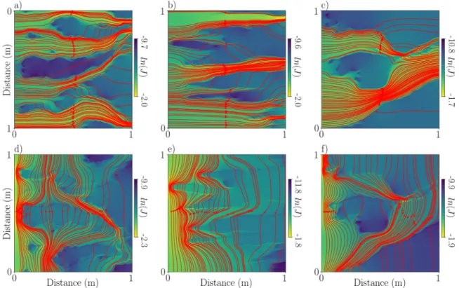
Fig.11. Naturallogarithmoftheabsolutevalueofthecurrentdensityﬁelds(andtheirstreamlines)resultingfromexcitingthesamplebothinthe(a–c)horizontal and(d–f)verticalmodes.TheelectricalconductivitydistributionisgivenbythesalineconcentrationﬁeldsshowninFig.4,thatis,attime103_s_for_the_three

evaluatedtestcases(a,d)m1(column1),(b,e)m2and(c,f)m3.

lowhydraulicconductivityfields,governedbythenuisancevariable R , hasalargerimpactonthemassbreakthroughdatathanonthe geoelec-tricaldata(e.g.,comparetheinsetsinFig.9a–c).Weunderstandthis asaconsequenceofthelocalflux-averagednatureofthetracer break-through,comparedtothemoreintegrativenon-linearvolume-averaging of theelectrical responsesover theconcentrationfield.Additionally, since{M}isonlysensitivetothetime-evolutionofthesolute concen-trationfieldattheoutlet,itcannotdeterminethecausalityofthearrival times,thatis,iftheyoriginatefromlargehorizontalcorrelationscales orfromhighvariance,forinstance.

Wealsofoundthat{𝜎H_}_always _has_a _higher_constraining_power

than{𝜎V_}._This_can_be_understood_by_noting_that_{_𝜎H_}_is_sensitive_to

electricalconductionpathscreatedbytheconcentrationﬁeldintheﬂow direction,leadingtoaverystrongsensitivitytotracerarrivalsatthe outlet(e.g.,Fig.2e,orthegenerallysteepslopesinthegenerated time-seriesin theinsetsof Figs. 5a, 7aand9a). InFig.11we plotthe generatedcurrentdensitydistributionsdetermining{𝜎H_}_and_{_𝜎V_}_for

theconcentrationﬁeldsshowninFigs.4c,fandj.Weseethatfor{𝜎H_}

(Figs.11a–c)thesupportofthecurrentdensityfield(i.e.theregions of highcurrent flow)is almostcoincidentwiththeareaoccupiedby theinvading tracerdrivenbytheflow-field. Thisdoesnot occurfor {𝜎V_}₍_Figs.₁₁_d-f),_indicating_why_{_𝜎H_}_is_more_informative_than_{_𝜎V_}.

Clearly,{𝜎V_}_results_from_current_patterns_that_are_mainly_constrained

byverticalconnectionbottlenecksthatbecomemorecommonfurther awayfromtheinletregion.Thiscanbeappreciatedbythehighdensity ofcurrentﬁeldstreamlinesobservedattheinletregionsinFigs.11d, 1111eand11f.Thissuggeststhatthemainabilityof{𝜎V_}_to_sense_the

geostatisticalparametersisthroughitssensitivitytothetrailingendof thetracerfront.Again,itistheconnectivity-aspectoftheelectricaldata thatisatplay.

Ourresultsalsosuggestastrongdependenceontheinjectiontype. Forapulseinjection,weexpect{𝜎H_}_to_be_much_less_informative,

com-paredtothepresentcontinuousinjectioncase,astherewillbeno hor-izontalconnectionsofsalinitytosense.Thatis,theconnectivity

cre-atedbyestablishingacontinuousconcentrationﬁeldacrossthedomain isveryhelpfulforelectrical-basedinferenceofgeostatisticalproperties fromtracertests.

Foralltestcases,weﬁndthat𝜎2

Yisthebestconstrainedparameter.

Thisisexplainedbythefactthat𝜎2

Ycontrolsthespreadingrateofthe

solute(e.g.,GelharandAxness,1983)andis,thus,aﬁrst-orderfeatureof thetime-series.Itwilldeterminethetime-spacingorpaceofoccurrence ofthehorizontalconnectioneventsassensedparticularlywellby{𝜎H_}.

However,alsothetrailingpartofthetracerﬁeldassensedby{𝜎V_}_is

aﬀectedby𝜎2

Y.

Oneopenquestionistowhatextenttheelectricaldatacanconstrain mixingandspreading.Intuitively,thereshouldbeastrongsensitivity tothespreadingwidthas𝜎H_is_highly_sensitive_to_the_front_of_the_tracer

plumeand𝜎V_to_its_end._Since_solute_spreading_ultimately_controls

so-lutemixing(e.g.,Villermaux,2019),thehighsensitivityoftheelectrical datatotheformerindicatesthatthesedataareabletoatleastquantify themixingpotentialofthesolute(e.g.,deDreuzyetal.,2012).This willbethetopicoffutureresearch.Furthermore,theequivalent electri-calconductivitytensortime-seriesisdeterminedbythetime-evolution oftheconcentrationfield,whichinturnisdrivenbytheflow-field.This suggeststhatthattheelectricaldatamightbemorestronglyrelatedwith theflow-fieldthanthegeostatisticalmodeloflog-hydraulic conductiv-ity.Inthefuture,weplantostudythegeoelectricalsensitivityto flow-fielddescriptors(e.g.,Koponenetal.,1996;Englertetal.,2006). Sim-ilarly,wewouldliketorelatetheelectricaldatatoconcentrationfield descriptors.However,astheconcentrationfieldistime-variant,thisis morechallengingtosummarizethanthesteady-stateflowfield.One possibilityistorelateittothespatialdistributionoflocalizedtemporal momentsofthesoluteconcentrationfield(CirpkaandKitanidis,2000).

5.4. Implicationsforﬁeld-basedstudies

Ourworkhasseveralimplicationsforﬁeld-basedand laboratory-basedelectricaltime-lapsemonitoringof tracertests.Theﬁrstisthat