Quasi‐dynamic versus fully dynamic simulations of earthquakes and aseismic slip with and without enhanced coseismic weakening

HAL Id: hal-03079566

https://hal.archives-ouvertes.fr/hal-03079566

Submitted on 17 Jan 2021

HAL is a multi-disciplinary open access

archive for the deposit and dissemination of

sci-entific research documents, whether they are

pub-lished or not. The documents may come from

teaching and research institutions in France or

abroad, or from public or private research centers.

L’archive ouverte pluridisciplinaire HAL, est

destinée au dépôt et à la diffusion de documents

scientifiques de niveau recherche, publiés ou non,

émanant des établissements d’enseignement et de

recherche français ou étrangers, des laboratoires

publics ou privés.

enhanced coseismic weakening

Marion Y. Thomas, Nadia Lapusta, Hiroyuki Noda, Jean-philippe Avouac

To cite this version:

Marion Y. Thomas, Nadia Lapusta, Hiroyuki Noda, Jean-philippe Avouac. Quasi-dynamic versus

fully dynamic simulations of earthquakes and aseismic slip with and without enhanced coseismic

weakening. Journal of Geophysical Research : Solid Earth, American Geophysical Union, 2014, 119

(3), pp.1986-2004. �10.1002/2013JB010615�. �hal-03079566�

RESEARCH ARTICLE

10.1002/2013JB010615

Key Points:

•With enhanced weakening, fully dynamic runs produce pulse-like ruptures

•In the same cases, quasi-dynamic runs yield much larger crack-like ruptures

•The rupture-mode differences dramatically affect long-term fault behavior

Correspondence to: M. Thomas,

marion.caltech@gmail.com

Citation:

Thomas, M. Y., N. Lapusta, H. Noda, and J.-P. Avouac (2014), Quasi-dynamic versus fully dynamic simulations of earthquakes and aseismic slip with and without enhanced coseismic weaken-ing, J. Geophys. Res. Solid Earth, 119, 1986–2004, doi:10.1002/2013JB010615.

Received 28 AUG 2013 Accepted 22 JAN 2014

Accepted article online 28 JAN 2014 Published online 20 MAR 2014

Quasi-dynamic versus fully dynamic simulations

of earthquakes and aseismic slip with and

without enhanced coseismic weakening

Marion Y. Thomas1_{, Nadia Lapusta}1,2_{, Hiroyuki Noda}3_{, and Jean-Philippe Avouac}1

1_{Division of Geological and Planetary Science, California Institute of Technology, Pasadena, California, USA,}2_{Division of} Engineering and Applied Science, California Institute of Technology, Pasadena, California, USA,3Institute for Research on Earth Evolution, Japan Agency for Marine-Earth Science and Technology, Yokohama, Japan

Abstract

Physics-based numerical simulations of earthquakes and slow slip, coupled with field observations and laboratory experiments, can, in principle, be used to determine fault properties and potential fault behaviors. Because of the computational cost of simulating inertial wave-mediated effects, their representation is often simplified. The quasi-dynamic (QD) approach approximately accounts for inertial effects through a radiation damping term. We compare QD and fully dynamic (FD) simulations by exploring the long-term behavior of rate-and-state fault models with and without additional weakening during seismic slip. The models incorporate a velocity-strengthening (VS) patch in a velocity-weakening (VW) zone, to consider rupture interaction with a slip-inhibiting heterogeneity. Without additional weakening, the QD and FD approaches generate qualitatively similar slip patterns with quantitative differences, such as slower slip velocities and rupture speeds during earthquakes and more propensity for rupture arrest at the VS patch in the QD cases. Simulations with additional coseismic weakening produce qualitatively different patterns of earthquakes, with near-periodic pulse-like events in the FD simulations and much larger crack-like events accompanied by smaller events in the QD simulations. This is because the FD simulations with additional weakening allow earthquake rupture to propagate at a much lower level of prestress than the QD simulations. The resulting much larger ruptures in the QD simulations are more likely to propagate through the VS patch, unlike for the cases with no additional weakening. Overall, the QD approach should be used with caution, as the QD simulation results could drastically differ from the true response of the physical model considered.

1. Introduction

The expanding set of seismic and geodetic observations provides increasingly better insight into the vari-ability of fault slip behaviors over a wide range of temporal and spatial scales. These observations allow us to image the rapid coseismic phase, which involves slip rates of the order of 1 m/s and generates seismic waves, as well as the interseismic and postseismic phases which involve slip rates of the order of mm/yr to m/yr and duration of years to centuries [e.g., Chlieh et al., 2008; Perfettini et al., 2010; Loveless and Meade, 2011]. These observations suggest a complex pattern of slip, with a fault interface likely consisting of interfingered patches that either creep at a low rate, without seismic radiation, or remain locked during the interseis-mic period and rupture seisinterseis-mically. It has been observed that this segmentation has a strong influence on seismic rupture patterns [Burgmann et al., 2005; Hetland and Hager, 2006; Chlieh et al., 2008; Kaneko et

al., 2010; Perfettini et al., 2010; Chlieh et al., 2011; Loveless and Meade, 2011]: locked segments may rupture

independently or together with neighboring patches, producing irregular earthquakes of different sizes. This complex behavior arises from the interaction of stress transfer, levels of prestress, and fault friction properties [Rundle et al., 1984; Cochard and Madariaga, 1996; Ariyoshi et al., 2009; Kaneko et al., 2010]. Understanding the partitioning between seismic and aseismic slip is an important issue in seismotectonics, since it is a key factor in determining the seismic potential of any fault. Theoretical and numerical techniques now exist to simulate fault slip and reproduce this partitioning. Numerical models can be vali-dated and calibrated through comparison with geodetic, seismological, and geological observations [Barbot

In such modeling, it is essential to incorporate all stages of the fault slip, including seismic as well as preseis-mic, postseispreseis-mic, and interseismic slow slip, into a single physics-based model, as they interact and influence each other. Indeed, prestress inherited from aseismic slip history and prior seismic events likely determines where earthquakes will nucleate and how far their rupture will propagate. However, numerical simulations that account for full inertial (wave) effects during seismic events as well as long-term slow slip are challeng-ing because of the wide range of temporal and spatial scales involved [Lapusta et al., 2000]. That is why the representation of dynamic effects or the aseismic fault slip between earthquakes is often simplified [e.g.,

Shibazaki and Matsuura, 1992; Cochard and Madariaga, 1996; Kato, 2004; Duan and Oglesby, 2005; Liu and Rice, 2005; Hillers et al., 2006; Ziv and Cochard, 2006]. In quasi-static simulations, a series of static problems

is solved, with the loading advanced in time. Such methods cannot simulate fast slip during seismic events, and earthquakes have to be prescribed in a kinematic fashion. The physical insight offered by such meth-ods is therefore limited. A common more robust approximation is the quasi-dynamic (QD) model [Rice, 1993; Ben-Zion and Rice, 1995; Rice and Ben-Zion, 1996; Hori et al., 2004; Kato, 2004; Hillers et al., 2006; Ziv

and Cochard, 2006] in which the wave-mediated stress transfers are ignored. In the QD simulations,

iner-tial effects during simulated earthquakes are approximately accounted for through a radiation damping term. This method allows computing the long-term histories of fault slip, including the seismic phase, with-out having to pay significant additional memory and computational costs associated with modeling true wave-mediated effects. The QD methods thus allow for self-consistent modeling of all phases of fault slip at a reasonable computational cost.

However, the question arises as to how the results of simulations are influenced by ignoring the wave-mediated transient part of the dynamic response. Wave-mediated stress transfers play a key role in concentrating stress at the tip of the propagating rupture [Lapusta et al., 2000; Lapusta and Liu, 2009] or creating appropriate stress conditions for rupture transition to supershear speeds [e.g., Andrews, 1976;

Harris and Day, 1997; Xia et al., 2004; Dunham, 2007; Liu and Lapusta, 2008]. Hence, the wave-mediated stress

transfers can qualitatively define the model response.

Here we explore our hypothesis that the fully dynamic (FD) simulations are needed to capture even the basic qualitative features of the response in such cases and that the usefulness of the QD simulations for capturing even the qualitative features of the response is limited. To that end, we study two different physical models. In the first model, only the standard rate-and-state friction laws [Dieterich, 1979; Ruina, 1983; Dieterich, 2007, and references therein] are used, as in Lapusta et al. [2000] and Lapusta and Liu [2009]. In the second model, we include enhanced dynamic weakening motivated by flash heating [Rice, 2006], which has been shown to result in self-healing pulses on low-prestressed faults [Zheng and Rice, 1998; Noda et al., 2009; Rojas et

al., 2009]. The self-healing mode is generated through appropriate stress transfers by dynamic waves, and

hence the QD approach should not be able to capture it appropriately. We indeed find that the QD and fully dynamic (FD) simulations produce dramatically different results in the model with the enhanced weaken-ing. Similarly, dramatic differences between the QD and FD approaches are expected in other situations where wave-mediated effects play a significant role, such as in the models with transitions to supershear speeds. We also consider how the QD and FD simulations compare with respect to rupture interaction with a potential local barrier in the form of a fault region with velocity-strengthening friction, following the study of Kaneko et al. [2010].

Our methodology is described in section 2, with a particular emphasis on the differences between the FD and QD approaches. Section 3 presents the FD and QD simulations of earthquake sequences with the stan-dard rate-and-state laws. In section 4, we consider how fault response compares when enhanced coseismic weakening is added in the FD and QD cases. The reasons for the dramatic differences between FD and QD simulations with enhanced weakening are discussed in section 5. In section 6 we explore the ability of the earthquake rupture to propagate over faults with heterogeneous properties for the two different friction laws models used in this paper, with or without full wave-mediated effects. Our findings are summarized in section 7.

2. Methodology

Our simulations are conducted following the methodological developments by Lapusta et al. [2000], Lapusta

but coseismically weak fault: lw-stress/low-heat operation, typical stress drops, and importance of earth-quake nulceation, submitted to Journal of Geophysical Research, 2014, herein after referred to as Lapusta et al., submitted manuscript, 2014).

2.1. Fully Dynamic Versus Quasi-dynamic Formulation

We consider a 2-D antiplane (Mode III) model, with a 1-D fault embedded in a 2-D uniform, isotropic, elastic medium. Earthquakes occur spontaneously on the fault subject to slow tectonic loading. The model has been fully described by Lapusta et al. [2000]. Nevertheless, in order to understand the difference between QD and FD formulations, it is useful to recall the underlying elastodynamic equations. We assume purely dip-slip motion on a fault, which coincides with the x-z plane of a Cartesian coordinate system xyz. The only nonzero displacement u_x(y, z, t) is along strike (parallel to the x direction). Then the time-dependent relative

slip𝛿(z, t) corresponds to the displacement discontinuity 𝛿(z, t) = u_x(0+_{, z, t)−u}

x(0−, z, t). The relevant shear

stress on the fault plane𝜏(z, t) = 𝜎_xy(0, z, t) is expressed as the sum of a loading term 𝜏0_{(z, t), i.e., the stress}

that would act in absence of any displacement discontinuity on the fault plane y = 0, and some additional terms related to slip𝛿(z, t) [Perrin et al., 1995; Cochard and Madariaga, 1996; Lapusta et al., 2000]:

𝜏(z, t) = 𝜏0_{(z, t) + f(z, t) −} 𝜇

2c_sV(z, t), (1)

where𝜇 is the shear modulus, csis the shear wave speed, and V(z, t) = 𝜕𝛿(z, t)∕𝜕t is the slip rate. In

equation (1), the functional f (z, t) incorporates most of the elastodynamic response and represents the stress transfer along the fault through waves. It is a linear functional of prior slip𝛿′_(z′_{, t}′_{) over the causality}

cone that expresses the stress transfer due to a rupture. The third term,_2c𝜇V(z, t), represents the radiation damping term (energy radiated by waves in the medium) [Rice, 1993]. Explicit extraction of that term from the functional f (z, t) avoids singularities of the convolution integrals [Cochard and Madariaga, 1996]. The difference between the FD and QD models lies in the expression of the stress-transfer functional f (z, t), which involves a double convolution integral in space and time. In the spectral domain, f (z, t) is related to

𝛿(z, t) by a single convolution integral in time when slip and the functional are represented as a truncated

Fourier series in space [Perrin et al., 1995]. This is very advantageous, as convolution integrals are the most computationally demanding part of the elastodynamic analysis. Let us write the following:

𝛿(z, t) = N∕2 ∑ n=−N∕2 D_n(t)eiknz, ₍₂₎ f (z, t) = N∕2 ∑ n=−N∕2 Fn(t)eiknz, kn= 2𝜋n 𝜆 , (3)

where𝜆 is the length of the fault domain, replicated periodically and discretized into N (even) elements. The period𝜆 has to be larger than the domain over which the seismic rupture takes place, to avoid the influence of waves arriving from periodic replicates of the rupture. To satisfy the elastodynamic equations, the Fourier coefficients Dn(t) and Fn(t) are related by

F_n(t) = −𝜇 ||kn|| 2 Dn(t) + 𝜇 ||kn|| 2 ∫ Tw 0 W(||kn||ct ′_{) ̇D} n(t − t′) dt′, (4) ̇D_n(t) =dDn(t) dt , (5) W(p) = ∫ ∞ p [_J 1(𝜉) 𝜉 ] d𝜉, with W(0) = 1, (6)

where J1(𝜉) is the Bessel function of order 1. The first term in equation (4) represents the static redistribution

of stress after a certain amount of slip, while the second term captures the wave-mediated stress transfer. This term depends on slip rate and its history, and it is computed in the time interval of the length Twfor

which the elastodynamic effects are considered, with slip rates set to zero for t< 0. We call equations (1)–(6) the fully dynamic formulation. Twis of the order of the time needed for the waves to propagate through the

entire fault (further details about the convolution truncation can be found in Lapusta et al. [2000]). Relative to the fully dynamic formulation, the quasi-dynamic models ignore this transient wave-propagation effect that influences the rupture (e.g., enhancing the stress concentration at the rupture tip). Equations (1)–(6) with Tw= 0 (no convolution) correspond to the quasi-dynamic procedure of Rice [1993], Ben-Zion and Rice

[1995], and Rice and Ben-Zion [1996]. They lead to the static calculation of stress transfers but account for dynamic radiation away from the fault through the radiation damping term; that is why these models are described as quasi-dynamic procedures. Then, the stress-transfer functional𝜙(z, t) for the quasi-dynamic models can be expressed as follows:

𝜙(z, t) = N∕2 ∑ n=−N∕2 −𝜇 ||kn|| 2 Dn(t)e iknz, k n= 2𝜋n 𝜆 . (7)

Note that with no damping term𝜇V∕(2cs), the quasi-dynamic procedure would turn into a quasi-static

one, and it would not allow solutions to exist during inertially controlled slip (i.e., fast seismic slip). In the quasi-static formulation the slip rates become infinite as the seismic event approaches.

2.2. Standard Logarithmic Rate-and-State Laws

Laboratory-derived rate-and-state laws [Dieterich, 1979; Ruina, 1983; Dieterich, 2007, and references therein] have been successfully used to simulate fault in its entirety, from the nucleation process to the dynamic rup-ture propagation, followed by postseismic slip, the interseismic period, and the restrengthening of the fault between earthquakes [Lapusta et al., 2000; Noda and Lapusta, 2010; Kaneko et al., 2010; Noda and Lapusta, 2013]. We first adopt the laboratory-derived rate-and-state laws with the aging law proposed by Dieterich [1979] and Ruina [1983], which assumes constant normal stress𝜎:

𝜏 = ̄𝜎f = (𝜎 − p) [ f0+ a ln ( V V₀ ) + b ln (_V 0L 𝜃 )] , (8) d𝜃 dt = 1 − V𝜃 L , (9)

where𝜏 is the shear stress, f is the friction coefficient, V is the slip velocity, p is the pore pressure, 𝜃 is the state variable, L is the characteristic slip for state variable evolution, f0is the value of the friction coefficient

corresponding to the reference slip rate V0, and a > 0 and b are the constitutive parameters. At

con-stant slip velocity V, the shear stress𝜏 and the state variable 𝜃 evolve to their steady state values 𝜏ssand

𝜃ss, respectively: 𝜃ss(V) = L V, (10) 𝜏ss= (𝜎 − p) [ f0+ (a − b) ln ( V V₀ )] . (11)

Hence, the value of the parameter combination (a − b) defines the fault behavior at steady state: (a − b)> 0 corresponds to velocity-strengthening friction properties, which lead to stable slip with the imposed load-ing rate, while (a − b) < 0 defines potentially seismogenic velocity-weakening regions of the model. We further refer to velocity-strengthening or velocity-weakening regions with the implicit understanding that this is the steady state behavior.

Equation (8) is not defined for V = 0. To remedy this issue, we use the regularization following the physically based approach based on an Arrhenius activated rate process describing creep at asperity contacts [Lapusta

et al., 2000; Rice et al., 2001, and references therein]:

𝜏 = ̄𝜎f(V, 𝜃) = (𝜎 − p)f(V, 𝜃), (12) f (V, 𝜃) = a sinh−1 [ V 2V₀exp (_f 0+ b ln(V0𝜃∕L) a )] . (13)

Max weakening rate

b

velocity weakening

periodic boundary periodic boundary

velocity strengthening Distance along strike (km)

30 60 90 120 150 180 210 240 (a-b)

c

a

0 10 30 50

Distance along strike (km)

30 60 90 120 150 180 210 240 0 0.2 0.4 0.6 fo,fw Stress(MPa)

Standard R&S law models

Additional coseismic weakening models

x

z y

Figure 1. Schematics and parameters of the simulated fault. (a) Along-strike distribution of the reference friction

coeffi-cient (f0), residual friction coefficient (fw), effective normal stress (̄𝜎), and initial shear stress (𝜏0). Values for the standard

rate-and-state law models are plotted in black, while parameters for models with additional coseismic weakening are displayed in orange. (b) Schematics showing the dependence of the steady state friction coefficient on slip velocity in velocity-weakening (VW) areas for rate-and-state law models with (black) and without (red) flash heating. The blue curve illustrates the rate dependence of velocity-strengthening (VS) segments. (c) Schematics of the simulated fault. Rate-and-state friction acts on the 240 km long fault, subdivided into two VW and three VS segments. The fault is loaded from the sides by steady motion at the long-term slip rateV_pl= 50mm/yr. Along-strike variation of the friction parame-ter (a − b) is given for the main cases plotted in Figures 2 and 5. In the other cases, only the size and (a − b) value of the middle VS patch vary.

2.3. Additional Coseismic Weakening

The standard logarithmic rate-and-state law has been derived from laboratory experiments at relatively low slip velocity, from 10−9_{to 10}−3_{m/s, and small slips (on the order of centimeters) [Dieterich, 1979; Ruina,}

1983]. At seismic slip velocity of the order of 1 m/s, additional weakening mechanisms can contribute. Sev-eral of the proposed additional processes are related to shear heating, which unavoidably occurs during fast sliding that accumulates significant slip. With flash heating, fault gouge grains heat up at asperity contacts and substantially weaken, a phenomenon that has both theoretical and experimental support [e.g., Lim and

Ashby, 1987; Lim et al., 1989; Tsutsumi and Shimamoto, 1997; Molinari et al., 1999; Rice, 1999; Goldsby and Tullis, 2002; Beeler et al., 2008; Rice, 2006; Goldsby and Tullis, 2011, and references therein]. If the shear strain

rate is sufficiently high, flash heating can occur even for small slip on the fault plane (of the order of 100 μm). Hence, this mechanism might influence even the smallest earthquake. Pore fluid pressurization is another shear-heating-related weakening mechanism that might take place during seismic slip [e.g., Sibson, 1973;

Lachenbruch, 1980; Mase and Smith, 1987; Rudnicki and Chen, 1988; Sleep, 1995; Andrews, 2002; Bizzarri and Cocco, 2006a, 2006b; Rice, 2006; Noda and Lapusta, 2010]. In that case, pore fluid expands faster in the

shear-ing layer than the surroundshear-ing porous space, which increases the pore fluid pressure and hence decreases the effective normal stress, unless counteracted by fluid escape from the shearing zone and other poten-tial processes, such as inelastic dilatancy. Other suggested weakening processes include frictional melting [e.g., Tsutsumi and Shimamoto, 1997; Hirose and Shimamoto, 2005], dynamics of sliding between dissimilar

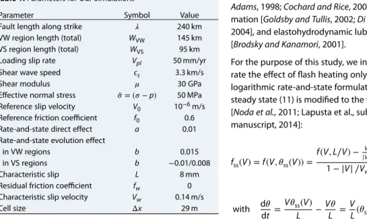
Table 1. Parameters for Our Simulations

Parameter Symbol Value

Fault length along strike _𝜆 240 km VW region length (total) W_VW 145 km VS region length (total) W_VS 95 km Loading slip rate Vpl 50 mm/yr

Shear wave speed c_s 3.3 km/s

Shear modulus _𝜇 30 GPa

Effective normal stress ̄𝜎 = (𝜎 − p) 50 MPa Reference slip velocity V₀ 10−6_m/s

Reference friction coefficient f₀ 0.6 Rate-and-state direct effect a 0.01 Rate-and-state evolution effect

in VW regions b 0.015

in VS regions b −0.01/0.008

Characteristic slip L 8 mm

Residual friction coefficient f_w 0 Characteristic slip velocity V_w 0.14 m/s

Cell size Δx 29 m

materials [e.g., Andrews and Ben-Zion, 1997;

Adams, 1998; Cochard and Rice, 2000], gel

for-mation [Goldsby and Tullis, 2002; Di Toro et al., 2004], and elastohydrodynamic lubrication [Brodsky and Kanamori, 2001].

For the purpose of this study, we incorpo-rate the effect of flash heating only. The logarithmic rate-and-state formulation at steady state (11) is modified to the following [Noda et al., 2011; Lapusta et al., submitted manuscript, 2014]: f_ss(V) = f (V, 𝜃_ss(V)) = f (V, L∕V) − V |V|fw 1 −|V| ∕Vw + V |V|fw, (14) with d𝜃 dt = V𝜃ss(V) L − V𝜃 L = V L(𝜃ss(V) −𝜃), (15) where V_wis the characteristic slip velocity at which flash heating becomes significant (Figure 1b) and f_w is the residual friction coefficient. Based on laboratory experiments and flash heating theories, V_wis of the order of 0.1 m/s. Selecting much larger values of Vwwould effectively disable the additional

weaken-ing due to flash heatweaken-ing, and it would be equivalent to the formulation with the standard but regularized rate-and-state laws (equations (12) and (13)).

2.4. Fault Geometry and Properties

Fault geometry and properties in our simulations have been selected to follow the Kaneko et al. [2010] study for comparison purposes (Figure 1c and Table 1). The fault is therefore 240 km long, subdivided into three VS segments (80 km each on both sides and 15 km in the middle), that surround two VW regions, each 72.5 km long. The length of the central VS segment is varied in our simulations. We assign the rate-and-state param-eter as follows: a is 0.01 for the entire fault, and b varies to define VS and VW areas. The value of b is 0.015 in the VW regions and −0.01 and 0.008 for VS segments on the side and in the middle, respectively. Uniform time-independent effective normal stress (̄𝜎 = (𝜎 − p) = 50 MPa) is applied on the entire fault. The reference slip velocity V0= 10−6m/s, characteristic slip distance L = 8 mm, shear modulus𝜇 = 30 GPa, and shear wave

speed c_s = 3.3 km/s are also constant over the fault. The fault is loaded from the sides by steady motion at the long-term slip rate V_pl = 50 mm/yr. In the case of additional weakening, we set V_wand f_wto be 0.14 m/s and 0, respectively. The weakening is disabled in the VS regions by assigning Vw= 109m/s.

In simulations with the standard rate-and-state law, the shear prestress𝜏₀is equal to that of Kaneko et al. [2010], which is 26.1 MPa for the VS patches on both sides of the fault, 28.2 MPa for the VS patch in the mid-dle, and two different values for the VW areas (28.5 MPa for the left one and 28.8 MPa for the right one), so that nucleation of the first earthquake preferentially starts at one side (right) rather than at the two sides at the same time (Figure 1). In the case of simulations with additional weakening, we apply different𝜏0to

avoid getting large slips in the very first event. Indeed, as discussed in the following, we find that earth-quakes nucleate at lower prestress in the case with additional weakening than in the case with the regular rate-and-state law. Therefore, to be closer to the long-term behavior, the following initial shear stress values have been applied for the cases with enhanced weakening: 23.6 MPa for the VS areas on the sides, 29.4 MPa for the central VS patch, and 9 MPa for the VW segment.

The reference friction coefficient f0is set to be 0.6 everywhere, except for the simulations with additional

weakening, where we use f0to define a nucleation-prone patch. At the boundary between the VS and

VW regions, continuous creep in VS segments concentrates the shear stress, promoting nucleation near these rheological transitions. For simulations with flash heating, we create a 10 km weaker patch next to the boundary between the VS and VW regions, where f₀is decreased to 0.3 (Figure 1a). This weaker patch promotes earlier nucleation and therefore leads to more pulse-like ruptures in FD simulations.

Accumulated slip (m) 10 20 30 40 Fully-Dynamic Model 0 3.56 km/s 0 30 60 90 120 150 180 210 240 10 20 30 40 0

Distance along strike (km)

0 30 60 90 120 150 180 210 240 (a-b) -0.005 0.004 -0.005 0.020 0.020 0.98 km/s Accumulated slip (m) Quasi-Dynamic Model

a

b

Figure 2. Cumulative slip on the fault for (a) FD and (b) QD simulations with the standard rate-and-state law. The slip

is plotted on the fault after the tenth event in both cases. Red lines are plotted every 2 s during seismic events, when the maximum slip velocity exceeds 1 mm/s, while blue lines (every 50 years) illustrate the aseismic behavior of the fault. Black lines represent the cumulative slip after each seismic event. The middle VS patch creates complexity in both FD and QD cases. The FD events are bigger in general, display higher rupture speed (computed between black arrows), and are more likely to rupture the middle VS asperity as discussed in section 5.

3. Simulations of Earthquake Sequences With Standard R&S Law: FD Versus QD

3.1. Fault Response: Common Features

Histories of slip for representative QD and FD simulations with standard rate-and-state law are displayed in Figure 2. The accumulation of slip during interseismic periods is represented by blue lines, which are plot-ted every 50 years. Red lines display cumulative slip every 2 s when the maximum slip velocity on the fault exceeds 1 mm/s, illustrating the end of earthquake nucleation and slip during seismic events.

Despite their relatively simple geometry and distribution of friction properties, the numerical models pro-duce realistic complex fault behavior. They both show seismic and aseismic slip including transients. As expected from stability properties of faults with rate-and-state laws [e.g., Rice and Ruina, 1983], the VS areas are steadily slipping at the slip rate comparable to the plate velocity, whereas VW regions are almost fully locked during interseismic periods and accumulate the slip mainly during seismic events. Earthquakes nucleate where the fault undergoes local stress concentrations due to either rheological transitions from VS to VW regions or arrest of previous earthquakes. Depending on the level of prestress caused by previous slip, some events remain small, rupturing only a fraction of the VW area, while others grow large and propagate through the middle VS barrier. The larger VS regions on both sides of the model act as permanent barriers, and coseismic ruptures penetrate into them only a little. The central VS patch affects rupture propagation, as shown by Kaneko et al. [2010]: sometimes it acts as a barrier, and sometimes coseismic rupture goes through. The behavior depends on a number of factors, as discussed in Kaneko et al. [2010] and section 6. When only one VW segment ruptures, static stress increases at the tip of the previous rupture area, promot-ing propagation of the subsequent event through the VS patch, and it leads to the stress transfer into the neighboring VW segment. This often leads to the nucleation of another event, shortly after the first one, at the boundary between the central VS patch and the unruptured VW area, which is a type of clustering.

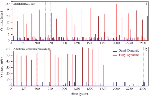
0 10 Vs max (m/s) 5 15 20 30 25

a

Standard R&S law

0 20 Vs max (m/s) time (year) 1250 500 1750 2500 250 1000 1500 2000 10 30 40 750 2250 60 50 0 1250 500 1750 2500 250 750 1000 1500 2000 2250 0 Quasi-Dynamic Fully-Dynamic

b

Additional coseismic weakening

Figure 3. The maximum slip velocity over the fault for the QD and FD simulations (a) without and (b) with additional

coseismic weakening for the reference cases plotted in Figures 2 and 5, respectively. In both cases, the maximum velocity is much higher (about 10 times) in the FD simulations than in the QD ones. Accounting for additional coseismic weaken-ing also increases significantly the slip velocity (about 2 times) for both QD and FD formulations, but the ratio between the two stays similar. The vertical dashed lines illustrate the time limit for which we plot the cumulative slip on the fault in Figures 2 and 5.

3.2. QD Versus FD: Differences

The QD and FD simulations also exhibit important quantitative and qualitative differences. The first observa-tion is that the final slip is smaller in the QD case than for the FD simulaobserva-tion. As a consequence, fewer events are needed in the FD case to accumulate the same amount of slip. Furthermore, the rupture speed and slip velocity, which are indicated by the horizontal and vertical spacing of red lines, respectively, are much lower for the QD simulation than for the FD one. If we compute the average rupture speed between black arrows in Figure 2, we find 3.56 km/s and 0.98 km/s for the FD and QD simulations, respectively. This phenomenon is

16 20

shear stress (MPA)

18 22 24 30 28 26 time (year) 1250 500 1750 2500 250 750 1000 1500 2000 2250 0

Figure 4. Spatially averaged shear stress on the fault (𝜏av) over many earthquake cycles computed from equation (16).

The solid curves correspond to the QD (blue) and FD (red) standard rate-and-state (R&S) simulations. The correspond-ing vertical lines show the time limit for which we plot accumulation of slip on the fault in Figure 2. The dashed lines represent the stress levels for the QD (blue) and FD (red) simulations with additional coseismic weakening. Similarly, the corresponding vertical lines show the time over which we plot cumulative slip in Figure 5. The grey line gives a represen-tative fault-averaged quasi-static fault strength (_̄𝜎f0). In both cases (FD and QD), for the standard R&S law simulations, the average fault prestress before large, fault-spanning events is close to the representative static fault strength. In con-trast, when models account for flash heating, the average fault prestress is significantly below the static fault strength, particularly for the FD case.

also illustrated in Figure 3a, which displays the maximum sliding velocity recorded during one event. These differences have already been pointed out by Lapusta et al. [2000] and Lapusta and Liu [2009].

To quantify the evolution of the stress state on the fault for the two models, we consider the average shear stress𝜏_av(t), defined as follows:

𝜏av(t) = 1 z2− z1∫ z2 z1 𝜏(z, t)dz, (16)

where the spatial integration is taken over the velocity-weakening regions plus the central patch, excluding the VS areas on the sides. Therefore, z1 = 40 km and z2 = 200 km for the two examples shown in Figure 2

(see Figure 1 for fault geometry). The time evolution of the average stress for the standard rate-and-state laws is plotted in Figure 4 with solid curves. The vertical solid lines correspond to the time limit for which the accumulation of slip on the fault is shown in Figure 2. The variations in the average shear stress display steady interseismic accumulation of stress due to the tectonic loading, with occasional abrupt drops rep-resenting the simulated earthquakes. Consequently, local peaks of the average shear stress correspond to the level of stress on the fault before earthquakes nucleate. For both curves, the peaks are close to the rep-resentative quasi-static (or low-velocity) fault strength̄𝜎f₀ = 30 MPa (the grey line in Figure 4) averaged over the seismogenic part of the fault (VW segments + VS asperity), but the FD simulation displays a slightly smaller value compared to the QD model. This shows that the FD formulation promotes the nucleation, with the wave-mediated stress transfer enhancing the stress concentration in the nucleation zone and promot-ing the transition to rapid expansion at lower values of prestress. If one divides the shear stress peak values by the effective normal stress (50 MPa) to estimate the equivalent friction coefficient, one finds a value of

0.55 for the QD simulation and 0.54 for the FD case, which is close to the representative quasi-static friction

coefficient (f₀ = 0.6). The stress drop for the larger events is, on average, ∼ 0.99MPa and ∼ 1.26MPa for the QD and the FD simulations, respectively, which is consistent with the difference in the cumulative slip per event observed in Figure 2. Note that we estimate the stress drop directly from the fault-averaged shear stress change from Figure 4. Such fault-averaged stress is not exactly equal to the seismologically estimated moment-based stress drop [Noda and Lapusta, 2013]. However, for the relatively uniform slips that we have in our models, the two estimates are quite close.

Overall, the FD and QD models in the case of standard rate-and-state law are qualitatively similar but quan-titatively different. We will see in the following section that the differences are much more dramatic in the presence of enhanced coseismic weakening.

It has been hypothesized [Lapusta et al., 2000] that smaller radiation damping terms in the QD formulation can make the comparison with FD models more favorable. In that case, constant𝛽_sis added to equation (1):

𝜏(z, t) = 𝜏0_{(z, t) + 𝜙(z, t) −} 𝜇

2cs𝛽s

V(z, t), (17)

with𝛽s ≥ 1. Lapusta and Liu [2009] have explored this hypothesis for 3-D cases and found that indeed,

the rupture speed in the QD simulations increases with the higher values of𝛽s; however, the slip

veloc-ity remains small in comparison with the FD events. Moreover, final slip, average slip per event, and static stress drop are smaller for all the QD simulations they have explored (𝛽s =1, 2 or 4). Lapusta and

Liu [2009] also emphasized that increasing𝛽sfurther is not a promising approach, since the rupture

speed for𝛽s = 4 is already higher than that in the FD case. Therefore, the QD approach can be used to

explore the fault behavior qualitatively in some cases (see section 7 for more discussion), but it cannot be precise quantitatively.

4. Simulations of Earthquake Sequences With Additional Weakening: FD Versus QD

4.1. Fault Response: Seismic and Aseismic Slip, Including Transient

Despite having the same model parameters, QD and FD simulations display drastic differences in cases with additional dynamic weakening. Slip history for representative QD and FD simulations is displayed in Figure 5. As for Figure 2, the accumulation of slip during the interseismic period is plotted every 50 years in blue, whereas the accumulation of slip during seismic events is displayed every 2 s with red lines. For plot-ting purposes, we increase 4 times the ordinate axis for the QD simulation, but we keep the same scale as in

0 40 80 120 160 24 Accumulated slip (m) 10 20 30 40 Fully-Dynamic Model 0 0 30 60 90 120 150 180 210 240 0 30 60 90 120 150 180 210 240

Distance along strike (km)

(a-b) -0.005 0.004 -0.005 0.020 0.020 Accumulated slip (m) Quasi-Dynamic Model 19 ! x4 bigger scale

a

_{every 50 years} every 2 s

b

Figure 5. Cumulative slip on the fault for the (a) FD and (b) QD simulations with the rate-and-state law and

addi-tional coseismic weakening. The slip is plotted on the fault after the after the third and the eighteenth events in the QD and the FD cases, respectively. Note that theyaxis has 4 times larger values in Figure 5b than in Figure 5a. Red lines are plotted every 2 s during seismic events, while blue lines are plotted every 50 years. Black lines represent the cumulative slip after each seismic event. Grey shading represents the spatial extent of the fault slipping during a rep-resentative 2 s interval. The FD and QD events are very different in size, recurrence, and propagation mode. The FD solution generates pulse-like events, while the QD formulation results in smaller events in the form of dying pulses and large crack-like events. The slip-rate snapshots for events 19 in Figure 5a and 24 in Figure 5b are displayed in Figures 6 and 7, respectively.

Figure 2 for the FD case. Both FD and QD simulations show seismic and aseismic slip, including transients, but earthquake ruptures are very different in size, recurrence, and propagation mode.

The first observation is that earthquake events in the QD simulations are quite different from the ones in the FD simulations if the friction law includes coseismic weakening mechanisms. For example, event 24 in the QD model (Figure 5) displays a maximum slip of 75 m, while FD simulations record ∼6m of slip on average, with the peak at 7 m. Moreover, despite the simple geometry and the same parametrization, QD simulations produce a more complex earthquake sequence behavior. In the FD model, for this particular setup, all events are able to propagate through the VS region in the middle and look very similar to one another. In the QD solution, depending on the level of prestress, some events remain small, rupturing only a fraction of the VW area, while others grow large and propagate through the middle VS barrier (Figure 5).

4.2. Pulse-Like Ruptures in FD Versus Crack-Like Ruptures in QD Simulations

The mode of rupture for the largest events in the two simulations are radically different: the FD solution gen-erates pulse-like events, while the QD formulation results in crack-like events. To illustrate this phenomenon, Figure 5 shows in grey the spatial extend of fault slipping during a 2 s interval, close to the end of the rup-ture. For event 19 in the FD simulation, only a small part of the fault (∼ 10 km out of 160 km) slips during those 2 s, while in the QD simulation (event 24), the slipping area is 140 km out of 160 km, with most of the seismogenic part of the fault slipping. We see that for the QD cases, the region where the earthquake nucleated keeps slipping as the rupture propagates further.

120 30 60 90 150 180 120 30 60 90 150 180 30 60 90 120 150 180 210 0 t = 48 s t = 44 s t = 40 s t = 36 s t = 16 s 20 30 10 t = 12 s 0 20 30 10 t = 8 s 0 20 30 10 t = 4 s 0 20 30 10 40 t = 28 s 0 20 30 10 t = 32 s 20 30 10 t = 20 s 0 20 30 10 t = 24 s 20 30 10 0 0 20 30 10 20 30 10 0 20 30 10 20 30 10 0 slip rate (m.s-1)

Figure 6. Snapshots of slip rate on the fault for a representative FD event with enhanced coseismic weakening. The

slip rate is nonzero only on a small portion of the fault at a time, indicating that the rupture propagates as a narrow self-healing slip pulse (which is actually a double pulse in most snapshots). The slip rate increases as the rupture prop-agates through the first (right) VW segment, but then decreases when the rupture encounters the VS middle patch. Propagation in the second VW patch leads to the slip rate increasing again. For the cumulative slip history of this seismic event (number 19), see Figure 5.

Evolution of slip rate through time for the two events is another way to emphasize the difference (Figure 6 for FD event 19 and Figure 7 for QD event 24). Both seismic events nucleate similarly, but thereafter they dis-play a very different story. In the FD dynamic case (Figure 6), while propagating through the VW area, the slipping region is consistently narrow, and the second pulse is developed (t = 8 s to t = 29 s). When the rupture encounters the central VS patch (t = 28 s), the slip rate drastically decreases. Propagation in the second VW patch leads again to the creation of a double pulse, and the slip rate increases up to 40 m/s. For

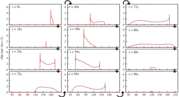
t = 8s 0 4 6 2 t = 16s 0 4 6 2 t = 24s 0 4 6 2 t = 32s 4 6 2 t = 72s t = 80s t = 88s t = 96s t = 40s t = 56s t = 64s t = 48s 120 30 60 90 150 180 120 30 60 90 150 180 30 60 90 120 150 180 210 0 0 4 6 2 0 4 6 2 0 4 6 2 4 6 2 0 4 6 2 0 4 6 2 0 4 6 2 4 6 2 slip rate (m.s-1)

Figure 7. Snapshots of slip rate on the fault for a representative model-spanning QD event with enhanced coseismic

weakening. As the rupture propagates through the fault, segments that have already sustained seismic motion still accu-mulate more slip, which leads to the development of a crack-like rupture. The middle VS patch decreases the slip rate but does not stop the rupture. For the cumulative slip history of this seismic event (number 24), see Figure 5.

QD event number 24 (Figure 7), nucleation starts within the right VW region, and then the rupture extends bilaterally in a crack-like mode. The rupture becomes less vigorous as it propagates through the central VS patch and then resurges on the other side, with large slips that promote the rerupturing of the right VW patch.

Note that the smaller events in the QD case, the ones that nucleate at the sides of the seismogenic region and arrest before reaching the middle of the fault, propagate as dying pulses.

4.3. Average Shear Stress Level on the Fault

The state of stress on the fault is strongly influenced by the FD versus QD modeling procedures. The time evolution of average shear stress (equation (16)) for the QD and FD models with additional weakening mechanisms is plotted in Figure 4 with dashed blue and red curves, respectively. The corresponding verti-cal lines show the time limit for which the accumulation of slip is illustrated (Figure 5). Unlike for simulations that assume the standard rate-and-state logarithmic-type coseismic weakening, the average shear stress on the fault with additional coseismic weakening is much smaller than the quasi-static strength̄𝜎f0. Accounting

for full inertial effects further reduces the average stress level. In the simulation with additional weakening and wave-mediated stress transfers (dashed red curves), the peaks of the average shear stress are between 16.5 and 17.3 MPa, with the equivalent friction coefficients of 0.33 and 0.35, respectively. The seismic events are very similar, with the return period of ∼ 92 years on average and a stress drop of ∼0.78 MPa. The QD simulation displays a very different behavior. Interseismic increase of average shear stress, punctuated by stress drop due to smaller events, is observed over a period of ∼1100 years until the stress reaches a peak of 23.6 MPa. During that time, smaller events can occur on the sides of the fault, and their stress drops appear smaller on this plot due to averaging over the entire fault. The equivalent coefficient of friction in this QD case is close to 0.47. Thereafter, the fault records a large event with the stress drop of 6.5 MPa, 8.3 times bigger than that of a representative FD event (Figure 4).

5. Reasons for the Dramatic Differences Between FD and QD Simulations With

Enhanced Weakening

It is clear that the QD simulations produce qualitatively different outcomes from the FD ones in the cases with enhanced coseismic weakening, unlike our findings for the models with standard rate-and-state weak-ening only, as in section 3. In all cases, the exclusion of the wave-mediated stress transfers lowers stress concentration at the rupture tip, hence lowering slip rates there. In the case of the standard rate-and-state law, this mostly leads to slower rupture speeds, consistent with dynamic fracture mechanics [e.g., Freund, 1990]; however, the amount of weakening the fault experiences is virtually unchanged, since the weak-ening in the standard rate-and-state friction laws is only logarithmically dependent on the slip rate. In the case of enhanced coseismic weakening, however, the dependence of fault weakening on the slip rates is much stronger, and the reduction of slip rates in the QD simulations has a profound effect on how the fault weakens with slip. In essence, the FD simulations have more intense fault weakening than the QD ones, promoting low-stress fault operation and pulse-like rupture mode, as consistent with previous numeri-cal findings [Zheng and Rice, 1998; Noda et al., 2009, 2011; Lapusta et al., submitted manuscript, 2014]. As a result, the FD simulations have the fault operating under low overall prestress (section 4.3) with all ruptures propagating in the pulse-like mode (section 4.2), while the QD simulations produce a mixture of smaller events that arrest as dying pulses and much larger, model-spanning, crack-like ruptures under larger prestress.

The differences between the FD and QD simulations manifest themselves even during the nucleation pro-cesses. As mentioned in section 2.4, for the simulations with additional weakening, the reference friction coefficient f0is defined to be 0.6 everywhere, except for the nucleation-prone patch near the transition zone

between the VW and VS segments (at x ≃ 45 km in Figure 1). In the FD models, all events nucleate at that particular location. In the QD simulations, events nucleate on both sides of the VW fault and even at the boundary with the VS barrier in the middle of the fault (Figure 5), while the weaker patch simply produces more numerous small events. This can be linked to the level of stress at which events are able to propagate, which varies in the two models. In both cases, earthquakes can nucleate in the nucleation-prone patch while most of the fault is far from its static strength. By the time the rupture reaches the statically stronger parts of the faults (where f0 = 0.6), it must be able to cope with the high mismatch between the prestress and the

slip rates and their associated greater weakening, but not in the QD simulations, which can only support the dying pulse-like and the crack-like mode. This is why we observe the interseismic average stress increases over a period of ∼1100 years in the QD simulation (Figure 4), which brings the VW segments to a stress level closer to its quasi-static strength value.

6. Quantifying the Effect of VS Patches on Seismic Ruptures

As mentioned in section 1, an important question in seismotectonics is the ability of the earthquake rupture to propagate over faults with heterogeneous properties. In particular, a case of seismogenic patches sepa-rated by creeping barriers has emerged as one of significant practical interest, based on observations [e.g.,

Burgmann et al., 2005; Hetland and Hager, 2006; Chlieh et al., 2008; Perfettini et al., 2010; Chlieh et al., 2011; Loveless and Meade, 2011]. Kaneko et al. [2010] explored the dependence of earthquake rupture patterns

and interseismic coupling on spatial variations of fault friction using FD simulations. Here we consider the importance of accounting for full wave-mediated effects in modeling of that kind.

Following the study of Kaneko et al. [2010], we analyze the probability P of an earthquake to rupture the VS middle patch in QD dynamic simulations to compare with the statistics computed for FD models. We start each simulation with arbitrary initial conditions (described in subsection 2.4) and then simulate the fault behavior for 10,000 years. Based on the study of Kaneko et al. [2010], the probability P is estimated from the percentage of earthquakes that propagate through the VS patch relative to the number of earthquakes that rupture entirely one or two of the VW segments [Kaneko et al., 2010]. Kaneko et al. [2010] identified a nondimensional parameter, B, which correlates with the probability P. The parameter B relates the amount of stress that is needed by the VS patch to sustain the rupture and the amount of stress that the incoming rupture can provide to the VS patch. It is given by

B = Δ𝜏propDvs

𝛽Δ𝜏vwDvw

, (18)

which can be approximated as

B ≃ln(V

dyn

vs ∕Vvsi )̄𝜎vs(avs− bvs)Dvs

𝛽Δ𝜏vwDvw

, (19)

where Δ𝜏_propis the stress required by the VS patch; D_vsand D_vware the sizes of the VS patch and VW seg-ment, respectively; Δ𝜏_vwis the average coseismic stress drop over the VW segment from which the rupture is attempting to enter the VS patch;̄𝜎vsis the normal stress in the VS patch; V

dyn

vs and Vvsi are the seismic and

preevent (interseismic) velocity in the VS patch, respectively; avs−bvs>0 is the velocity-strengthening

param-eter in the VS patch; and𝛽 is a model-dependent geometric factor that specifies the fraction of the stress transferred onto the VS patch; following Kaneko et al. [2010], we use𝛽 = 0.5 for the 2-D model considered here. As B increases from 0 to ∼1, the percentage P drops from 100% to 0% [Kaneko et al., 2010].

6.1. Models With Standard Rate-and-State Friction

For simulations with the standard rate-and-state law, the dependence of the propagation probability P on the parameters of the VS patch displays similar trends in the FD and QD simulations (Figures 8a and 8b). For both approaches, the higher the value of (avs− bvs) and/or the larger the size Dvs, the more efficient the

patch is in stopping earthquake rupture, which is consistent with the prediction based on the parameter B. Moreover, if we look at the distributions of slip in individual events (cases Q1–3 and F1–3 in Figure 9), the overall rupture pattern is qualitatively similar.

Nevertheless, there are important quantitative differences. In the QD simulations, the VS patch acts as a permanent barrier for smaller values of (a_vs− b_vs) and/or D_vs(Figure 8a) than in the FD simulations. Further-more, for most cases in which the VS patch is a partial barrier, up to 30% more events propagate through the VS patch in the FD simulations that incorporate full inertial effects (Figure 8c). These results are likely due to two factors. First, the stress drop (Δ𝜏vw) in equation (18) is higher for the FD simulations (Figure 4 and

section 3.2), leading to smaller B and hence higher probability of propagation P. Second, incorporating all wave-mediated stress transfers—as in the FD simulations—leads to higher stress concentration at and in front of the rupture tip and hence promotes rupture propagation through unfavorable regions such as the VS patch. This latter effect is not completely accounted for by parameter B, which is based on quasi-static consideration of stress transfer.

0 10 20 30 40 50 60 VS patch size, D (km) 0 0.002 0.004 0.006 0.008 0.010 0 0.002 0.004 0.006 0.008 0.010

a

b

0 0.002 0.004 0.006 0.008 0.010

c

0 0.001

d

0 0.001

e

0 10 20 30 40 50 60 0 20 40 60 80 100

Figure 8. The ability of seismic ruptures to propagate through an unfavorable fault region in the form of a VS patch in

simulations with the rate-and-state friction only. The relation between the properties of the VS patch and the probability

P(in color) that an earthquake would propagate through it is shown for the (a) QD approach (this study) and (b) FD approach (modified from [Kaneko et al., 2010]). Each colored dot corresponds to a 10,000 year simulation of fault slip with more than 50 events that rupture either one or both VW segments.P = 0% means that the VS patch is a permanent barrier. Black lines are the isocontours ofP. Slip distributions in seismic events for cases Q1–3 and F1–3 are displayed in Figure 9. (c) The difference in probabilityPbetween the QD and FD cases. (d) Several FD simulations recomputed with the same code and computational cluster as the QD simulations (see the text for more explanation). (e) The difference in probabilityPbetween the QD and FD cases from Figure 8d.

Note that in the particular case of a velocity-neutral patch ((avs− bvs) = 0) and for another case where the

velocity strengthening of the patch is small ((a_vs− b_vs) = 0.001, D_vs= 5 km), we observe the opposite trend: the QD formulation seems to slightly enhance rupture propagation through the patch (Figure 8c). Since our QD computations (Figure 8a) have been executed on a different computational cluster and with an updated

Quasi-dynamic Model

Distance along strike (km)

0 5 10 15

Q2

Distance along strike (km)

0 5 10 15 Q3 0 60 120 180 240 0 60 120 180 240 0 60 120 180 240 0 60 120 180 240 0 60 120 180 240 0 60 120 180 240 0 5 10 Slip (m) Q1

Distance along strike (km)

Distance along strike (km) Distance along strike (km) Distance along strike (km)

(This study)

5

Fully-dynamic Model

0 (Modified from Kaneko et al., 2010)

0 5 10 15 Slip (m) F1 0 5 10 15 F2 10 15 F3

(%) of EQ going through VS patch 0 20 40 60 80 100

Figure 9. Slip distributions of the seismic events corresponding to cases Q1–3 (QD simulations) and F1–3 (FD

simula-tions) from Figure 8, illustrating the range of fault behaviors that both QD and FD simulations can produce, but not for the same properties of the VS region. The VS patch can either act as a permanent barrier (Q1 and F1) or let some of the earthquakes propagate through (Q2–3 and F2–3).

0.001 0.002 0.003 0.004 0.005 0.006 0.007 0.008 0.009 0.01 0 10 20 30 40 50 60 70 80 90 100 a b c 0 5 10 0 30 60 90 120 150 180 210 240 0 30 60 90 120 150 180 210 240 0.006 0.020 0.020 0 20 10 30

Figure 10. The ability of seismic ruptures to propagate through an unfavorable fault region in the form of a VS patch in

simulations with additional coseismic weakening. (a) The probabilityPthat an earthquake propagates through a 15 km patch is plotted against the friction parameter(a − b)of the patch. Each red square corresponds to a 10,000 year FD simulation of fault slip with more than 50 events that rupture either one or both VW segments. Events spanning the entire fault are more rare with the QD simulations (blue dots); therefore, the QD statistics have been computed over at least 20 events that arrest at or propagate through the VS patch. The FD and QD results are quite different, as discussed in the text. (b and c) Cumulative slip on the fault for representative events in the FD and QD simulations, respectively, when(a_vs−b_vs) = 0.006. Red lines are plotted every 2 s during seismic events, while blue lines are plotted every 50 years.

code compared to the FD simulations of Kaneko et al. [2010], we first check whether there might be small computational differences between the two types of simulations. To that end, we redo the FD computa-tions for the cases in question (Figure 8d) and indeed find that the results are slightly different, by 0 to 5% in the propagation probability P. This is not surprising, since small differences in the order of the computa-tional operations accumulate and can lead to rupture arrest or propagation over the VS patch in these highly nonlinear problems. Comparing the FD and QD calculations done with the same code on the same com-putational cluster, we still find that the QD simulations lead to slightly more ruptures propagating through the VS patch in some cases (e.g., (avs− bvs) = 0, Dvs = 10 km), although the difference is smaller, up to

at most 5% (Figure 8e), while for some other cases (e.g., (avs− bvs) = 0, Dvs = 15 km), the FD simulations

now have a slight edge of up to 0.5%. Overall, these results imply that the difference between FD and QD simulations for rupture propagation over the velocity-neutral patch is near 0. This is consistent with our sim-ulations without the patch, where large events, once they reach the middle of the fault, propagate to the other end of the fault in both FD and QD simulations, implying 100% propagation probability (recall that P is computed based only on those events that fully rupture one of the VW sides of the fault). The addition of a patch with properties close to the rest of the fault cannot change this behavior much, at least for relatively small patches, and the FD and QD simulations both have near-100% probability of propagation through the patch in those cases.

Overall, the effect of FD versus QD simulations with the standard rate-and-state friction on the ability of rupture to propagate through an unfavorable patch is similar to the comparison discussed in section 3: the results are qualitatively similar but quantitatively different.

6.2. Models With Enhanced Coseismic Weakening

For the models with enhanced coseismic weakening, we explore a smaller representative subset of cases to shorten the computational time. We consider a 15 km long VS patch with a range of velocity-strengthening (avs− bvs) values (Figure 10a).

As expected, based on the results of section 4, the two simulation approaches display more dramatic dif-ferences in the models with enhanced coseismic weakening. For small values of (a_vs− b_vs), almost 100% of the large events propagate through the middle patch, in both cases, as in the models with the standard rate-and-state friction (section 6.1). However, the behavior deviates for larger values of (a_vs− b_vs). In the QD cases, the decrease in probability P is essentially gradual with (a_vs− b_vs) and relatively slow, with about 50% of ruptures propagating through the VS patch for the largest value, 0.01, of (a_vs− b_vs) explored. In the FD case, near-100% propagation persists until (a_vs− b_vs)≤ 0.005, and then the propagation probability P relatively rapidly drops, with the VS patch essentially becoming a permanent barrier for (a_vs− b_vs)≥ 0.008. The differences between the rupture-patch interaction in the FD and QD simulations can be explained by the differences in the rupture propagation mode and size detailed in section 4. The FD simulations produce similar pulse-like ruptures that initiate on the side of the VW segment away from the patch and attempt to propagate over the patch after entirely rupturing one of the VW segments (e.g., Figures 5 and 10b). Such behavior results in a relatively stable value of Δ𝜏vw, of about 3 MPa in our cases. Using this value in

the approximate expression of B, equation (19), with the typical value of ln(Vvsdyn∕Vvsi ) = 20 [Kaneko et al.,

2010], and determining the value of (avs− bvs) that corresponds to B = 1 results in 0.007. The value of

(a_vs− b_vs) = 0.007 is indeed close to the value of 0.008, at which point the VS patch becomes a permanent barrier in the fully dynamic case (Figure 10). The decay of the probability over a range of (avs− bvs) values,

from 0.005 to 0.008, is likely related to the variability of events and interevent times—and hence values of Δ𝜏_vwand Vi

vs—observed in the FD simulations (Figures 5a and 4).

In the QD simulations, the larger events that attempt to break the VS patch nucleate at different distances from the VS patch, including right next to it, and hence they are in a different state of their development when they reach the VS patch. This results in different relevant values of Δ𝜏_vwand effective ruptured D_vw (Figure 10c, where the relevant region is shaded) and hence complexifies the application of equations (18) and (19) for B to this case. Furthermore, many of the events that cross the VS patch occur right after other attempts, benefiting from elevated slip rate and stress on the VS patch from the previous attempt (as in Figure 10c), which significantly affects the slip rate Vi

vsin equation (19). However, the expression for the

parameter B is still helpful in understanding why the QD simulations in the models with enhanced weak-ening are more likely to result in rupture propagation over the VS patch than the FD simulations. This is because the largest events that attempt to propagate over the patch have much larger values of Δ𝜏vwin the

QD simulations than in the FD simulations, up to a factor of 8 in the case considered in section 4.

Overall, the ability of the rupture to propagate over the VS patch is significantly affected by the FD versus QD simulations in the models with enhanced dynamic weakening, as expected based on the significant differ-ences between the simulations documented in section 4. Furthermore, the effect is not intuitive. One might intuitively think that the FD ruptures would be more likely to propagate through the patch, as observed in the cases with the standard rate-and-state friction, but this is not true in these models, since the QD simula-tions result in crack-like ruptures with much larger slip and stress drops than for the FD reference case and hence have a significant edge in terms of their ability to propagate through the patch.

7. Conclusions

We have investigated the differences between the fully dynamic (FD) simulations that properly incorpo-rate the wave-mediated stress transfers and the quasi-dynamic (QD) simulations that ignore the transient nature of the stress transfers. The results demonstrate that the QD simulations can be qualitatively very dif-ferent from the FD simulations in situations where the wave-mediated stress transfers significantly affect the model response.

In the models with the standard rate-and-state friction and relatively uniform fault properties (section 3), the FD and QD simulations produce qualitatively similar fault behaviors, with crack-like ruptures and similar earthquake patterns. There are, however, quantitative differences, with the FD simulations having frac-tionally larger amounts of slip per event, correspondingly larger stress drops, and significantly higher slip velocities and rupture speeds. These findings are similar to those of previous studies with similar models [Lapusta et al., 2000; Lapusta and Liu, 2009]. In terms of the ability of the rupture to propagate over unfa-vorable patches, for example, due to their VS friction properties as considered in this study, the trends with respect to the patch parameters are similar in the FD and QD simulations, but the events in the FD

simula-tions are more likely to propagate over the patch for most cases considered. This is due to the higher stress drop in the FD simulations, which is an important parameter based on the study of Kaneko et al. [2010], as well as higher slip rates and hence more pronounced dynamic stress concentration.

However, the results of the FD and QD simulations become qualitatively different for the models with enhanced dynamic weakening, where the wave-mediated stress changes contribute to the formation of self-healing slip pulses [Zheng and Rice, 1998]. In that case, the FD simulations produce pulse-like ruptures that nucleate at the prescribed weaker site, whereas the QD simulations produce numerous smaller events at the edges of the seismogenic part of the model, until a much larger crack-like event spans the entire seismogenic part of the fault. The largest events in the QD simulations have much larger average slip and stress drop than the largest FD events, up to a factor of 8 in our simulations. This finding is a clear reversal of what is observed in models with the standard rate-and-state friction, where the FD events are larger in slip and stress drop. Similarly to the models with the standard rate-and-state friction, the slip rate and rupture speed is significantly higher in the FD simulations with enhanced coseismic weakening than in the QD ones. However, unlike in the models with the standard rate-and-state friction, where the coseismic fault resistance is minimally affected, the higher slip rates in the models with enhanced coseismic weakening result in more pronounced fault weakening and hence substantially change the fault behavior. In part, the average shear stress on the fault is significantly lower in the FD simulations, including before the largest model-spanning events, leading to self-healing pulse-like ruptures [Zheng and Rice, 1998; Noda et al., 2009]. As a result of their much larger slip and stress drop, the large events in the QD simulations are more likely to propagate through the unfavorable fault patch, again contrary to the models with the standard rate-and-state friction. The inability of the QD simulations to produce sustained self-healing pulse-like events is a serious limita-tion, as seismological observations show that this is the most common mode of earthquake rupture [e.g.,

Heaton, 1990].

We expect similarly dramatic differences between the FD and QD simulations in other cases where wave-mediated transient effects can lead to qualitative differences. One such case is the rupture tran-sition to supershear speeds [e.g., Andrews, 1976; Xia et al., 2004; Liu and Lapusta, 2008], in which the wave-mediated stress transfers either produce a secondary supershear rupture ahead of the main one [Andrews, 1976] or induce the main rupture front to jump to the supershear speeds [Liu and Lapusta, 2008]. Another case is that of strong local heterogeneities that can produce local arrest waves and cause short local rise time [e.g., Beroza and Mikumo, 1996], a phenomenon that may not be captured by the QD simulations. Considering both models, we find that ignoring the transient wave-mediated stress transfers, which are a significant part of inertial effects, may lead to (1) misprediction of the size and recurrence of earth-quakes, (2) incorrect average stress levels on the fault, and (3) missed characteristic features such as the sustained pulse-like mode of rupture propagation. Note that even the postseismic slip may be significantly affected, due to the differences in the coseismic rupture and its interaction with the potentially creeping VS fault areas.

This study has concentrated on 2-D models, for numerical feasibility. However, we expect that 3-D model-ing would yield qualitatively similar results. Comparisons between QD and FD simulations for 3-D models with a regular rate-and-state law were performed by Lapusta and Liu [2009]. They show that the QD approach modifies long-term slip patterns in addition to resulting in much smaller slip velocities and rupture speeds during dynamic events, much as we observe for the 2-D cases. Earthquake sequence sim-ulations in 3-D models with flash heating are quite expensive computationally and consequently have not been done. However, we expect 3-D simulations to give quite similar results. Indeed, self-healing pulse-like ruptures—which give rise to the dramatic differences between the QD and FD results in this study—have been observed in 3-D simulations of earthquake sequences with thermal pressurization [Noda and Lapusta, 2010]. We can therefore speculate that the 2-D results presented here are qualitatively applicable to 3-D models.

We conclude that in order to correctly interpret observations of individual earthquakes and the entire fault slip cycle, or to draw inferences regarding fault friction, it is important to use the right modeling approach. Under certain conditions, such as the standard rate-and-state friction and relatively homogeneous faults with no possibility of supershear transition, the QD simulations could be appropriate. However, since it is dif-ficult to predict the outcome of the FD simulations, and hence the presence or absence of certain features, it is important to verify the results with the FD approach at least for some representative cases.