HAL Id: hal-00296398
https://hal.archives-ouvertes.fr/hal-00296398
Submitted on 12 Dec 2007
HAL is a multi-disciplinary open access
archive for the deposit and dissemination of
sci-entific research documents, whether they are
pub-lished or not. The documents may come from
teaching and research institutions in France or
abroad, or from public or private research centers.
L’archive ouverte pluridisciplinaire HAL, est
destinée au dépôt et à la diffusion de documents
scientifiques de niveau recherche, publiés ou non,
émanant des établissements d’enseignement et de
recherche français ou étrangers, des laboratoires
publics ou privés.
cluster analysis of observations and model results
O. A. Tarasova, C. A. M. Brenninkmeijer, P. Jöckel, A. M. Zvyagintsev, G. I.
Kuznetsov
To cite this version:
O. A. Tarasova, C. A. M. Brenninkmeijer, P. Jöckel, A. M. Zvyagintsev, G. I. Kuznetsov. A climatology
of surface ozone in the extra tropics: cluster analysis of observations and model results. Atmospheric
Chemistry and Physics, European Geosciences Union, 2007, 7 (24), pp.6099-6117. �hal-00296398�
www.atmos-chem-phys.net/7/6099/2007/ © Author(s) 2007. This work is licensed under a Creative Commons License.
Chemistry
and Physics
A climatology of surface ozone in the extra tropics: cluster analysis
of observations and model results
O. A. Tarasova1,2, C. A. M. Brenninkmeijer1, P. J¨ockel1, A. M. Zvyagintsev3, and G. I. Kuznetsov2
1Max Planck Institute for Chemistry, Mainz, Germany
2Lomonosov Moscow State University, Faculty of Physics, Moscow, Russia
3Central Aerological Observatory, Dolgoprudny, Russia
Received: 6 July 2007 – Published in Atmos. Chem. Phys. Discuss.: 23 August 2007
Revised: 14 November 2007 – Accepted: 20 November 2007 – Published: 12 December 2007
Abstract. Important aspects of the seasonal variations of
surface ozone are discussed. The underlying analysis is
based on the long-term (1990–2004) ozone records of the Co-operative Programme for Monitoring and Evaluation of the Long-range Transmission of Air Pollutants in Europe (EMEP) and the World Data Centre of Greenhouse Gases, which provide data mostly for the Northern Hemisphere. Seasonal variations are pronounced at most of the 114 lo-cations at all times of the day. A seasonal-diurnal varia-tions classification using hierarchical agglomeration cluster-ing reveals 6 distinct clusters: clean background, rural, semi-polluted non-elevated, semi-semi-polluted semi-elevated, elevated and polar/remote marine. For the “clean background” clus-ter the seasonal maximum is observed in March-April, both for night and day. For those sites with a double maximum or a wide spring-summer maximum, the spring maximum ap-pears both for day and night, while the summer maximum is more pronounced for daytime and hence can be attributed to photochemical processes. The spring maximum is more likely caused by dynamical/transport processes than by pho-tochemistry as it is observed in spring for all times of the day. We compare the identified clusters with correspond-ing data from the 3-D atmospheric chemistry general cir-culation model ECHAM5/MESSy1 covering the period of 1998–2005. For the model output as for the measurements 6 clusters are considered. The simulation shows at most of the sites a spring seasonal maximum or a broad spring-summer maximum (with higher summer mixing ratios). For southern hemispheric and polar remote locations the seasonal maxi-mum in the simulation is shifted to spring, while the absolute mixing ratios are in good agreement with the measurements. The seasonality in the model cluster covering background locations is characterized by a pronounced spring (April– May) maximum. For the model clusters which cover rural Correspondence to: O. A. Tarasova
and semi-polluted sites the role of the photochemical pro-duction/destruction seems to be overestimated. Taking into consideration the differences in the data sampling procedure, the comparison demonstrates the ability of the model to re-produce the main regimes of surface ozone variations quite well.
1 Introduction
Ozone is a key species of tropospheric chemistry, polluted or pristine (Crutzen, 1973; Fabian and Pruchniewz, 1977), and it is a greenhouse gas (IPCC, 2006). Surface ozone is of special concern as an air pollutant. Particularly, despite the measures taken to ameliorate surface ozone increase by re-ducing precursor emissions (Ord´o˜nez et al., 2005; Vingarzan, 2004; Oltmans et al., 2006), its level appears to be increas-ing. Jonson et al. (2006) suggested that reductions in regional ozone production were annulled by increasing levels of back-ground ozone, thus leading to the upward trend observed at Mace Head in Ireland. A possible explanation of the posi-tive trend at the elevated European sites has been proposed by Ord´o˜nez et al. (2007), who suggested that an increased contribution of stratospheric ozone was the main reason for the tropospheric ozone increase in the 90s. Even over parts of the Atlantic Ocean ozone has been increasing (Lelieveld et al., 2004), attributed to increases in anthropogenic NOx emissions in Africa. At the same time at certain locations sur-face ozone trends can be negative (Tarasova et al., 2003; Vin-garzan, 2004). Altogether a deeper understanding of ozone, of its spatial variability, its temporal variations, trends and ultimately its budget is still required. The diversity of the processes that control and affect tropospheric ozone com-bined with its variable rather short lifetime constitutes a most complex system. Careful analyses of the many observations of this interesting gas contribute to our understanding, as do
model simulations. In this paper we will combine both ap-proaches for a better understanding of extra-tropical ozone.
Surface ozone over the continents has a pronounced sea-sonal cycle (e.g. Tropospheric Ozone Research, TOR-2 final report; Zvyagintsev, 2004). The shape of this cycle depends primarily on the latitude (insolation), on the availability of precursors (chemistry) and also on the altitude (temperature, mixing, downward transport, precursors). The maximum can occur in winter/early spring (Oltmans et al., 2004, 2006, 2007; Gros et al., 1998; Scheel et al., 1990), in spring, or in spring/summer (Scheel et al., 1997; Felipe-Soteloa et al., 2006; Scheel, 2003; Schuepbach et al., 2001; Varotsos et al., 2001; Sunwoo and Carmichael, 1994; Ahammed et al., 2006, and many other papers). A complex interplay of photochem-ical and dynamphotochem-ical processes controls the main features of surface ozone variations (Lelieveld and Dentener, 2000) and the shape of the seasonal cycle (Oltmans et al., 1992; Monks, 2000). An earlier classification of the surface ozone seasonal cycles for European sites was performed by Esser (1993) and confirmed by the results of the TOR-2 project. This classi-fication was based on a priori information of the pollution and local meteorological conditions at the observational site and hence can be considered to have some degree of subjec-tivity. Moreover, it was noted that even for neighboring lo-cations the shape of the seasonal variations can be different (e.g. Felipe-Soteloa et al., 2006).
A prominent feature, namely the spring maximum in Northern Hemisphere mid-latitudes that is well visible in background observatories is still subject to research (Scheel et al., 1997; EMEP Assessment, 2004; Schuepbach et al., 2001; Li et al., 2002). A re-analysis of historical records con-firms the existence of the spring maximum in earlier years (Linvill et al., 1980; Monks, 2000; Nolle et al., 2005), al-though clearly the shape of the cycle is sensitive to pollu-tion condipollu-tions. For example, Zvyaginsev (2004) analyz-ing the 1976–1995 Hohenpeissenberg data (for which spranalyz-ing and summer maxima are separated) showed that the summer maximum changes more strongly than the spring maximum. Scheel et al. (2003) reported that at the Zugspitze for more polluted years the seasonal maximum is observed later in the year.
Most of the aspects of the surface ozone seasonality, and its spring maximum in particular, can be found in the review of Monks (2000). He mentions a number of issues that need further work, namely the relative contributions of dynami-cal (STE) and photo-chemidynami-cal processes, the relationship be-tween ozone and precursor cycles, and the role of long-range transport versus in-situ photochemical production.
Whereas most overview papers consider the seasonal cy-cle on the basis of a priori information for given observa-tion sites, our contribuobserva-tion to better understanding the surface ozone seasonality is solely based on a statistical analysis of observed ozone time series and of corresponding model out-put. We use data from the extra-tropics around the globe to gain insight into average seasonal and diurnal changes,
thereby trying to attribute the roles of the relevant underly-ing processes. Unlike most studies we do include the diurnal cycle in our considerations. This point is very important as diurnal variations bear information on local pollution condi-tions and boundary layer dynamics. In particular, the rate of the afternoon ozone growth is defined by the local pre-cursor levels, and the formation of the morning minimum is defined by the properties of the underlying surface and inten-sity of the temperature inversion. Moreover, formation of the breeze-type (with morning diurnal maximum) or mountain-type (with night diurnal maximum) shape of the diurnal cycle is defined by the dynamics of the boundary layer. Thus the inclusion of diurnal variations into the analysis can help to distinguish more clearly the different regimes of the surface ozone variations and to identify the processes driven by sun-light. After applying a non-biased statistical approach to the observations, we do virtually the same to the model output.
Our paper has the following structure: In Sect. 2 we dis-cuss the observational data used for the analysis and give a brief overview of the ECHAM5/MESSy1 modelling system. In Sect. 3 the analytical technique is discussed and Sect. 4 presents the results of the classification of the observational data and the model output, and provides a discussion of the obtained results and the cluster inter-comparison. Conclu-sions are presented in Sect. 5.
2 Data
For our climatological study we use surface ozone records of at least 10 years duration from non-tropical latitudes
(ex-cluded is the belt between 25◦S and 25◦N). The hourly
data were obtained from the EMEP project (www.emep.int) and the World Data Centre for Greenhouse Gases (http: //gaw.kishou.go.jp). A total of 114 time series are used. Be-cause the majority of the datasets are obtained from EMEP, the total data set has a geographical bias to Europe. For the Southern Hemisphere, where the coverage is very poor, some 8 year records had to be used. The data are presented in nmol/mol. The entire set of sites is listed in Table 1 including the site coordinates, the altitude, an identifier and the clus-ter membership as deduced below. All of the used datasets have confirmed quality (e.g. Hjellbrekke and Solberg, 2003). The variability of the monthly mean mixing ratio calcula-tions (annual standard deviation of the monthly means for each hour of the day) is estimated to be between 2% and 7% (Zvyagintsev, 2004) for each particular location.
The comparison with model output is performed us-ing the results of the 3-D atmospheric chemistry gen-eral circulation model ECHAM5/MESSy1 (http://www. messy-interface.org), which – in the applied setup – sim-ulates consistently the chemistry and dynamics of the at-mosphere between the Earth’s surface and the upper strato-sphere/lower mesosphere (approx. 80 km). The data used here are the results of the S1 simulation presented by J¨ockel
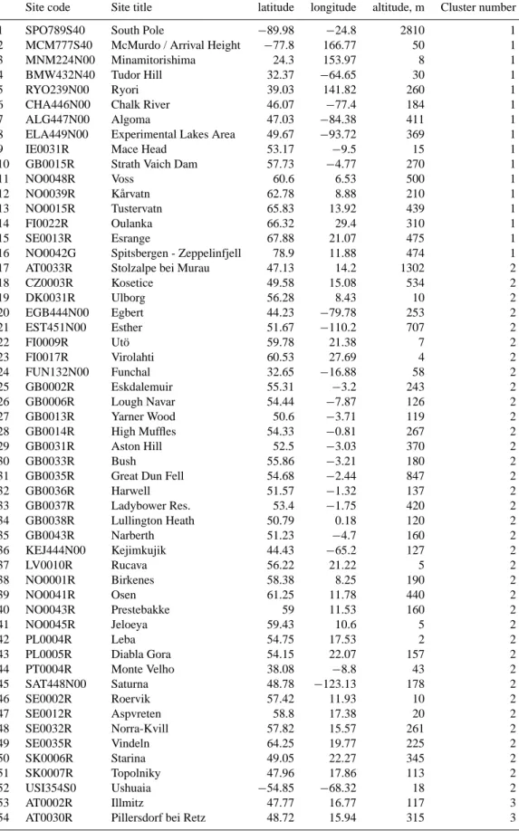
Table 1. List of the sites used for the analysis. Negative latitudes denote the Southern Hemisphere, negative longitudes denote western longitudes.
Site code Site title latitude longitude altitude, m Cluster number
1 SPO789S40 South Pole −89.98 −24.8 2810 1
2 MCM777S40 McMurdo / Arrival Height −77.8 166.77 50 1
3 MNM224N00 Minamitorishima 24.3 153.97 8 1
4 BMW432N40 Tudor Hill 32.37 −64.65 30 1
5 RYO239N00 Ryori 39.03 141.82 260 1
6 CHA446N00 Chalk River 46.07 −77.4 184 1
7 ALG447N00 Algoma 47.03 −84.38 411 1
8 ELA449N00 Experimental Lakes Area 49.67 −93.72 369 1
9 IE0031R Mace Head 53.17 −9.5 15 1
10 GB0015R Strath Vaich Dam 57.73 −4.77 270 1
11 NO0048R Voss 60.6 6.53 500 1
12 NO0039R K˚arvatn 62.78 8.88 210 1
13 NO0015R Tustervatn 65.83 13.92 439 1
14 FI0022R Oulanka 66.32 29.4 310 1
15 SE0013R Esrange 67.88 21.07 475 1
16 NO0042G Spitsbergen - Zeppelinfjell 78.9 11.88 474 1
17 AT0033R Stolzalpe bei Murau 47.13 14.2 1302 2
18 CZ0003R Kosetice 49.58 15.08 534 2 19 DK0031R Ulborg 56.28 8.43 10 2 20 EGB444N00 Egbert 44.23 −79.78 253 2 21 EST451N00 Esther 51.67 −110.2 707 2 22 FI0009R Ut¨o 59.78 21.38 7 2 23 FI0017R Virolahti 60.53 27.69 4 2 24 FUN132N00 Funchal 32.65 −16.88 58 2 25 GB0002R Eskdalemuir 55.31 −3.2 243 2 26 GB0006R Lough Navar 54.44 −7.87 126 2 27 GB0013R Yarner Wood 50.6 −3.71 119 2 28 GB0014R High Muffles 54.33 −0.81 267 2 29 GB0031R Aston Hill 52.5 −3.03 370 2 30 GB0033R Bush 55.86 −3.21 180 2
31 GB0035R Great Dun Fell 54.68 −2.44 847 2
32 GB0036R Harwell 51.57 −1.32 137 2 33 GB0037R Ladybower Res. 53.4 −1.75 420 2 34 GB0038R Lullington Heath 50.79 0.18 120 2 35 GB0043R Narberth 51.23 −4.7 160 2 36 KEJ444N00 Kejimkujik 44.43 −65.2 127 2 37 LV0010R Rucava 56.22 21.22 5 2 38 NO0001R Birkenes 58.38 8.25 190 2 39 NO0041R Osen 61.25 11.78 440 2 40 NO0043R Prestebakke 59 11.53 160 2 41 NO0045R Jeloeya 59.43 10.6 5 2 42 PL0004R Leba 54.75 17.53 2 2 43 PL0005R Diabla Gora 54.15 22.07 157 2 44 PT0004R Monte Velho 38.08 −8.8 43 2 45 SAT448N00 Saturna 48.78 −123.13 178 2 46 SE0002R Roervik 57.42 11.93 10 2 47 SE0012R Aspvreten 58.8 17.38 20 2 48 SE0032R Norra-Kvill 57.82 15.57 261 2 49 SE0035R Vindeln 64.25 19.77 225 2 50 SK0006R Starina 49.05 22.27 345 2 51 SK0007R Topolniky 47.96 17.86 113 2 52 USI354S0 Ushuaia −54.85 −68.32 18 2 53 AT0002R Illmitz 47.77 16.77 117 3
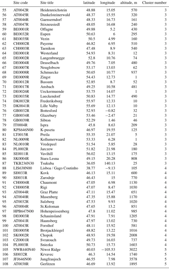
Table 1. Continued.
Site code Site title latitude longitude altitude, m Cluster number
55 AT0042R Heidenreichstein 48.88 15.05 570 3 56 AT0045R Dunkelsteinerwald 48.37 15.55 320 3 57 AT0046R Gaenserndorf 48.33 16.73 161 3 58 AT0047R Stixneusiedl 48.05 16.68 240 3 59 BE0001R Offagne 49.88 5.2 430 3 60 BE0032R Eupen 50.63 6 295 3 61 BE0035R Vezin 50.5 4.99 160 3 62 CH0002R Payerne 46.82 6.95 510 3 63 CH0003R Taenikon 47.48 8.9 540 3 64 DE0001R Westerland 54.93 8.31 12 3 65 DE0002R Langenbruegge 52.8 10.76 74 3 66 DE0004R Deuselbach 49.76 7.05 480 3 67 DE0007R Neuglobsow 53.17 13.03 62 3 68 DE0008R Schmuecke 50.65 10.77 937 3 69 DE0009R Zingst 54.43 12.73 1 3 70 DE0012R Bassum 52.85 8.7 52 3 71 DE0017R Ansbach 49.25 10.58 481 3 72 DE0026R Ueckermuende 53.75 14.07 1 3 73 DE0035R Lueckendorf 50.83 14.77 490 3 74 DK0032R Frederiksborg 55.97 12.33 10 3 75 DK0041R Lille Valby 55.69 12.13 10 3 76 GB0032R Bottesford 52.93 −0.82 32 3 77 GB0034R Glazebury 53.46 −2.47 21 3 78 GB0039R Sibton 52.29 1.46 46 3 79 IT0004R Ispra 45.8 8.63 209 3 80 KPS646N00 K-puszta 46.97 19.55 125 3 81 LT0015R Preila 55.35 21.07 5 3 82 NL0009R Kollumerwaard 53.33 6.28 1 3 83 NL0010R Vredepeel 51.54 5.85 28 3 84 PL0002R Jarczew 51.82 21.98 180 3 85 SE0011R Vavihill 56.02 13.15 175 3 86 SK0004R Stara Lesna 49.15 20.28 808 3 87 TKB236N30 Tsukuba 36.05 140.13 25 3
88 LIS638N00 Lisboa / Gago Coutinho 38.77 −9.13 105 4
89 SI0033R Kovk 46.13 15.11 600 4
90 SI0031R Zarodnje 46.43 15 770 4
91 CH0004R Chaumont 47.05 6.98 1130 4
92 CH0005R Rigi 47.07 8.47 1030 4
93 AT0044R Graz Platte 47.11 15.47 651 4
94 AT0040R Masenberg 47.35 15.88 1170 4 95 AT0032R Sulzberg 47.53 9.93 1020 4 96 AT0004R St.Koloman 47.65 13.2 851 4 97 HPB647N00 Hohenpeissenberg 47.8 11.02 985 4 98 DE0003R Schauinsland 47.91 7.91 1205 4 99 AT0041R Haunsberg 47.97 13.02 730 4 100 AT0043R Forsthof 48.11 15.92 581 4 101 DE0005R Brotjacklriegel 48.82 13.22 1016 4 102 SK0002R Chopok 48.93 19.58 2008 4 103 CZ0001R Svratouch 49.73 16.03 737 4 104 PL0003R Sniezka 50.73 15.73 1603 4 105 NWR440N40 Niwot Ridge 40.03 −105.53 3022 5 106 SI0032R Krvavec 46.3 14.54 1740 5 107 JFJ646N00 Jungfraujoch 46.55 7.98 3578 5 108 AT0038R Gerlitzen 46.69 13.92 1895 5
Table 1. Continued.
Site code Site title latitude longitude altitude, m Cluster number
109 AT0034G Sonnblick 47.05 12.96 3106 5
110 AT0037R Zillertaler Alpen 47.14 11.87 1970 5
111 NMY770S00 Neumayer −70.65 −8.25 42 6
112 SYO769S2 Syowa Station −69 39.58 29 6
113 BAR541S00 Baring Head −41.42 174.87 85 6
114 BRW471N40 Barrow 71.32 −156.6 8 6
et al. (2006). In this simulation the model dynamics has been weakly nudged in the free troposphere/lower stratosphere (up to 100 hPa) towards ECMWF operational analysis data, in order to follow the actual meteorology. For our analysis it is important to mention that most of the ozone precursor emis-sions have been prescribed for each year as monthly average fluxes of the year 2000. This could cause some discrepancy while comparing multi-annual averages of the measurements and the model output.
The model ECHAM5/MESSy1 has been compared to the other GCMs and to observations (J¨ockel et al., 2006), showing that the main processes are correctly described in the model. For instance, the stratospheric contribution in the model is 393±25 Tg(O3) y−1 and the dry deposition is 780±25 Tg(O3) y−1, which is for both processes at the lower end of the ranges presented by Stevenson et al. (2006) in the model inter-comparison experiment.
The provided model output has a time resolution of 5 h, yielding an hourly resolved diurnal cycle every 5 days. From
the ∼2.8◦×∼2.8◦ gridded model output ozone time series
at the positions of the observational sites have been sub-sampled. Due to the rather coarse model grid, some neigh-bouring sites are located in the same model grid box. Each model grid box, however, was taken into consideration only once. Thus, the number of the used model time series (72) is smaller than the actual number of sites (114) which are used for the analysis. Since the model is formulated on hybrid “terrain following” vertical layers, the lowest model level has been selected. This is feasible, since boundary layer pro-cesses, such as for instance dry deposition, are important at most of the measurement sites, with the exception of some elevated sites, at which often free tropospheric air is sam-pled. Even for these cases, it was not possible to find a non-arbitrary, strict criterion to justify sampling at higher model levels.
The model output covers the period from 1998 to 2005 and does not overlap completely with the measurement peri-ods. In addition to the ozone time series, also the simulated stratospheric ozone tracer (O(s)3 ) has been sampled (available from 2000 onward) in the same way. This tracer indicates the ozone content that originates from the stratosphere. In the analysis this information is used to estimate the contribution of the STE to the observed mixing ratios at the surface. The
STE is one of the processes controlling surface ozone vari-ability and competing to chemical production/destruction. In some cases low average mixing ratios can be accompanied by rather high stratospheric contributions being annulated for example by local destruction. Thus the obtained numbers are more indicative (qualitative) than quantitative.
3 Statistical analysis
Long-term trends of surface ozone mixing ratios can differ from site to site (e.g. in the range from +2.6±0.6%/year to −1.4±0.7%/year as reported by Virgarzan, 2004), which in-creases the uncertainty in the estimated means. To reduce possible biases and to unify the datasets, all time series were first de-trended by subtracting the incline of a linear regres-sion in time. This provides statistical uniformity of the sea-sonal variations, i.e. the averaging for each annual period should give the same mean within the range of uncertain-ties. The trend correction is between −0.8 nmol/mol/year and +1.4 nmol/mol/year and turned out to be rather different even for close locations. This issue of the trends, however, will not be discussed further in the present analysis.
For each particular location (measurement site or corre-sponding model grid box) we calculated 24 averaged sea-sonal cycles, corresponding to each hour of the day for the whole measurement/simulation period. The result is a ma-trix giving the average seasonal variation for a given time of a day and the diurnal cycle for each month simultaneously for each considered location, O3,i(h, m). Here i is the index of the measurement/simulated data location, h is the local time in hours and m is the month of the year. The number N of matrices, which were subjected to classification, is 114/72 for the measurements/model output, respectively. To obtain seasonal uniformity, the data for the Southern Hemisphere were shifted by 6 months. The model output has been shifted from universal time (UTC) to local time based on longitude information in order to synchronize it with the observations. The term cluster analysis (first used by Tryon, 1939) comprises a number of different algorithms and methods for grouping objects with similar properties into respective groups in a way that the degree of association between two objects is maximal if they belong to the same group and min-imal otherwise. Given the above, cluster analysis can be used
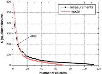
0 20 40 60 80 100 120 0 100 200 300 400 500 600 n=6 S (n ), d im e n s io n le s s number of clusters measurements model
Fig. 1. Changes of the total dispersion in the process of the agglom-eration. The optimal number of clusters for the measurements is shown in the graph (n=6) and corresponds to the point of the first strong change of S(n). For the model results the changes of S(n) are rather smooth, thus the number of clusters was selected to be the same as for the measurements.
to discover structures in data without a priori information on the data properties (Hill and Lewicki, 2006).
Basically there are two different clustering algorithms (Everitt, 1993), namely hierarchical and non-hierarchical clustering. The purpose of the hierarchical clustering is to join objects into successively larger clusters, using some
measure of similarity or distance. All the classified
ob-jects are considered at each step of the hierarchical clustering and the process is determined by the construction of an ag-glomeration (discrimination) tree. This approach is usually used when the number of clusters is unknown. A detailed overview of hierarchical classification (including agglomer-ation and discriminagglomer-ation techniques) can be found in Gor-don (1987). Hierarchical clustering is for instance often used in air transport classification (Cape et al., 2000; Colette et al., 2005).
Unlike the hierarchical clustering procedure applied here, non-hierarchical clustering (e.g. the k-means algorithm) re-quires that the number of clusters is already known and that the objects are distributed between those (Moody et al., 1991). This algorithm is widely used in cases where a priori information on the nature of the measurements is available. An example is the classification of aerosol types (Omar et al., 2005). Since we have no a priori information on the number of the particular patterns in our data, this method is not ap-plicable here.
The agglomeration hierarchical procedure begins by ini-tializing N singleton clusters (in our case one seasonal-diurnal matrix). Then the two closest clusters are merged to form a single cluster. This process is repeated until one cluster remains. Results of the agglomeration process can be different depending on the applied measure of the
dissimilar-ities (similardissimilar-ities) and distances between objects when form-ing the clusters. Normalization of the input data can also im-pact the results of classification slightly and it is usually per-formed to provide an equal weight to all the variables used for classification and to decrease the effect of the data scatter. In this paper a squared Euclidean distance is used as a measure of distance between the objects i and j :
dist2(O3,i, O3,j) = X
h,m
(O3,i(h, m) − O3,j(h, m))2, (1)
where the sum is over 24 h (h) and 12 months (m).
As an agglomeration rule the average linkage within groups is used. It takes into consideration the mean dis-tance between all possible inter- or intra-cluster pairs, unlike the average linkage method (Beaver and Palazoglu, 2006), where only the distance between the cluster averages is taken into consideration. The average distance between all pairs in the resulting cluster is minimised, min(dii), while the
aver-age distance between all the pairs in two different clusters is maximised, max(dij): d(i, j ) = ni1nj ni P s=1 nj P k=1 dist2(O3,s, O3,k), (2)
where niand nj are the number of the objects in the clusters
i and j . Since we have a rather small number of objects, the application of this agglomeration method allows us to obtain the maximum homogeneity within the clusters. In spite of the fact that the best results can be obtained with the Ward method, it is not applicable in our case as it tends to force the clusters to have similar sizes, which is not appropriate in the case of spatially inhomogeneous information.
In the agglomeration process the total distance between cluster centres and cluster members is determined at each step, representing a total dispersion S of the system
S(n) = n X i=1 nj X j =1 dist2(O3,j, O3,i), (3)
where O3,i is a centre of the cluster i, O3,j are the members of the cluster i, njis the number of the elements in the cluster
i and n is the total number of clusters. The dispersion S(n) rises monotonously and reaches its maximum when all the vectors are unified in a single cluster (n=1). The appropri-ate number of clusters is defined by the point of the extreme growth rate of S(n). The choice of the number of clusters is quite flexible if the growth rate of S(n) has no distinct ex-treme. In the case of a normal distribution of classified vec-tors, S(n) changes smoothly and the choice of the number of clusters can be rather subjective (e.g. in the case of the model output).
As stated above, we apply hierarchical agglomeration clustering to the seasonal-diurnal matrices of the measure-ments and of the model output. Figure 1 shows S(n) for both cases (measurements and model output) simultaneously. For
(a) 0 3 6 9 12 15 18 21 1 2 3 4 5 6 7 8 9 10 11 12 cluster 1 12 15 18 21 24 27 30 33 36 39 42 45 48 51 54 57 60 local time month (b) 0 3 6 9 12 15 18 21 1 2 3 4 5 6 7 8 9 10 11 12 cluster 2 12 15 18 21 24 27 30 33 36 39 42 45 48 51 54 57 60 local time month (c) 0 3 6 9 12 15 18 21 1 2 3 4 5 6 7 8 9 10 11 12 cluster 3 12 15 18 21 24 27 30 33 36 39 42 45 48 51 54 57 60 local time month (d) 0 3 6 9 12 15 18 21 1 2 3 4 5 6 7 8 9 10 11 12 cluster 4 12 15 18 21 24 27 30 33 36 39 42 45 48 51 54 57 60 local time month (e) 0 3 6 9 12 15 18 21 1 2 3 4 5 6 7 8 9 10 11 12 cluster 5 12 15 18 21 24 27 30 33 36 39 42 45 48 51 54 57 60 local time month (f) 0 3 6 9 12 15 18 21 1 2 3 4 5 6 7 8 9 10 11 12 cluster 6 12 15 18 21 24 27 30 33 36 39 42 45 48 51 54 57 60 local time month
Fig. 2. Seasonal – diurnal cycles for the 6 clusters representing 114 observed time series as described in the text. The colour scale shows the mixing ratio in nmol/mol. The following clusters are identified: (a) – clean background; (b) – rural; (c) – semipolluted nonelevated; (d) -semi-polluted semi-elevated; (e) – elevated and (f) – polar/remote.
observational data agglomeration in 6 clusters corresponds to the strong gradient of the total dispersion. At the same time the relative change of S(n) in the agglomeration of the model
data is nearly stationary. Thus, the number of the model clusters (MC) was selected to be 6, i.e. the same as for the measurements. The cluster membership was defined at the
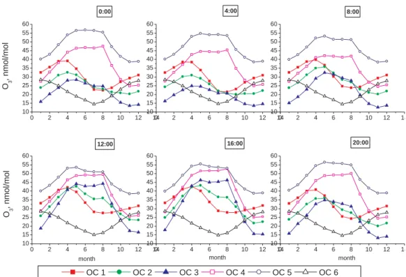
0 2 4 6 8 10 12 14 10 15 20 25 30 35 40 45 50 55 60 O3 , nmol/mol month month month O3 , nmol/mol OC 1 OC 2 OC 3 OC 4 OC 5 OC 6 0 2 4 6 8 10 12 14 10 15 20 25 30 35 40 45 50 55 60 4:00 0:00 0 2 4 6 8 10 12 14 10 15 20 25 30 35 40 45 50 55 60 16:00 12:00 8:00 0 2 4 6 8 10 12 14 10 15 20 25 30 35 40 45 50 55 60 0 2 4 6 8 10 12 14 10 15 20 25 30 35 40 45 50 55 60 20:00 0 2 4 6 8 10 12 14 10 15 20 25 30 35 40 45 50 55 60
Fig. 3. Seasonal cycle of the surface ozone mixing ratio in different measurement clusters for selected hours of the day (the data obtained as a subset of the full picture presented in Fig. 2). The mixing ratio scale is the same in all graphs to show the differences between the clusters and to reflect their diurnal changes.
corresponding step of the agglomeration procedure. Average mixing ratios (cluster centres) and their standard deviation were calculated as an average of the seasonal-diurnal cycles included in each cluster (average of the cluster members). The procedure was applied to the measurements and to the simulated data independently.
4 Results
4.1 Classes of the observed surface ozone seasonal-diurnal
cycles
The 6 typical classes (centres of the corresponding clusters) identified by the cluster analysis of the average seasonal-diurnal matrices of 114 sites are visualized in Fig. 2. The statistics of the obtained clusters for the observations and the model output are summarised in Table 2. It should be kept in mind that all estimates given in the text have a range in the order of one standard deviation listed in Table 2.
Cluster 1 (Fig. 2a) referred to as OC1 (Observational Cluster 1) is characterized by a pronounced spring maxi-mum (March–April). The values range from 21 nmol/mol to 43 nmol/mol. The months of the seasonal maximum are nearly the same for any time of the day (Fig. 3). The max-imum amplitude (difference between daily maxmax-imum and
daily minimum) of the diurnal cycle is observed in July– August (up to 7.0 nmol/mol) and is rather small. It may be explained by a combination of local chemistry (provid-ing weak daily production) and boundary layer dynamics (colder nights with stronger inversions and hence enhanced deposition at the surface). It can be seen (Fig. 2a) that in OC1 the night/early morning mixing ratios in August are the lowest throughout the year. In winter the amplitude of the diurnal variations is less than 1 nmol/mol and the absolute mixing ratios are around 30 nmol/mol. The maximum am-plitude of the seasonal variations is observed close to the time of the diurnal minimum (17 nmol/mol). It should be mentioned that the variations of the seasonal amplitude for different hours are less than 20% of its maximal magnitude. Such a regime of surface ozone variations is often reported for background/rural sites, not only in the extra tropics (e.g. Scheel et al., 1997; EMEP Assessment, 2004; Oltmans et al., 2006; Sunwoo et al., 1994), but also at some tropical loca-tions (Ahammed et al., 2006). A comparison of the prop-erties of OC1 with literature data indicates that sites in this cluster are unpolluted/remote and can be considered as repre-sentative for background conditions. Indeed, the geographic locations of the sites of this cluster (Fig. 4, Table 1) confirm this result.
Table 2. Statistical information of the observational and model clusters. One σ shows a standard deviation range in the estimate of the clusters centres (Figs. 2, 5, 7) as an average of N cluster members. Each range is representative for 288 values.
OC No. of One σ of Identified Mostly No. One σ of nmol/mol Comment One σ of sites OC centres: type (OC) over- of the MC centres: on MC MC-stratospheric
range, lapping grid range, centres:
(average), MC boxes (average), range,
nmol/mol (average), nmol/mol #1 16 2.5–7.9 clean #1 18 2.1–8.6 0.4–2.1 (4.6) back- (4.6) (1.2) ground #2 36 2.6–8.0 rural #2 30 3.5–12.1 0.4–2.1 (2.5) (5.6) (1.2) #3 35 2.4–8.3 semi- #3 15 1.0–9.3 0.2–1.6 (4.7) polluted (3.8) (0.7) non-elevated #4 17 1.8–5.2 semi-(3.4) polluted semi-elevated #5 6 1.0–6.2 elevated (2.6) #6 4 2.3–5.7 polar- #6 6 0.4–5.8 southern- 0.2–1.8 (4.1) remote (2.4) hemispheric (0.8) included in OC #5 #4 1 0 Niwot 0 Ridge
included in OC #1 and #2 #5 2 0–6.6 island 0.0–2.1
(1.9) locations (0.6)
A more complex shape of the cluster averaged seasonal-diurnal variations is observed in OC2 (Fig. 2b). Average mixing ratios in OC2 are similar to those in OC1 (19– 44 nmol/mol), while the shape of the seasonal cycle is dif-ferent. At night it is characterized by a pronounced spring maximum in April, which is shifted to May for daytime hours (Fig. 2). A secondary seasonal maximum is formed in Au-gust during the day (Fig. 3). The spring maximum of OC2 is lower than that of the background OC1 at night (up to 8 nmol/mol) and nearly equals it during daytime. At the same time the ozone mixing ratios in OC2 in winter are always (on average 9 nmol/mol) lower than that of OC1. This probably points to a higher activity of the chemical processes in OC2 in comparison with OC1, both destruction and production. Assuming that OC2 is more polluted than OC1, the lower seasonal maximum at night may be explained by ozone de-struction through reaction with NOx. This is supported by the highest differences between these clusters which are ob-served during the winter months. Higher values are obob-served in OC2 during daytime hours due to more efficient ozone production. Seasonal variations similar to those in OC2 have been reported for non-elevated rural sites, either clean or semi-polluted. The maximum amplitude of the diurnal cy-cle of OC2 is observed in August (up to 16 nmol/mol) which
is nearly 2 times larger than in background cluster OC1. In winter it does not exceed 5 nmol/mol. The maximum am-plitude of the seasonal cycle is observed at 16 h local time (22 nmol/mol). Depending on the time of the day, the ampli-tude of the seasonal cycle varies from 10 nmol/mol for early morning hours up to its maximum. These characteristics of the OC2 seasonal-diurnal variations in comparison with lit-erature information (TOR-2 Final Report, 2003; Fiore et al., 2003; Felipe-Soteloa et al., 2006; Monks, 2000) suggest that this cluster is characteristic of weakly polluted non-elevated sites (mainly rural). As can be seen in Fig. 4, the sites of OC2 are situated in Northern Europe and the mid-latitudes of the USA, mainly in the regions close to seas and on is-lands (Fig. 4). Also one of the southern hemispheric sites appears in this cluster (Ushuaia) due to the fact that average levels at this site are comparable with those in OC2, while the individual shape of the seasonal cycle is different and is characterised by a wide winter-spring maximum. This can be considered as an artefact of our approach, as it tends to merge seasonal-diurnal matrices in one cluster by trying to minimize the difference inside the cluster, and hence unify-ing members with minimum mixunify-ing ratio differences.
In comparison to the background cluster OC1, in cluster 3 (OC3), changes of the shape of the seasonal cycle are more
(a) -180 -150 -120 -90 -60 -30 0 30 60 90 120 150 180 -90 -60 -30 0 30 60 90 MEASUREMENTS cluster 1 cluster 2 cluster 3 cluster 4 cluster 5 cluster 6 Lat itu de (N ) Longitude (E) (b) -180 -150 -120 -90 -60 -30 0 30 60 90 120 150 180 -90 -60 -30 0 30 60 90 MODEL cluster 1 cluster 2 cluster 3 cluster 4 cluster 5 cluster 6 Lat itu de ( N ) Longitude (E) (c) -20 -10 0 10 20 30 30 40 50 60 70 80 MEASUREMENTS cluster 1 cluster 2 cluster 3 cluster 4 cluster 5 cluster 6 La ti tude ( N ) Longitude (E) (d) -20 -10 0 10 20 30 30 40 50 60 70 80 MODEL cluster 1 cluster 2 cluster 3 cluster 4 cluster 5 cluster 6 L a titu d e (N ) Longitude (E)
Fig. 4. Spatial distribution of the measurement sites of different clusters (a, c). The clusters obtained for the ECHAM5/MESSy1 output are also presented on the maps (b, d). For the model, the points are placed to the centre of the grid-box covering the measurement sites. In the lower panel (c–d) Europe is shown in more detail.
pronounced. Average mixing ratios in OC3 range between 12 and 47 nmol/mol with minimal values of 9 nmol/mol and of 7 nmol/mol lower than in OC1 and OC2, respectively. In contrast, the maximum mixing ratios are only 3–4 nmol/mol higher than in OC1 and OC2. OC3 is characterized by a wide spring-summer seasonal maximum (Fig. 3c). At night a spring “shoulder” of the seasonal maximum is more pro-nounced, while during daytime the spring and summer max-ima are comparable. It should be noted that during winter the ozone mixing ratios in OC3 are substantially lower than those in OC1 and OC2 at any time of the day (up to 17 nmol/mol and 8 nmol/mol, respectively), while the summer nighttime mixing ratios in OC3 are comparable to the corresponding mixing ratios in OC1 and OC2. The summer daytime mix-ing ratios in OC3 are higher than those in OC1 and OC2 (up to 19 nmol/mol and 10 nmol/mol, respectively). The spring maximum in OC3 is observed in April–May. Diurnal
max-ima and minmax-ima are observed at the same time as in OC2 at any season. The amplitude of the seasonal cycle varies from 11 nmol/mol at 5 a.m. local time to 31 nmol/mol around 3 p.m., which exceeds nearly 1.5 times the corresponding amplitude of the seasonal cycle in OC2. The amplitude of the diurnal cycle varies from 3 nmol/mol in December to 27 nmol/mol in August. Substantial variations (both seasonal and diurnal) of the surface ozone mixing ratios in OC3, the decrease during winter to values lower than the background and a substantial increase in summer, especially during day-time, point to high activity of photo-chemical processes in this cluster: strong ozone destruction by reaction with NO in winter and efficient ozone production in summer. The sub-stantially higher deviations of the ozone mixing ratios in OC3 from OC1 in comparison with similar differences between OC1 and OC2 indicate that the surface ozone variations ob-served in OC3 may be representative for more polluted sites
in comparison to OC1 and OC2 (e.g. Varotsos et al., 2001). For some sites included in OC3 (e.g. IT0004R, KPS646N00 and some others) the value of the summer maximum can ex-ceed the spring maximum, especially for daytime hours, in-dicating strong photochemical ozone production. The loca-tions of the sites of OC3 on the map (Fig. 4) show that they are likely affected by a variety of pollution sources.
OC4 (Fig. 2d) has a structure of the seasonal-diurnal cycle similar to that of OC3. Notwithstanding, the ozone levels in OC4 are higher than in OC2 or OC3 for all seasons and all times of the day (Fig. 3), i.e. in the range of 24–53 nmol/mol. This holds in winter and at night (at least 3 nmol/mol excess over OC2 and at least 11 nmol/mol excess over OC3). It is unlikely that the sites of this cluster are less polluted as far as OC2 represents rural conditions. The presence of pollution is confirmed by the fact that the winter mixing ratios in OC4 are lower than that of OC1. During the period from November till February mixing ratios at any time of the day are from 2 nmol/mol to 6 nmol/mol lower in OC4 than in OC1. In contract to OC3, in OC4 the seasonal maximum at night is not very sharp and occurs during spring and summer. Dur-ing the day the summer maximum is more pronounced and usually exceeds the spring maximum (Fig. 3). In comparison with the background OC1 spring maximum, the maximum in OC4 is two months delayed, which again indicates a higher pollution level for OC4. A similar effect was reported by Scheel et al. (2003), who showed that at Zugspitze for the more polluted years the seasonal maximum is shifted to later months. The amplitude of the diurnal cycle in OC4 varies from 1 nmol/mol in December up to 11.0 nmol/mol in Au-gust, which is 5 nmol/mol lower than in OC2 and by more than a factor of 2 less than in OC3. This means that either daily ozone production plays a less important role in OC4 in comparison with OC2 and OC3, or that the diurnal varia-tions in OC4 are less sensitive to diurnal changes of the verti-cal mixing and loverti-cal photochemistry. The comparison of the altitude ranges of sites included in OC3 and OC4, respec-tively, shows that the first group (1 m–937 m a.s.l., average 207 m a.s.l.) is less elevated than the second group (105– 2008 m, average of 952 m a.s.l.). The amplitude of the sea-sonal variations in OC4 varies from 17 nmol/mol at 7 a.m. to 28 nmol/mol at 4 p.m. Summarising the features of OC4 discussed above and comparison with the seasonal cycles in various publications (Oltmans at al., 2006, Fiore et al., 2003; Scheel et al., 2003) lead us to the conclusion that OC4 repre-sents the semi-polluted semi-elevated sites. This is confirmed by Fig. 4.
The average seasonal-diurnal cycle in the observational cluster 5 (OC5, Fig. 1e) is characterized by a broad spring-summer maximum with higher nighttime values. The aver-age mixing ratios in OC5 are in the range of 38–57 nmol/mol and they are the highest among all clusters. At night the max-ima of the seasonal variations are not distinguishable (Fig. 3), while during the day a double peak structure is present. The difference between seasonal maxima is very weak. Mixing
ratios observed in OC5 exceed those in all other clusters dur-ing all seasons and all times of the day, especially in win-ter. The excess of OC5 over the background OC1 in winter is at least 6 nmol/mol. The amplitude of the diurnal cycle varies from 0.3 nmol/mol in December to 6.0 nmol/mol in June–July, which is the period of highest insolation. These values are substantially lower than in the other clusters, ex-cept for OC6, where the diurnal cycle is absent. Since the maximum occurs at night, the diurnal cycle can be driven by boundary layer dynamics, while photochemical production only plays a minor role. The amplitude of the seasonal cycle varies from 14 nmol/mol at 9 a.m. up to 18 nmol/mol between 10 p.m. and 12 p.m. The rather stable high mixing ratios and the seasonal variations are nearly insensitive to the time of the day (with a slight growth at night) and most likely corre-spond to the surface ozone regime observed at mountain sites (Oltmans at al., 2006; Fiore et al., 2003; Scheel et al., 2003; Schuepbach et al., 2001; Tarasova et al., 2003). Presenting the members of OC5 on the map indeed shows elevated loca-tions (Fig. 4). The summary in Table 2 shows that there are 6 locations included in OC5, all with elevations of more than 1700 m a.s.l. (Table 1).
The structure of the observational cluster 6 (OC6) demon-strates how sites with different mechanisms influencing the seasonal and diurnal variations can appear in the same cluster due to comparable mixing ratio levels and due to similarities of the seasonal variations . OC6 includes 4 sites, situated in the coastal zone of the Arctic (Barrow) and Antarctica (Neu-mayer and Syowa Station) and a site in New Zealand (Baring Head) (Fig. 4). The mixing ratios in OC6 range between 14 and 29 nmol/mol. Three other sites of the Southern Hemi-sphere are considered in the analysis, namely South Pole and McMurdo, which are in OC1, and Ushuaia in cluster OC2. These sites have higher mixing ratios and they are assigned to the other clusters with more appropriate levels. In fact the shape of the seasonal-diurnal variations is quite similar for all southern hemispheric locations. OC6 is characterized by a pronounced winter (local June–July) seasonal maximum. Note that southern hemispheric data were 6 months shifted prior to the analysis. The winter seasonal maximum is ob-served at all times of the day and in absence of diurnal varia-tions (Fig. 2). Such a shape of the seasonal cycle is reported for the majority of the mid- and high-latitude locations of the Southern Hemisphere, in particular for Cape Point, Cape Grim, South Pole and others (Oltmans et al., 2006; 2007; Scheel et al., 1990; Gros et al., 1998). The diurnal variations in this cluster are very weak and do not exceed 1 nmol/mol. This absence of diurnal variations indicates that the surface ozone variability is controlled by the processes with time-scales longer than a day. The amplitude of the seasonal cycle in OC6 reaches 14 nmol/mol and does not depend on the time of the day. The high stability of ozone at the sites in OC6 probably shows that atmospheric transport can be more important for these sites than local fast photochemistry. The surface ozone variation represented by OC6 occurs at those
locations where photochemical activity is weak because of low precursor levels and/or because of the low levels of sun-light and/or because chemical destruction does not play a role in winter (such as in polar regions or on remote islands). The map (Fig. 4) shows that OC6 comprises the sites situated in the polar (or close to polar) coastal zones of Antarctica, New Zealand and Alaska. It is likely that photochemical processes are more important at these locations for the formation of the seasonal minimum through ozone destruction in spring-summer (reactions with bromine compounds), while photo-chemical production is very unlikely. The seasonal max-imum at these locations is more plausibly connected with transport processes, both vertical motions (STE) and hori-zontal advection.
4.2 Classes of model simulated surface ozone
seasonal-diurnal cycles
To compare the features of the clusters obtained for the mea-surement sites with the results from the global model simu-lation, we applied the same technique to the sampled model output at the grid boxes covering the measurement locations. For the model results we applied the hierarchical clustering procedure and stopped the agglomeration algorithm at 6 clus-ters to compare the obtained cluster centres with those ob-tained for the measurements. It should be noted (see Table 2 for details) that the majority of the grid boxes are covered by 3 large clusters, while two clusters contain only one or two grid boxes.
Similar to the measurements, the mean seasonal-diurnal cycles of the model clusters (MC) are presented in Fig. 6. As additional information used for the interpretation of the stud-ied variations, the mean stratospheric contribution calculated for each model cluster is presented (Fig. 7). This parameter is used to indicate the role of stratosphere-to-troposphere trans-port and its changes throughout the year for each particular model cluster. Figure 7a shows the stratospheric contribu-tion in absolute values, while Fig. 7b shows it in relative val-ues to the average mixing ratio observed in the model clus-ters. It should be noted that these values are used only as a qualitative indication rather than a quantitative estimate. An excess of the relative contribution over 100% shows that in situ chemical destruction exceeds local production + strato-spheric contribution. The maximum of the stratostrato-spheric con-tribution in absolute values is observed in February–March
(Fig. 7a) depending on the cluster. Differences between
February and March are usually within the range of uncer-tainty of the clusters’ average (see last column of Table 2). Some errors can arise in these estimates due to the differ-ent time coverage of the considered data sets (1990–2004 for the measurements, 1998–2005 for the model output mixing ratios and 2000–2005 for the stratospheric contribution esti-mate).
The comparison of the main properties of the observa-tional clusters and the ECHAM5/MESSy1 model clusters, respectively (Figs. 1 and 4), shows that the model reproduces the main classes of the observed variations reasonably well. The following classes are represented by the model: a cluster with a winter-early spring seasonal maximum and a less pro-nounced diurnal cycle (analogous to OC6); a cluster with a spring maximum and a well established diurnal cycle (anal-ogous to OC1); a cluster with spring-summer maxima and a developed diurnal cycle (comparable to OC2 and OC3); a cluster with elevated mixing ratios (throughout the year), a pronounced seasonal spring maximum and a very weak diur-nal cycle with an amplitude independent of the season (sim-ilar to OC5); and a cluster with a developed seasonal max-imum in summer and a strong diurnal cycle. The last two regimes are likely to be similar to OC3 and OC4.
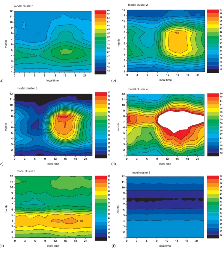
The model cluster 1 (MC1) by the shape of its seasonal-diurnal matrix is comparable to OC1. It contains 18 grid boxes. Mixing ratios range in MC1 from 20 nmol/mol to 40 nmol/mol, which is close to the range of the mixing ratios in OC1 (21–43 nmol/mol) and OC2 (19–44 nmol/mol). The average seasonal-diurnal cycle in MC1 presented in Fig. 5a is characterised by the pronounced spring maximum in April– May. The seasonal maximum is observed in April during night and early morning hours, while for daytime the maxi-mum is shifted to May (Fig. 6). This is one month later than in the background cluster OC1 and coincides with the timing of the seasonal maximum in the rural cluster OC2 (Fig. 8a). The deviation of the daily average mixing ratios in MC1 from those in OC2 (Fig. 9) shows that in winter the simu-lated mixing ratios are slightly higher (less than 2 nmol/mol) than those in OC2, while in summer (June–August) they are up to 4 nmol/mol lower than in OC2. The summer mixing ratios in MC1 are close to those of OC1 and exceed them by less than 2 nmol/mol. In general, the shape of the seasonal-diurnal matrix of MC1 is closer to that of OC2 than to that of OC1. The amplitude of the seasonal cycle in MC1 varies from 11 nmol/mol at night to its maximum of 17 nmol/mol at 5 p.m. This range is similar to that of OC1. The excess of the diurnal maximum in summer of about 5 nmol/mol and the winter deficit of around 10 nmol/mol in MC1 in com-parison with OC1 indicate the overestimated contribution of photochemical production/destruction for the grid boxes in MC1. The amplitude of the diurnal cycle in MC1 varies from 1 nmol/mol in December–January to its maximum in July– August (up to 11 nmol/mol), which is a bit higher than that in OC1. The difference of the mixing ratios in MC1 and OC1 in winter is higher than the dispersion of the cluster centres and is likely caused by the above mentioned overestimated destruction. The stratospheric contribution in MC1 does not exceed 60% in winter and 10% in summer. The map showing the locations of the MC1 grid boxes indeed indicates unpol-luted locations (in Fig. 4 MC1 is mostly overlapping with OC1).
(a) 0 3 6 9 12 15 18 21 1 2 3 4 5 6 7 8 9 10 11 12 model cluster 1 12 15 18 21 24 27 30 33 36 39 42 45 48 51 54 57 60 local time month (b) 0 3 6 9 12 15 18 21 1 2 3 4 5 6 7 8 9 10 11 12 model cluster 2 12 15 18 21 24 27 30 33 36 39 42 45 48 51 54 57 60 local time month (c) 0 3 6 9 12 15 18 21 1 2 3 4 5 6 7 8 9 10 11 12 model cluster 3 12 15 18 21 24 27 30 33 36 39 42 45 48 51 54 57 60 local time month (d) 0 3 6 9 12 15 18 21 1 2 3 4 5 6 7 8 9 10 11 12 model cluster 4 12 15 18 21 24 27 30 33 36 39 42 45 48 51 54 57 60 local time month (e) 0 3 6 9 12 15 18 21 1 2 3 4 5 6 7 8 9 10 11 12 model cluster 5 12 15 18 21 24 27 30 33 36 39 42 45 48 51 54 57 60 local time month (f) 0 3 6 9 12 15 18 21 1 2 3 4 5 6 7 8 9 10 11 12 model cluster 6 12 15 18 21 24 27 30 33 36 39 42 45 48 51 54 57 60 local time month
Fig. 5. Seasonal-diurnal ozone cycles for the 6 clusters of the ECHAM5/MESSy1 model output sub-sampled at the measurement sites. Colours and units are as in Fig. 2.
The model cluster 2 (MC2) by its absolute values (16– 51 nmol/mol) is closer to OC3 (Fig. 5b) than to OC2. Around half of the grid boxes are contained in this cluster (30 of 72). This cluster is characterized by a broad spring-summer
max-imum. As can be seen in Fig. 6 such a shape of the seasonal cycle is present at all times of the day, while it is more likely to show a double peak structure for nighttime hours. It is in-teresting to note that during the day absolute mixing ratios
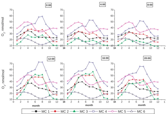
0 2 4 6 8 10 12 14 10 20 30 40 50 60 70 O3 , nmol/mol month month month O3 , nmol/mol MC 1 MC 2 MC 3 MC 4 MC 5 MC 6 0 2 4 6 8 10 12 14 10 20 30 40 50 60 70 4:00 0:00 0 2 4 6 8 10 12 14 10 20 30 40 50 60 70 16:00 12:00 8:00 0 2 4 6 8 10 12 14 10 20 30 40 50 60 70 0 2 4 6 8 10 12 14 10 20 30 40 50 60 70 20:00 0 2 4 6 8 10 12 14 10 20 30 40 50 60 70
Fig. 6. Seasonal cycle of the surface ozone mixing ratio in different model clusters for selected hours of the day (the data obtained as a subset of the full picture presented in Fig. 5, similar to Fig. 3 for the measurements).
of the both (spring and summer) maxima grow (Fig. 6). This is similar to the diurnal development of the seasonal cycle in OC3 (Fig. 3). But unlike OC3, where during daytime the summer maximum gets more pronounced, the shape of the seasonal cycle in MC2 is similar for day and night (only the absolute values are growing). This likely implies that local photo-chemical production does not play a primary role and the production is of a more regional impact (the growth is provided by the growing “background” mixing ratios). The amplitude of the seasonal cycle varies from 16 nmol/mol at 7 a.m. to 32.9 nmol/mol at 2–3 p.m. The maximum ampli-tude of the seasonal cycle in MC2 exceeds both correspond-ing values for OC2 and OC3. Comparison of MC2 and OC2 (Fig. 8b) shows that during summer not only the maximum, but also the minimum values are higher in MC2 than in OC2, e.g. in July–August the diurnal minimum is overestimated by around 5 nmol/mol. Since nighttimes values can not be explained by overestimated production, this could indicate a positive bias of the simulated values in comparison to the measurements. Further checks did not reveal any systematic shift. The stratospheric contribution reaches its maximum in MC2 in March (16.5 nmol/mol) and it does not exceed 5 nmol/mol in summer. These values contribute up to 80% of the average mixing ratio in winter and up to 15% in sum-mer. It is less plausible that the stratospheric contribution is overestimated in this cluster, causing a substantial deviation
from OC2. The map (Fig. 4b, d) shows that MC2 covers a part of Northern Europe by a wide belt along the coast, the Alps , some mid-latitude rural sites of the USA and islands (Japan). Thus the possible reason for the elevated ozone mix-ing ratios in MC2 in comparison with OC2 is that MC2 cov-ers semi-elevated and mountain locations. Since the model is formulated on terrain following vertical coordinates, it will represent to some extent elevated locations. This results in higher ozone mixing ratios in comparison to the measure-ments (where semi-elevated and mountain sites are separated into different clusters). This statement is also confirmed by a slight shift of the diurnal cycle in MC2 to later hours in comparison to OC2.
The model cluster 3 (MC3) has a mean seasonal-diurnal matrix similar to those of MC2 and OC3 (Fig. 5c) and is char-acterized by a wide spring-summer maximum. The range of the mixing ratios in MC3 is wider than those in MC1 and MC2 and amounts to 9–58 nmol/mol. As for OC3, the seasonal cycle in MC3 changes during the day. For night-time hours the spring and summer maxima are comparable. For daytime hours the spring maximum is not pronounced and the summer mixing ratios exceed the spring mixing ra-tios (April–May) by 6 nmol/mol (Fig. 6). This indicates lo-cal photochemilo-cal ozone production. The amplitude of the seasonal cycle strongly depends on the time of the day and varies from 10 nmol/mol at 6 a.m. to 47 nmol/mol at 2 p.m.,
(a) 2 4 6 8 10 12 14 16 18 20 22 24
Jan Feb Mar Apr May Jun Jul Aug Sep Oct Nov Dec
O 3 , nmol/mol MC 1 MC 2 MC 3 MC 4 MC 5 MC 6 (b) 0 10 20 30 40 50 60 70 80 90 100 110
Jan Feb Mar Apr May Jun Jul Aug Sep Oct Nov Dec
O 3, strat /O 3, ave *100, % MC 1 MC 2 MC 3 MC 4 MC 5 MC 6
Fig. 7. Stratospheric contribution to the surface ozone averaged for each model cluster in absolute values (a) and as a relative contribution to the simulated mixing ratios (b). In the figure the averaged diurnal cycles are presented for every month. Error bars are not presented for the sake of visibility of the data and instead are summarized in Table 2.
(a) 20 25 30 35 40 45
Jan Feb Mar Apr May Jun Jul Aug Sep Oct Nov Dec O3 , nmol/mol OC 1 OC 2 MC 1 (b) 15 20 25 30 35 40 45 50 55
Jan Feb Mar Apr May Jun Jul Aug Sep Oct Nov Dec O3 , nmol/mol OC 2 MC 2 (c) 5 10 15 20 25 30 35 40 45 50 55 60
Jan Feb Mar Apr May Jun Jul Aug Sep Oct Nov Dec O3 , nmol/mol OC 3 MC 3 (d) 10 15 20 25 30 35
Jan Feb Mar Apr May Jun Jul Aug Sep Oct Nov Dec O3
, nmol/mol
OC 6 MC 6
Fig. 8. Comparison of the seasonal-diurnal cycle between spatially overlapping clusters of the measurements and the model results as presented in Table 2. As in Fig. 7, the lines show average diurnal cycles for each month.
0 2 4 6 8 10 12 -8 -6 -4 -2 0 2 4 6 8 10 12 daily mean (O 3, mod - O 3, obs ), nmol/mol month MC1-OC1 MC1-OC2 MC2-OC2 MC3-OC3 MC6-OC6
Fig. 9. Seasonal cycle of daily averaged difference between mostly or partly overlapping model and observation clusters.
indicating the connection of the seasonality with local pho-tochemical activity. A strong production also causes strong diurnal variations in summer. Nevertheless, Fig. 8c demon-strates a quite good agreement between MC3 and OC3 in winter. Moreover, the daytime mean values support a com-parison of MC3 and OC3 (Fig. 9), indicating that the model overestimate in summer is less than 4 nmol/mol and the max-imum underestimation in the other seasons is 5 nmol/mol. Taking into consideration the uncertainty of the cluster cen-tres this comparison provides a good result. For both the model and measurement clusters (MC3 and OC3) the max-imum of the diurnal variations is observed in August and
reaches 43 nmol/mol and 27 nmol/mol, respectively.
Fig-ure 7b shows that the relative contribution of stratospheric ozone to the average mixing ratios exceeds 100% in winter, which means that the chemical ozone destruction exceeds the total production and the flux from the stratosphere. There-fore, the observed mixing ratios are even lower than the mix-ing ratios of the stratospheric tracer. The maximum overes-timate of MC3 over OC3 is around 10 nmol/mol in summer at the diurnal maximum, while the simulated diurnal minima are less than 8 nmol/mol lower than those of the measure-ments. Taking into consideration the limitations of the global model and the difference in the covered periods, the agree-ment between MC3 and OC3 can be considered as rather good. The map (Fig. 4) of the cluster distribution shows that MC3 contains 15 grid boxes covering the sites of Central Eu-rope and rural sites in the USA. Since MC3 is centred in Cen-tral Europe, the problem of the elevation which impacts MC2 is not so critical in this cluster.
The model cluster 4 (MC4) presents a special case (Fig. 5d). This cluster consists of only one grid box, cor-responding to Niwot Ridge , i.e. an elevated site in the USA. This cluster is characterised by the highest (among MC and OC) mixing ratios in the range of 24–73 nmol/mol. It has a
seasonal-diurnal cycle with a very strong summer maximum, which is observed at all times of the day (Fig. 6). The win-ter mixing ratios in MC4 are also relatively high, with values typical for semi-elevated and mountain locations (the low-est mixing ratios in MC4 equal those in OC4, which is rep-resentative of semi-elevated semi-polluted conditions). But unlike OC4, the diurnal and seasonal variations in this clus-ter are much stronger: the seasonal cycle amplitude ranges from 26 nmol/mol at 8 a.m. to 45 nmol/mol at 11 a.m. in MC4 compared to 17 nmol/mol at 7 a.m. to 28 nmol/mol at 4 p.m. in OC4; the diurnal cycle amplitude ranges from 8 nmol/mol in December to 22 nmol/mol in August in MC4 compared to 1 nmol/mol in December to 11 nmol/mol in August in OC4. This is an indication that MC4 shows an elevated location with very strong photochemical ozone production. One more feature of this cluster is the highest stratospheric contribution in comparison with other model clusters (Fig. 7). It is diffi-cult to judge whether this is a real excess, or whether averag-ing within the clusters smoothes out similar elevated contri-butions for other particular locations. Also, it is interesting to see that the diurnal variations of the stratospheric contri-bution in MC4 are much stronger than in the other model clusters, but it is nearly constant in relative units and does not exceed 55%.
The model cluster 5 (MC5) is represented by two grid-boxes only. The average seasonal-diurnal variations in this cluster are presented in Fig. 5e. It is characterized by rela-tively high (the highest in winter in comparison with all the other model clusters) mixing ratios with a rather broad spring maximum (April). The range of the mixing ratios in MC4 is 32–52 nmol/mol. This range is close to the range reported above for OC5 (38–57 nmol/mol), but the shape of the sea-sonal cycle is completely different. Unlike the other clusters, the seasonal minimum in OC5 is observed in July. The di-urnal cycle in MC5 is rather weak, reaching its maximum in August (3.7 nmol/mol). It is likely that in this cluster the surface ozone is controlled by the processes with time-scales longer than a day. Since a slight increase in the mixing ratio occurs in the evening and the seasonality is characterized by the spring maximum only, this regime is characteristic of un-polluted locations with weak boundary layer photochemistry and dynamics. Elevated night and winter mixing ratios in comparison with background conditions can indicate either elevated locations (but then a secondary maximum should form in summer) or remote locations with reduced dry de-position. This is likely the case of observations over water surfaces. Figure 4 shows that the two locations represent-ing MC5 are islands and hence, cluster MC5 represents the seasonal-diurnal cycle of the surface ozone over the ocean. It should be noted that the stratospheric relative contribution in MC5 never exceeds 45% (Fig. 7b) and the diurnal varia-tions are weak. This supposes that elevated mixing ratios in comparison with the other clusters are due to the lower depo-sition over the water surface instead of a stronger flux from the stratosphere or stronger photochemical production.
The model cluster MC 6 (Fig. 5a) by its properties looks
rather similar to OC6. This cluster is characterized by
the lowest (in comparison with other model or observa-tional clusters) ozone mixing ratios, in the range from 12 to 23 nmol/mol. This range is comparable to that of OC6 (14– 29 nmol/mol). The seasonal maximum in MC6 is observed in March, coinciding in time with the maximum of the strato-spheric contribution. In fact (Fig. 7a) the stratostrato-spheric con-tribution in absolute values does not change significantly be-tween January and March and is at the level of 12 nmol/mol. Similar to OC6, the diurnal cycle in MC6 is absent. Compar-ison of the seasonal-diurnal cycles for OC6 and MC6 (Fig. 8d and Fig. 9) shows that unlike the observations where the sea-sonal maximum is observed in winter (December-January), the seasonal maximum in MC6 is shifted to spring. The seasonal minimum in summer is reproduced in MC6, but 1 month later (in August) in comparison to OC6 (July). For the period from March to August the difference between the mixing ratios in MC6 and OC6 is less than 5 nmol/mol. The largest differences between MC6 and OC6 are observed in autumn and winter, but still the model underestimates the observations by less than 8 nmol/mol. The absolute strato-spheric contribution in this cluster is the lowest (12 nmol/mol at maximum), while the relative contribution is up to 55% (Fig. 7b). Analysing the geographical distribution of the grid-boxes contained in this cluster, we find southern hemi-spheric locations and the grid box containing Barrow. At the moment it is unclear why the model underestimates po-lar/remote mixing ratios and why a shift of the seasonality is observed in the model. One possibility is an underestimated flux from the stratosphere, however, we do not have the data to check this hypothesis (an analysis of the ozone sounding data is necessary). It is unlikely that background concentra-tions in the Southern Hemisphere are underestimated: a site-by-site comparison of model results and the observations (in-cluding Barrow) does not reveal any systematic differences. In total there are only 6 grid-boxes contained in MC1 cover-ing 3 locations (of 4) representative for the similar regime in the measurements. Thus, it can be concluded that the vari-ations of the surface ozone at remote locvari-ations, taking into consideration the limitations of the model setup and the un-certainty in the cluster centre detection, are captured reason-ably well by the model.
5 Conclusions
In this study the main features of the surface ozone seasonal-diurnal variations are discussed. A statistical approach was applied to classify the main types of the seasonal-diurnal cycles based on the measurement data of 114 sites and the output from an atmospheric chemistry general circulation model. Some limitations in the analysis arose from the non-uniform spatial data coverage which makes the results more representative of the Northern Hemisphere. Nevertheless the
obtained features represent the main global features of the surface ozone variations.
Our approach revealed 6 typical classes of the seasonal-diurnal cycles in the measurements. Background locations are characterized by a pronounced spring maximum which appears independent of the time of day. We conclude that it is probably not driven by local photochemical processes, but is rather of a dynamical origin. Four measurement clusters are characterized by a broad spring-summer maximum, where the summer part is more pronounced for daytime hours and plausibly due to photochemical production. A strong differ-ence is seen between rural, semi-polluted non-elevated and semi-polluted semi-elevated sites with a more stable struc-ture (less variability) and enhanced mixing ratios through-out the year for the latter. Polar/remote locations are also localized in one cluster and they are characterized by low absolute mixing ratios, a pronounced winter maximum and the absence of diurnal variations. It should be noted that both northern and southern hemispheric locations have such a regime of the surface ozone variations.
As for the measurements, the statistical approach has also been applied to model output. While making the compari-son between the observed and the simulated seacompari-sonal-diurnal cycles, it should be kept in mind that the model data have different temporal and spatial resolution, and that identical monthly emissions have been prescribed each year. Never-theless, the agreement between the model clusters and the observation clusters is rather good. We used the same num-ber of clusters for the model output as for the measurements. The regime with low mixing ratios and without a diurnal cy-cle is reproduced by the model for 5 of 6 considered grid boxes of the Southern Hemisphere and for Barrow. 3 of 4 sites included in the corresponding cluster of observations are overlapping with this model cluster. The seasonal max-imum in the model simulation is shifted to March and the minimum is shifted to August, which are respectively 2 and 1 months later than in the corresponding observational clus-ter. Background, rural and semi-polluted sites are merged for the model output in different clusters. For the cluster cover-ing background locations the seasonal maximum is observed in April–May. For the model cluster covering rural loca-tions and for the cluster covering semi-polluted localoca-tions the role of the photochemical production/destruction is likely to be overestimated, resulting in too low winter values and too high summer production. The amplitude of the diurnal cycle for the summer months in the more polluted cluster exceeds 40 nmol/mol. At the same time the excess of the rural mixing ratios can be explained by a bias resulting from the applied de-trending procedure, which normalises to the beginning of the data period, which is different for the model compared to the observations. Furthermore, the inclusion of elevated locations in this cluster contributes to this bias. Taking into consideration the differences in the data sampling procedure (initial temporal resolution, the coarse spatial model resolu-tion and the difference in the covered period), the obtained