HAL Id: hal-00295757
https://hal.archives-ouvertes.fr/hal-00295757
Submitted on 18 Oct 2005
HAL is a multi-disciplinary open access
archive for the deposit and dissemination of
sci-entific research documents, whether they are
pub-lished or not. The documents may come from
teaching and research institutions in France or
abroad, or from public or private research centers.
L’archive ouverte pluridisciplinaire HAL, est
destinée au dépôt et à la diffusion de documents
scientifiques de niveau recherche, publiés ou non,
émanant des établissements d’enseignement et de
recherche français ou étrangers, des laboratoires
publics ou privés.
surfaces in the identification of cloud-free observations
using SCIAMACHY PMDs
J. M. Krijger, I. Aben, H. Schrijver
To cite this version:
J. M. Krijger, I. Aben, H. Schrijver. Distinction between clouds and ice/snow covered surfaces in
the identification of cloud-free observations using SCIAMACHY PMDs. Atmospheric Chemistry and
Physics, European Geosciences Union, 2005, 5 (10), pp.2729-2738. �hal-00295757�
Atmos. Chem. Phys., 5, 2729–2738, 2005 www.atmos-chem-phys.org/acp/5/2729/ SRef-ID: 1680-7324/acp/2005-5-2729 European Geosciences Union
Atmospheric
Chemistry
and Physics
Distinction between clouds and ice/snow covered surfaces in the
identification of cloud-free observations using SCIAMACHY PMDs
J. M. Krijger, I. Aben, and H. Schrijver
SRON, National Institute for Space Research, Sorbonnelaan 2, 3584 CA Utrecht, The Netherlands Received: 20 December 2004 – Published in Atmos. Chem. Phys. Discuss.: 14 February 2005 Revised: 20 June 2005 – Accepted: 23 September 2005 – Published: 18 October 2005
Abstract. SCIAMACHY on ENVISAT allows measurement
of different trace gases including those most abundant in the troposphere (e.g. CO2, NO2, CH4, BrO, SO2). However,
clouds in the observed scenes can severely hinder the ob-servation of tropospheric gases. Several cloud detection al-gorithms have been developed for GOME on ERS-2 which can be applied to SCIAMACHY. The GOME cloud algo-rithms, however, suffer from the inadequacy of not being able to distinguish between clouds and ice/snow covered sur-faces because GOME only covers the UV, VIS and part of the NIR wavelength range (240–790 nm). As a result these areas are always flagged as clouded, and therefore often not used. Here a method is presented which uses the SCIAMACHY measurements in the wavelength range between 450 nm and 1.6 µm to make a distinction between clouds and ice/snow covered surfaces. The algorithm is developed using collo-cated MODIS observations. The algorithm presented here is specifically developed to identify cloud-free SCIAMACHY observations. The SCIAMACHY Polarisation Measurement Devices (PMDs) are used for this purpose because they pro-vide higher spatial resolution compared to the main spec-trometer measurements.
1 Introduction
Satellite-based passive remote sensing is commonly used to derive global information about the composition of the Earth’s atmosphere. Information about the total column or even vertical profiles of different gases in the Earth atmo-sphere can be obtained by measuring the radiance (intensity) spectrum of sunlight reflected by the Earth’s atmosphere, since these spectra contain absorption bands of gases present in the atmosphere, such as ozone. In the ultra-violet (UV), Correspondence to: J. M. Krijger
visible (VIS) and near infra-red (NIR) wavelength range the presence of clouds can strongly affect the observation of constituents in the troposphere, because clouds effectively screen the lower part of the atmosphere. When clouds are not properly accounted for, and especially when a significant part of the airmass of interest is below the cloud, (large) er-rors are introduced. Therefore, cloud detection algorithms are of crucial importance in satellite remote sensing.
The SCanning Imaging Absorption SpectroMeter for At-mospheric CHartographY (SCIAMACHY) is a joint Ger-man/Dutch/Belgian instrument on board the ESA ENVISAT satellite, which was launched on March 1st 2002 and is ex-pected to operate for at least five years. SCIAMACHY is a grating spectrometer measuring the radiance of reflected and back-scattered sunlight between 240–2380 nm at 0.2–1.5 nm spectral resolution. In order to account for the instrument po-larisation sensitivity, SCIAMACHY measures the polarisa-tion of reflected sunlight using seven broadband detectors, re-ferred to as the Polarisation Measurement Devices (PMDs).
The predecessor of SCIAMACHY, the Global Ozone Monitoring Experiment (GOME), was launched on 21 April 1995 on-board ESA’s second European Remote Sensing satellite (ERS-2). GOME is a de-scoped version of SCIA-MACHY and only covers the ultraviolet, visible and near-infrared wavelength range from 240 to 790 nm with 0.2– 0.4 nm spectral resolution (Burrows et al., 1999). GOME is also equipped with three broadband PMDs, measuring po-larised light across its full wavelength range.
Several cloud detection algorithms were developed for use in GOME, like ICFA (Kuze and Chance, 1994), OCRA (Loyola, 1998), CRAG (von Bargen et al., 2000), CRUSA (Wenig, 2001), FRESCO (Koelemeijer et al., 2001), GOME-CAT (Kurosu et al., 1998), HICRU (Grzegorski et al., 2004) and SACURA (Rozanov and Kokhanovsky, 2004). These methods either use the high spectral resolution measure-ments from the main spectrometer, or the broadband PMD measurements, or a combination of both. Some of these
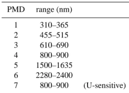
Table 1. Wavelength ranges SCIAMACHY Polarisation
Measure-ment Devices, containing 80% of the signal.
PMD range (nm) 1 310–365 2 455–515 3 610–690 4 800–900 5 1500–1635 6 2280–2400 7 800–900 (U-sensitive)
algorithms have been modified for use with SCIAMACHY measurements, but since GOME does not measure in the infra-red region none of these methods uses information in the infra-red wavelengths beyond 800 nm as measured by SCIAMACHY. Because both clouds and ice/snow cov-ered surfaces are highly reflective and white in the GOME wavelength range, none of these algorithms distinguish be-tween clouds or ice/snow covered surfaces in the observa-tion. While in principle cloud detection methods using the O2A band, like FRESCO and SACURA, can detect the
pres-sure of the clouds or the surface and thus discriminate white clouds from a white surface, this is not part of the current ver-sions of these algorithms. Without the ability to distinguish between cloudy and ice/snow covered surfaces, all observa-tions over ice/snow covered surfaces are flagged as cloudy and therefore often not used. A method to distinguish be-tween clouds and ice/snow covered surfaces is thus of crucial importance to be able to identify cloud-free observations.
Here the SCIAMACHY PMD Identification of Clouds and Ice/snow method (SPICI) is presented which is a variation on previous cloud-detection algorithms. It uses, a.o. the SCIAMACHY PMD measurements in the wavelength range around 1.6 µm where the reflectivity of ice/snow covered sur-faces is significantly reduced while the reflectivity of clouds is still high. Using this clear spectral difference in reflectiv-ities a distinction between clouds and ice/snow covered sur-faces in the SCIAMACHY observations can be made. The algorithm consists of two steps. In the first step the algo-rithm only uses PMD 2, 3 and 4 to determine the presence of a white surface in the visible wavelength range. Because at these wavelengths one can not separate clouds from ice/snow covered surfaces, a second step is needed to finally detect cloud-free observations also over ice/snow covered surfaces. Because the SCIAMACHY PMDs are not radiometrically calibrated, the SPICI algorithm is developed using collocated high spatial resolution observations from MODIS on Eos-Terra.
The structure of this paper is as follows. In Sect. 2 we describe the Polarisation Measurement Devices on-board SCIAMACHY and present some illustrations of their use in
colour images of the Earth which illustrates the basic con-cept for the cloud and ice/snow algorithm SPICI presented in Sects. 3 and 4. Section 3 starts with the definition of the cloud algorithm which represents the first step in the SPICI algorithm. Section 4 deals with the actual distinction be-tween clouds and ice/snow covered surfaces. Validation of the SPICI algorithm is presented in Sect. 5. We finish with a summary in Sect. 6.
2 SCIAMACHY Polarisation Measurements Devices
2.1 SCIAMACHY
SCIAMACHY’s primary mission objective is to perform global measurements of trace gases in the troposphere and stratosphere (Bovensmann et al., 1999). The instrument provides column and/or vertical profile information on O3,
H2CO, SO2, BrO, OClO, NO2, H2O, CO, CO2, CH4, N2O,
O2, (O2)2, and on clouds and aerosols as well.
SCIA-MACHY thereto measures the radiance of reflected and back-scattered sunlight in 8 channels, covering the 240– 1750 nm wavelength (channels 1–6) and two IR bands 1940– 2040 nm and 2265–2380 nm (channels 7 and 8, respectively) at 0.2–1.5 nm spectral resolution. SCIAMACHY alternates between nadir and limb viewing modes for most part of the orbit. The swath of the instrument in nadir mode is 960 km, and the individual main channel measurements have a foot-print on Earth ranging from 60 km×30 km to 240 km×30 km (across × along track), thereby providing global coverage in a period of six days (Bovensmann et al., 1999).
2.2 SCIAMACHY PMD measurements
SCIAMACHY is a highly polarisation-sensitive instrument due to the instrument’s gratings and mirrors. Neglect of such an instrument’s polarisation sensitivity can lead to errors in the radiances of several tens of percents at wavelengths where the instrument polarisation sensitivity is highest. In or-der to correct for this polarisation sensitivity, SCIAMACHY measures the polarisation of reflected sunlight using seven broadband detectors, referred to as Polarisation Measure-ment Devices (PMDs, see Table 1), which roughly cover the spectral range of the main spectrometer. Because the PMDs are mainly sensitive to parallel (to the instrument slit) po-larised light, while the main channel spectrometer is sensitive to both polarisation components, information on the polari-sation of the incoming light is obtained by combining the two measurements (Slijkhuis, 2000). The PMDs are read out at 40 Hz, but are down-sampled to 32 Hz for processing. This still gives a much better spatial resolution (∼7 km×30 km) than the main spectral channels where the fastest read-out occurs at 8 Hz, and more commonly at 1 Hz. This high PMD spatial resolution allows us to study clouds and ice/snow in more spatial detail which is the reason why we use the PMDs
J. M. Krijger et al.: SCIAMACHY PMDs Identification of Clouds and Ice/snow 2731
Fig. 1. Earth surface as seen by SCIAMACHY PMD 2, 3, and
4. The Earth surface was gridded to 0.25◦×0.25◦cells, with each grid-cell filled with the darkest PMD 2 intensity between November 2002 and October 2003. The colors Red, Green and Blue were de-rived by taking the natural log of: Red: 1.0×PMD 3+0.1×PMD 4, Green: 0.5×PMD 2+0.5×PMD 3+0.1×PMD 4, Blue: 1.0×PMD 2, with a minimum value of 8.5 and a maximum of 11.0
in the SPICI algorithm and not the main spectrometer mea-surements. In this paper we focus on four PMDs (PMD 2 to 5) that cover the visible and near-infrared wavelength range from 450 nm to 1700 nm.
The measured signal for each PMD can be written as:
SPMD=
Z λend
λstart
M1(λ)I (λ)(1 + µP2(λ)q(λ) + µP3(λ)u(λ))dλ, (1)
where SPMD is the PMD read-out signal, and where
M1(λ), µP2(λ) and µP3(λ), indicate per wavelength λ the
PMD sensitivity to the different Stokes Parameters, I (λ), q(λ)=Q(λ)/I (λ), u(λ)=U (λ)/I (λ), respectively, summed over the wavelength range for which the PMD is sensitive (λstart and λend, respectively). As µP3 is very small for all
PMDs (except PMD 7), the PMDs are mostly sensitive to I and q. Moreover, the effect of polarisation on the intensity measured by the PMD is relatively small and even more so because we focus only on the ratio between different PMD measurements. As such any effect from polarisation is due the difference in polarisation-sensitivity or degree of polari-sation. For all PMDs, except PMD 1 and 7, these differences are small.
2.3 PMD global images
Figure 1 displays the Earth surface as observed by SCIA-MACHY under cloud-free conditions by combining the si-multaneous PMD 2, 3 and 4 measurements. The Earth sur-face was gridded to 0.25◦×0.25◦cells. Each PMD measure-ment, divided by the cosine of solar zenith angle, was in-serted into the grid-cell closest to the central footprint of that measurement between November 2002 and October 2003. The measurement with lowest PMD 2 (blue) intensity was stored in each grid-cell, as clouds would show bright in
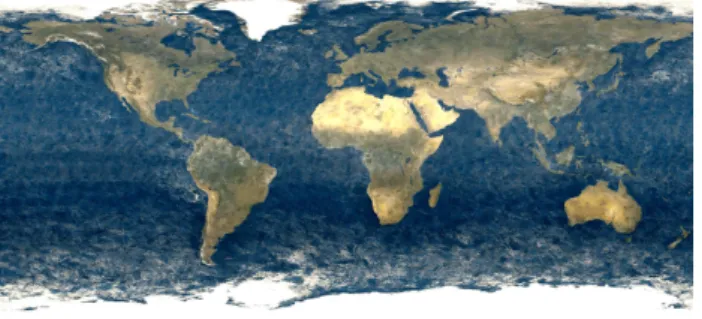
Fig. 2. Similar to Fig. 1, showing the Earth surface as seen by
SCIA-MACHY PMD 4, 5, and 6, as fake blue, green and red, respectively, during the months February and March 2003. The ice-caps and snowy northern latitudes show up in purple, while clouds appear green-grey.
PMD 2. In this way the most cloud-free possible colour im-age of the Earth is obtained. The imim-age shows that PMD 2, 3, and 4 can be used as broadband intensity measurements without a calibration for polarisation or viewing angle de-pendence.
A similar map can be made by applying the near-infrared PMDs. Figure 2 shows again the Earth surface, but now PMD 6, 5 and 4, are used linearly for red, green and blue respectively. This image is constructed using only February and March 2003 SCIAMACHY data, in order to clearly show the effects of winter (ice/snow) at the northern latitudes on the PMDs. Full cloud-free global coverage is therefore not achieved because of the shorter period. As such many clouds are still visible as green-grey patches, because at certain lo-cations no cloud-free observation was present during this pe-riod. However note the clear difference between clouds and ice/snow as clouds are a green-grey, but ice/snow shows up as clear purple at the Poles and the snowy northern high lat-itudes. A purple colour indicates a strong intensity in both “red” (PMD 6) and “blue” (PMD 4) and at the same time a low intensity in “green” (PMD 5). This difference will be ex-ploited to distinguish between clouds and ice/snow covered surfaces in Sect. 4.
3 Cloud recognition
3.1 SCIAMACHY PMD calibration
Clouds can easily be spotted in any visual Earth image from space, because in the visible wavelengths, clouds are bright and white whereas the background on which they appear is usually not. Obviously, this is not the case when there is snow or ice in the background, but these cases will be ad-dressed in the next section. Clouds are white in the visible wavelengths as they reflect all wavelengths equally yet ab-sorb little, because the water or ice particles of the cloud are
much larger than the wavelengths of the visual photons. This degree of “whiteness” can be used to detect the presence of clouds.
As SCIAMACHY PMDs are not absolutely calibrated, each SCIAMACHY PMD 2, 3 and 4 readout is first weighted or semi-calibrated. While each cloud will have a different reflectance (due to cloud fraction, type, altitude), the inten-sities in all three PMDs for each individual cloud should be similar, as clouds have a wavelength independent spectrum in the visible wavelength range (Bowker et al., 1985). The weighting factors were derived by selecting clouded scenes and normalising the readout distribution of PMD 2 and 4 to PMD 3 for these scenes. As mentioned before, PMD 1 is not used because of its strong polarisation sensitivity. The PMD signals are weighted as follows:
W4=SPMD 4/Ar W3=SPMD 3/Ag W2=SPMD 2/Ab,
(2)
where Ar, Ag, Ab are the weighting factors, 0.795, 1.000,
and 0.750, respectively, and W the weighted PMD read-out. These weighting factors have been derived for SCIA-MACHY processor version 5.04, but can be used on earlier versions, as the changes between versions, so far, in non-calibrated PMD measurements are less than a percent for the PMDs used by SPICI.
3.2 Saturation
The saturation or the “whiteness” for each observed scene can then be derived from these values as follows:
Saturation = max(W4, W3, W2) −min(W4, W3, W2) max(W4, W3, W2)
, (3) where max(W4, W3, W2)and min(W4, W3, W2)are,
respec-tively, the highest and lowest value of W4, W3, and W2 for
each simultaneous measurement. Saturation can vary be-tween 0–1 and will be low when all three PMDs are equally bright (= “white”) and high when the three PMD readouts differ much. For more details on the use of saturation in colour applications see Foley et al. (1990). Scenes with low saturation have thus a high “whiteness” which indicates a clouded scene (or snow covered surface). A threshold can then be determined for which all scenes with a saturation-value below this threshold are apparently clouded. A large advantage of using a saturation threshold instead of individ-ual PMD thresholds is that saturation is determined from a ratio between PMDs. In a ratio between PMDs the geome-try component is eliminated (Loyola, 1998) and as such no correction for solar zenith angle or viewing angle is needed. 3.3 MODIS
In order to derive the required saturation threshold SCIA-MACHY observations are compared to MODIS
(MODer-ate resolution Imaging Spectroradiometer) observations on-board the Terra (EOS AM) satellite. Terra is in a sun-synchronous, near-polar, descending orbit at 705 km and has an equator crossing time of 10:30 UT, only half an hour later than SCIAMACHY, making it useful for collocated compar-isons. Terra MODIS covers the entire Earth’s surface ev-ery 1 to 2 days, with a swath of 2330 km across track and 10 km along track (in nadir), with spatial resolution between 250 m×250 m and 5 km×5 km, depending on wavelength.
Several of the spectral bands are used for the MODIS Cloud Mask product which provides a daily global Level 2 data product at 1 km×1 km spatial resolution, which is used in this study. The MODIS algorithm (Ackerman et al., 2002) employs a combination of different tests on the visible and infrared channels to indicate various confidence levels that an unobstructed (= cloud-free) view of the Earth’s surface is observed. These tests are reflectance thresholds (for 0.66, 0.87, 1.38 µm), reflectance ratios (0.87/0.66 µm), brightness temperature thresholds (for 6.7, 11, 13.9 µm) and bright-ness temperature differences (between 11–6.7, 3.7–12, 8.6-11, 11–12 and, 11–3.9 µm). Also a spatial variability test has been included. MODIS detects clouds over ice/snow us-ing the brightness temperature at 6.7 and 13.9 µm, the bright-ness temperature differences between 11–6.7 and 11–3.9 µm and reflectances at 1.38, 0.66 and 0.87 µm.
The resulting MODIS cloud mask gives 4 possible confi-dence levels: confident clear (3), probably clear (2), probably cloudy (1), and confident cloudy (0). The probably clear and cloudy values are most often found at the edges of clouds, and indicate partially clouded scenes. The MODIS cloud de-tection algorithm has been extensively validated and appears to work very well in daylight conditions. Nighttime observa-tions, however, are still problematic (Ackerman et al., 20051, private communication, 2005). In this study only daytime observations are used because MODIS observations are com-pared with collocated SCIAMACHY daytime observations. Therefore the MODIS cloud mask data is used to develop and validate the SPICI algorithm applied to SCIAMACHY data.
As the MODIS footprint (1 km×1 km) is much smaller than the SCIAMACHY PMD footprint (7 km×30 km), all MODIS observations that fall within a single SCIAMACHY PMD observation are combined and their cloud values (be-tween 0 and 3) are averaged. On average be(be-tween 100 and 250 MODIS footprints fall within a single SCIAMACHY PMD footprint. In the remainder of this study we re-fer to PMD observations with an average MODIS cloud value above 2.95 as “clear” and with a value below 0.05 as “clouded”. To illustrate that this is a rather strict clas-sification one should realise that a value of 2.95 represents for example a maximum of ∼2 MODIS cloudy observations and ∼98 MODIS cloud-free observations in the collocated
1Ackerman et al.: MODIS Cloud mask validation, in
J. M. Krijger et al.: SCIAMACHY PMDs Identification of Clouds and Ice/snow 2733
Fig. 3. Comparison between saturation-value of SCIAMACHY
PMD observations that are either “clouded” (black), “clear” (blue) or mixed (red) according to collocated MODIS data averaged over the SCIAMACHY PMD footprint. Observations are over Europe and Africe on 16 June 2004.
SCIAMACHY observation corresponding to a cloud-fraction of maximal 0.02.
3.4 Threshold determination
These average MODIS cloud values over a SCIAMACHY PMD observation can be compared to the saturation-value S for each individual PMD observation. For this, collocated observations (lat. 14◦–55◦N, long. 7◦W–18◦E) of SCIA-MACHY (∼10:15 UT) and MODIS (∼10:50 UT) on 16 June 2004 over Europe and Africa were compared. The selected region avoids ice/snow covered areas. Figure 3 shows the number of SCIAMACHY PMD observations with a partic-ular saturation or “whiteness” for “clouded”, “clear” and all remaining (mixed) scenes according to the MODIS data. The “clouded” and “clear” curves show two clearly distinct distri-butions in saturation-value, indicating that this parameter can be used to differentiate between clouded and clear scenes. Observations which are partly clouded show more variation in saturation-value, because an average of the “clouded” and “clear” scenes is found. As we want to keep the number of mistakenly flagged cloud-free observations to a minimum, we use a threshold saturation-value of 0.35 in the remainder of the study. However for studies focusing on clouds (instead of clear scenes) or where an occasional cloud is not a prob-lem a threshold of 0.25 can be used, increasing the number of detected “clear” scenes.
3.5 Spatial comparison MODIS–SPICI
Figure 4 shows the spatial comparison between the used SCIAMACHY (∼10:15 UT) and MODIS (∼10:50 UT) ob-servations on 16 June 2004. All SCIAMACHY PMD obser-vations with a saturation below 0.35 are indicated as clouded, those with a higher saturation-value as clear. The colours
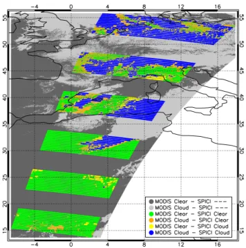
Fig. 4. Comparison between SCIAMACHY (∼10:15 UT) SPICI
and MODIS (∼10:50 UT) observations on 16 June 2004 (same as used in Fig. 3). The legend indicates the colours used for all pos-sible different (dis)agreements between MODIS (lefthand-side of legend) and SCIAMACHY SPICI (righthand-side). Note that the plotted MODIS observations are at 1 km×1 km resolution while the SCIAMACHY observations are ∼7 km×30 km.
indicate where the methods agree (blue, green) or disagree (orange, yellow). The agreement is very good, only in a few cases there is a disagreement. The most troubling dis-agreements are when MODIS indicates a (maybe) cloud, while SCIAMACHY PMD saturation-value indicates a clear scene. These cases only occur at the edge of clouds, likely due to movement (or formation) of clouds in the 35 min in-between the observations. For example, around 5◦
longi-tude and 32◦latitude a cloud apparently moved to the east,
as SCIAMACHY indicates clear scenes on the east of the cloud while MODIS (35 min later) indicates these scenes as clouded. On the west side of the cloud the reverse happens, confirming that the cloud moved to the east. Also the cloud cover over northern Europe for this morning is extremely patchy, resulting in some disagreements between MODIS and SCIAMACHY cloud identification. It is noted that all mixed scenes from Fig. 3 coincide with these cloud edges.
The above cloud detection scheme is based upon the “whiteness” – in the visible wavelength range – of the scene, and therefore does not distinguish between clouds and ice/snow covered surfaces. This is a problem for many cloud detection algorithms, but SCIAMACHY’s infra-red PMDs allow for differentiating between clouds and ice/snow cov-ered surfaces as shown in the next section.
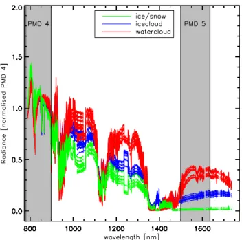
Fig. 5. Comparison between spectral behaviour of several
water-clouds (red), ice-water-clouds (blue) and snow (green) scenes as mea-sured by SCIAMACHY (over Greenland during 30 June 2002). The wavelength ranges of PMD 4 and 5 are indicated. The mea-surements are normalised to the PMD 4 wavelength range. Both type of clouds are much brighter relative to snow at PMD 5 wave-lengths. Jumps in the spectrum around 1050 and 1250 nm are due to spatial variation during different integration-times between various wavelength-ranges as employed by SCIAMACHY.
4 Ice recognition
4.1 Physical background
All existing cloud detection algorithms using PMDs are de-rived from GOME algorithms, which are unable to distin-guish between white ice/snow and white clouds because the GOME wavelength range is limited to 800 nm. However SCIAMACHY infra-red PMDs allow for differentiation be-tween clouds and ice/snow covered surfaces.
Several kinds of clouds exists: water clouds, ice clouds and mixed-phase clouds. In the infra-red region around 1.6 µm, which corresponds to the wavelength range covered by PMD 5, water and ice have a distinctly different refractive in-dex (Kokhanovsky, 2004). The imaginary part of the refrac-tive index, which determines the absorption, is much larger for ice than water. In addition, it is noted that water and ice show very different spectral absorption features around 1.6 µm which can be used for cloud phase discrimination as was shown by Knap et al. (2002) and Acarreta et al. (2004) using SCIAMACHY measurements.
Ice/snow covered surfaces are dark compared to water clouds (Bowker et al., 1985), due to the larger imaginary
re-fractive index around 1.6 µm and the larger effective particle radius of an ice/snow covered surface (Wiscombe and War-ren, 1980; WarWar-ren, 1982). This is also observed in SCIA-MACHY spectra (Fig. 5) measured with the main spectrom-eter where a clear difference is visible between a water cloud and ice/snow covered surface.
Clouds, however, can also consist of ice particles with a refractive index comparable to ice on the Earth’s surface, which might limit the possibility to distinguish between ice clouds and ice/snow covered surfaces. However, ice clouds have an effective particle radius still much smaller com-pared to ice/snow (e.g., around 15 µm comcom-pared to possi-bly 200 µm), therefore ice clouds show less absorption com-pared to ice/snow covered surfaces (Wiscombe and Warren, 1980; Warren, 1982). This is illustrated in Fig. 5 (ice cloud) where the MODIS identification of ice clouds (Platnick et al., 2003) is used to select the corresponding SCIAMACHY ice cloud spectrum. Figure 5 further shows that ice cloud spec-tra can be considered an intermediate case between the bright water cloud spectra and dark ice/snow surface spectra. The difference in reflectance between ice clouds and ice/snow covered surface around 1.6 µm is large enough to distinguish these in most cases (Crane and Anderson, 1984).
While changing the optical thickness of the cloud, com-pacting the ice/snow or changing the amount of dirt mixed with the ice/snow does change the reflectance, the large dif-ference in reflectance around 1.6 µm between (ice and water) clouds and ice/snow remains (Kokhanovsky, 2004; Greuell and Oerlemans, 2004). This difference in absorption at 1.6 µm, and measured with PMD 5, is used in the SPICI al-gorithm to distinguish between (water and ice) clouds and ice/snow covered surfaces.
In order to further improve the differentiation between (ice and water) clouds and ice/snow covered surfaces, the PMD 5 measurements around 1.6 µm are normalised with the PMD 4 measurements around 850 nm. The reflectance around 850 nm is larger for ice/snow covered surfaces than (water or ice) clouds contrary to what is observed at 1.6 µm enhancing the relative difference (Bowker et al., 1985). In addition, by taking the ratio of PMDs no correction for solar zenith angle or viewing angle is needed (Loyola, 1998). Tak-ing the ratio of PMD 5 with PMD 4 thus improves the dif-ferentiation between (ice and water) clouds and ice. While it should also be possible to use PMD 6 for this purpose, PMD 6 suffers from a very low signal-to-noise ratio, making it unsuitable for use in SPICI.
4.2 Threshold determination
The preferred approach would be to compare the expected ratio for PMD 5 and PMD 4 from theory with the measured ratio between PMD 5 and PMD 4. However, the required ab-solute calibration of SCIAMACHY PMDs is lacking. There-fore the threshold for the PMD 5 to 4 ratio to differentiate
J. M. Krijger et al.: SCIAMACHY PMDs Identification of Clouds and Ice/snow 2735
Fig. 6. Number of occurrences of certain ratios between PMD 5 and
PMD 4 for “clouded” (black), “clear” (blue) and mixed (red) scenes according to MODIS over Antartica on 24 January 2003.
between clouds and ice/snow surfaces is empirically deter-mined using collocated MODIS observations.
Collocated MODIS and SCIAMACHY observations are used, this time observed over Antarctica on 24 January 2003 between 08:30–09:10 UT by SCIAMACHY and at 08:50 UT by MODIS. As in the previous section all MODIS obser-vations within a single PMD observation are averaged for comparison. Figure 6 shows the number of SCIAMACHY PMD observations with a particular ratio between PMD 5 and PMD 4 for “clouded” and “clear” scenes according to averaged collocated MODIS data. As the observations are over Antarctica all “clear” scenes are observing snow or ice surfaces. The “clouded” and “clear” curves show two clearly distinct distributions, indicating that the ratio tween PMD 5 and PMD 4 can be used to differentiate be-tween clouds and ice/snow covered surfaces. Most PMD observations with a ratio SPMD 5/SPMD 4 below 0.4 appear
to be ice/snow covered surfaces. In general, however, most SCIAMACHY observations occur over more diverse scenes than only ice/snow covered surfaces and clouds as here over Antarctica. The ratios of other scenes can vary and must therefore be verified, as care must be taken not to mistakenly identify clouds as ice/snow covered surfaces.
Figure 7 shows the number of SCIAMACHY PMD ob-servations as a function of the ratio between PMD 5 and PMD 4 for “clouded” and “clear” scenes according to aver-aged collocated MODIS data for the scene over Europe and Africa in the previous section. Most “clear” scenes (observ-ing sea, desert and vegetation) have a high SPMD 5/SPMD 4
ratio around 1.8, but we see a different distribution for the “clouded” scenes, varying mostly between 0.2 and 1.2. How-ever, in these particular observations we expect to find little ice/snow covered surfaces as the observations were made in mid-summer June. If here a threshold of 0.4 was used several clouds would have been -mistakenly- identified as ice/snow covered surfaces. Therefore, a lower limit than 0.4 for the
ra-Fig. 7. Number of occurrences of certain ratios between PMD 5 and
PMD 4 for “clouded” (black), “clear” (blue) and mixed (red) scenes according to MODIS over Europe and Africa on 16 June 2004.
Fig. 8. Number of occurrences of certain ratios between PMD 5 and
PMD 4 over Europe on 23 August 2002.
tio SPMD 5/SPMD 4must be used. Figure 7 suggests a value of
0.2, but studying ratios over several other SCIAMACHY or-bits in the summer, shows that the lower limit for cloudy ob-servations in the ratio is around 0.16, as illustrated in Fig. 8, which shows the SCIAMACHY data for 2 orbits on 23 Au-gust 2002, over western Europe and the Atlantic ocean, con-taining no ice/snow covered surfaces. No comparison with MODIS was made for this data, so no distinction is made between “clouded” and “clear” scenes, but when comparing to the ratios from 16 June 2004 (Fig. 7), the similarity in the distributions is clear. In order to avoid mistakenly identifying clouds as ice/snow, we choose a ratio between PMD 5 and PMD 4 of 0.16 to distinguish between cloud-free ice/snow covered surfaces and clouds, knowingly overestimating the amount of clouds compared to cloud-free ice/snow scenes. For observations over Antarctica or studies less sensitive to clouds a larger ratio up to 0.4 can be chosen.
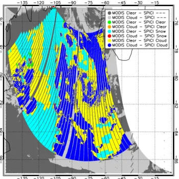
Fig. 9. Comparison between clouds and ice/snow observations as
identified by SCIAMACHY (08:30–09:10 UT) SPICI and MODIS (08:50 UT) on 24 January 2003 over Antartica, colour-coded as in-dicated in the legend.
4.3 Spatial comparison MODIS-SPICI
Figure 9 allows a spatial comparison between the used SCIA-MACHY (08:30–09:10 UT) and MODIS (08:50 UT) ob-servations on 24 January 2003 over Antarctica. All SCIA-MACHY PMD observations with a saturation-value below 0.35 are indicated clouded, and those with a higher saturation as clear. In the next step, all indicated clouded scenes with a ratio between PMD 5 and PMD 4 below 0.16 are re-assigned as ice/snow covered surfaces. The legend indicates where the methods agree or disagree. The only notable disagreement is when a SCIAMACHY PMD observation is identified as clouded whereas MODIS assigned clear (yellow). In the east part the number of clouds is thus overestimated by SCIA-MACHY compared to MODIS, but this is to be expected due to the low ratio (0.16 instead of 0.4) used for differentiat-ing between ice/snow and clouds. For our purpose the most troubling disagreements would be where MODIS indicates a cloud, while SCIAMACHY PMD saturation-value indicates a clear ice/snow scene (red). Only in a few single cases this happens at the (western) edges of the central cloud complex, likely due to movement of the clouds in the time in-between the observations. Also SCIAMACHY indicates a few single scenes as being clear (green), while over the Antarctica all clear scenes should show ice/snow. However for the purpose of removing clouded scenes this is not relevant.
Fig. 10. Similar to Fig. 9, but now showing results over
Green-land, the Atlantic Ocean and Eastern Canada. Comparison between SCIAMACHY (13:48–14:12 UT) SPICI and MODIS (14:40 UT) on 30 June 2002, colour-coded as indicated in the legend.
5 Method validation
In order to validate the SPICI method a final comparison was made between SCIAMACHY (13:48–14:12 UT) and collo-cated MODIS (14:40 UT) data observed on 30 June 2002. These observations are partly over Greenland, the Atlantic Ocean and eastern Canada, combining clouded, clear and ice/snow scenes within the same orbit. This allows a di-rect validation of the SPICI method as presented in the previ-ous sections. Again all MODIS observations within a single PMD observation are averaged. Figure 10 shows the spatial comparison. Again the agreement is very good. Over Green-land ice/snow scenes are indicated where the sky is clear according to MODIS (light blue), while over the ocean the SPICI method indicated normally clear (green) or clouded (dark blue) skies at the exact same locations as MODIS. Only a few single/individual disagreements (red, orange) show-up, all occurring at the edge of large cloud complexes or over patchy cloud regions. Again most likely this is due the move-ment of the clouds in the time between the SCIAMACHY and MODIS observations.
A more quantitative comparison between SPICI and MODIS is summarised in Table 2 where the number of obser-vations for the different (dis)agreements are shown. As such a total of 7552 SPICI observations with collocated MODIS observations were used. Of these 48% (3615) were confi-dently clouded (“clouded”), 14% (1060) were conficonfi-dently
J. M. Krijger et al.: SCIAMACHY PMDs Identification of Clouds and Ice/snow 2737
Table 2. Number of PMD observations for different agreements
between MODIS and SPICI for 30 June 2002.
SPICI MODIS counts
All All 7552 Cloud Cloud 3479 Cloud Clear 143 Cloud Mixed∗ 1781 Clear Cloud 136 Clear Clear 917 Clear Mixed∗ 1096 ∗
Mixed refers to neither confidently clear, nor confidently clouded.
clear (“clear”), and 38% (2877) were neither confidently clear nor confidently clouded (“mixed”). We focus on the “clouded” and “clear” observations. As SPICI has been tuned such that cloudy observations are rarely flagged cloud-free, the most important comparison is with the observa-tions that are ’clouded’ according to MODIS. When includ-ing ice/snow covered surfaces accordinclud-ing to SPICI as clear, SPICI identifies 96% of the MODIS “clouded” observations as clouded and only 4% is mistakenly identified as clear. The next important comparison is the observations that are “clear” according to MODIS while SPICI mistakenly labels them clouded. These observations will often not be used and as such should preferably be kept to a minimum. As such, SPICI identifies 87% of the MODIS “clear” as clear and only 13% of the MODIS “clear” observations as clouded. By choosing different thresholds these percentages can vary, but it can be concluded that current thresholds minimise cloud-contamination in the SPICI clear observations, with an ac-ceptable amount of cloud-free observations mislabelled as clouded. All this combined shows the very good agreement between MODIS and SPICI.
6 Summary
For the accurate detection of well-mixed tropospheric gasses, such as CH4and CO2, the use of cloud-free observations is
extremely important. The slightest cloud-contamination af-fects the quality of these data products which could make them useless. In this paper the SPICI method is presented which allows for fast and simple identification of cloud-free SCIAMACHY PMD observations. The NIR SCIAMACHY PMD measurements allow to distinguish between clouds and ice/snow covered surfaces, which in the visible wavelengths is more complicated. The method employs the ratios of dif-ferent SCIAMACHY PMD measurements which makes the approach very robust with respect to e.g. calibration uncer-tainties. The threshold values are defined using collocated observations with the well known and validated high-spatial resolution MODIS data. The threshold values are tuned such
that cloudy observations are rarely flagged cloud-free, as such some cloud-free observations are mistakenly flagged cloudy. Clearly, one can use the SPICI algorithm and adjust the criteria depending on the use of the data.
The SPICI method is very easily implemented, requiring only a few numbers. For those studies that require cloud-free scenes these are summarised as follows:
W4 =SPMD4/0.795
W3 =SPMD3/1.000
W2 =SPMD2/0.750
Sat(uration) = max(W4,W3,W2)−min(W4,W3,W2) max(W4,W3,W2)
Cloud−free : Sat ≥ 0.35
Ice/Snow clear : Sat < 0.35 &SPMD 5
SPMD 4 ≤0.16
Cloud : Sat < 0.35 &SPMD 5
SPMD 4 ≥0.16
(4)
The thresholds can be somewhat relaxed in cases where some cloud-contamination is acceptable.
Acknowledgements. We would like to thank A. Maurellis, J.
Skid-more, and W. Hartmann for their comments, R. van Hees for his software codes and the anonymous referees for their comments. Financial support is acknowledged from NIVR (SCIAMACHY phase E). ESA is acknowledged for providing SCIAMACHY data (@ESA 1995–1996) processed by DFD/DLR, Esrin/ESA. The MODIS data used in this study were acquired as part of the NASA’s Earth Science Enterprise. The algorithms were developed by the MODIS Science Teams. The data were processed by the MODIS Adaptive Processing System (MODAPS) and Goddard Distributed Active Archive Center (DAAC), and are archived and distributed by the Goddard DAAC.
Edited by: H. Kelder
References
Acarreta, J. R., Stammes, P., and Knap, W. H.: First retrieval of cloud phase from SCIAMACHY spectra around 1.6 micron, At-mos. Res., 72, 89–105, 2004.
Ackerman, S. A., Strabala, K. I., Menzel, W. P., Frey, R. A., Moeller, C. C., Gumley, L. E., Baum, B., Wetzel-Seeman, S., and Zhang, H.: Discriminating clear sky from clouds with MODIS Algorithm Theoritical Basis Document (MOD35), 2002. Bovensmann, H., Burrows, J. P., Buchwitz, M., Frerick, J., Noel, S.,
Rozanov, V. V., Chance, K. V., and Goede, A. P. H.: Sciamachy: Mission objectives and measurement modes, J. Atmos. Sci., 56, 127–150, 1999.
Bowker, D., Davis, R., Myrick, D., Stacy, K., and Jones, W.: Spec-tral reflectances of natural targets for use in remote sensing stud-ies, NASA Reference Publication 1139, 1985.
Burrows, J. P., Weber, M., Buchwitz, M., Rozanov, V., Ladst¨atter-Weißenmayer, A., Richter, A., Debeek, R., Hoogen, R., Bramst-edt, K., Eichmann, K., Eisinger, M., and Perner, D.: The Global Ozone Monitoring Experiment (GOME): Mission Concept and First Scientific Results., J. Atmos. Sci., 56, 151–175, 1999.
Crane, R. G. and Anderson, M. R.: Satellite discrimination of snow/cloud surfaces, Int. J. Remote Sensing, 5, 1984.
Foley, J., van Dam, A., Feiner, S., and Hughes, J.: Computer Graph-ics: Principles and Practice, Addison-Wesley, 1990.
Greuell, W. and Oerlemans, J.: Narrowband-to-broadband albedo conversion for glacier ice and snow: equations based on mod-elling and ranges of validity of the equations, Rem. Sens. Envi-ron., 89, 95–105, 2004.
Grzegorski, M., Frankenburg, C., Plat, U., Wenig, M., Fournier, N., Stammes, P., and Wagner, T.: Determination of cloud parame-ters from SCIAMACHY data for the correction of tropospheric trace gases, in Proceedings of the ENVISAT & ERS Sympo-sium, 6–10 Septembeer 2004, Salzburg, Austria, ESA Publica-tion SP-572, (CD-ROM), 2004.
Knap, W. H., Stammes, P., and Koelemeijer, R. B. A.: Cloud thermodynamic-phase determination from near-infrared spectra of reflected sunlight, J. Atmos. Sci., 59, 83–96, 2002.
Koelemeijer, R. B. A., Stammes, P., Hovenier, J. W., and de Haan, J. F.: A fast method for retrieval of cloud parameters using oxy-gen A band measurements from the Global Ozone Monitoring Experiment, J. Geophys. Res., 15, 3475–3490, 2001.
Kokhanovsky, A.: Optical properties of terrestial clouds, Earth-Science Reviews, 64, 189–241, 2004.
Kurosu, T. P., Chance, K., and Spurr, R. J. D.: Cloud Retrieval Al-gorithm for the European Space Agency’s Global Ozone Mon-itoring Experiment, Proceedings of SPIE, EUROPTO Series: Satellite Remote Sensing of Clouds and the Atmosphere III, edited by: Russel, J. E., 495, 17–26, 1998.
Kuze, A. and Chance, K. V.: Analysis of cloud top height and cloud coverage from satellites using the O2A and B bands, J. Geophys.
Res., 99, 14 481–14 491, 1994.
Loyola, D.: A New Cloud Recognition Algorithm for Optical Sen-sors, in: IEEE International Geoscience and Remote Sensing Symposium, Vol. 2 of IGARSS 1998 Digest, 572–574, 1998. Mahesh, A., Gray, M. A., Palm, S. P., Hart, W. D., and Spinhirne,
J. D.: Passive and active detection of clouds: Comparisons be-tween MODIS and GLAS observations, Geophys. Res. Lett., 31, 4108, doi:10.1029/2003GL018859, 2004.
Platnick, S., King, M. D., Ackerman, S. A., Menzel, W. P., Baum, B. A., and Ridi, J. C., and Frey, R. A.: The MODIS Cloud Prod-ucts: Algorithms and Examples from Terra, IEEE Transactions on Geoscience and Remote Sensing, 41, 459–473, 2003. Rozanov, V. V. and Kokhanovsky, A. A.: Semianalytical cloud
re-trieval algorithm as applied to the cloud top altitude and the cloud geometrical thickness determination from top-of-atmosphere re-flectance measurements in the oxygen A band, J. Geophys. Res.-Atmos., 109, D5202, doi:10.1029/2003JD004104, 2004. Slijkhuis, S.: ENVISAT-1 SCIAMACHY level 0 to 1c processing,
algorithm theoretical basis document, issue 2 (ENV-ATB-DLR-SCIA-0041), Tech. rep., DLR, 2000.
von Bargen, A., Kurosu, T., Chance, K., Loyola, D., Aberle, B., and Spurr, R. J.: Cloud retrieval algorithm for gome (crag), Report ER-TN-DKLR-CRAG-007, European Space Agency (ESA/ESTEC), Noordwijk, 2000.
Warren, S. G.: Optical properties of snow, Rev. Gephys. Space Phys., 20, 67–89, 1982.
Wenig, M.: Satellite Measurements of Long-Term Global Tropo-spheric Trace Gas Distributions and Source Strengths, PhD the-sis, University of Heidelberg, Germany, 2001.
Wiscombe, W. J. and Warren, S. G.: A model for the specrtal albedo of snow. I. Pure Snow, J. Atmos. Sci., 37, 2712–2733, 1980.