HAL Id: hal-00318412
https://hal.archives-ouvertes.fr/hal-00318412
Submitted on 29 Nov 2007
HAL is a multi-disciplinary open access
archive for the deposit and dissemination of
sci-entific research documents, whether they are
pub-lished or not. The documents may come from
teaching and research institutions in France or
abroad, or from public or private research centers.
L’archive ouverte pluridisciplinaire HAL, est
destinée au dépôt et à la diffusion de documents
scientifiques de niveau recherche, publiés ou non,
émanant des établissements d’enseignement et de
recherche français ou étrangers, des laboratoires
publics ou privés.
Cluster
T. Johansson, G. Marklund, T. Karlsson, S. Liléo, P.-A. Lindqvist, Hans
Nilsson, S. Buchert
To cite this version:
T. Johansson, G. Marklund, T. Karlsson, S. Liléo, P.-A. Lindqvist, et al.. Scale sizes of intense auroral
electric fields observed by Cluster. Annales Geophysicae, European Geosciences Union, 2007, 25 (11),
pp.2413-2425. �hal-00318412�
www.ann-geophys.net/25/2413/2007/ © European Geosciences Union 2007
Annales
Geophysicae
Scale sizes of intense auroral electric fields observed by Cluster
T. Johansson1, G. Marklund1, T. Karlsson1, S. Lil´eo1, P.-A. Lindqvist1, H. Nilsson2, and S. Buchert3
1Space and Plasma Physics, School of Electrical Engineering, Royal Institute of Technology (KTH), Stockholm, Sweden 2Swedish Institute of Space Physics, Kiruna, Sweden
3Swedish Institute of Space Physics, Uppsala, Sweden
Received: 4 June 2007 – Revised: 17 October 2007 – Accepted: 30 October 2007 – Published: 29 November 2007
Abstract. The scale sizes of intense (>0.15 V/m, mapped to
the ionosphere), high-altitude (4–7 RE geocentric distance)
auroral electric fields (measured by the Cluster EFW instru-ment) have been determined in a statistical study. Monopo-lar and bipoMonopo-lar electric fields, and converging and diverging events, are separated. The relations between the scale size, the intensity and the potential variation are investigated.
The electric field scale sizes are further compared with the scale sizes and widths of the associated field-aligned currents (FACs). The influence of, or relation between, other param-eters (proton gyroradius, plasma density gradients, and geo-magnetic activity), and the electric field scale sizes are con-sidered.
The median scale sizes of these auroral electric field struc-tures are found to be similar to the median scale sizes of the associated FACs and the density gradients (all in the range 4.2–4.9 km) but not to the median proton gyroradius or the proton inertial scale length at these times and locations (22– 30 km). (The scales are mapped to the ionospheric altitude for reference.)
The electric field scale sizes during summer months and high geomagnetic activity (Kp>3) are typically 2–3 km,
smaller than the typical 4–5 km scale sizes during winter months and low geomagnetic activity (Kp≤3), indicating a
dependence on ionospheric conductivity.
Keywords. Magnetospheric Physics (auroral phenomena;
electric fields; magnetosphere-ionosphere interactions)
Correspondence to: T. Johansson ([email protected])
1 Introduction
Intense quasi-static auroral electric fields have been observed by Cluster in both the upward current region (Vaivads et al., 2003; Figueiredo et al., 2005) and the downward current re-gion (Marklund et al., 2001; Johansson et al., 2004). The associated potential structures can be either S-shaped or U-shaped, corresponding to monopolar and bipolar electric field signatures, respectively. Both types have been observed and the S-shaped potential structures have been shown to be associated with the sharp plasma density gradient at the plasma sheet boundary, while U-shaped potential structures occur inside the plasma sheet at less distinct gradients (Jo-hansson et al., 2006; Marklund et al., 2007). These electric fields have a component parallel to the magnetic field, accel-erating particles upward and downward. Theories attempt-ing to explain parallel the electric fields include, e.g., strong double layers (Block, 1972), weak double layers (Temerin et al., 1982), Alfv´en waves (Song and Lysak, 2001), anoma-lous resistivity (Hudson and Mozer, 1978) and magnetic mir-ror supported fields (Knight, 1973; Chiu and Schulz, 1978). Temerin and Carlson (1998) discussed the current-voltage re-lation in the downward FAC region and presented a model based on average charge neutrality but with the possibility of contribution to the parallel electric field from anomalous re-sistivity. Jasperse (1998) described downward parallel elec-tric fields in a kinetic model, and Jasperse and Grossbard (2000) developed an analogue to the Alfv´en-F¨althammar for-mula for the downward current region.
There are several spatial scales associated with auroral ac-tivity: fine-scale auroral arcs (order of 100 m), arc systems (order of 1 km) and the thickness of the auroral zone (order of 100 km) (Borovsky, 1993; Galperin, 2002). In a review of 21 theories attempting to describe the formation of au-roral arcs, Borovsky (1993) found that none of them could predict arc widths of some 100 m, which was the average of the thickness of the auroral structures observed by Maggs
and Davis (1968). Several theories gave arc thicknesses of a few km at ionospheric altitude (e.g., strong double layers and anomalous resistivity) but some gave scale sizes one or two order of magnitudes larger than that. McFadden et al. (1999) presented a scenario (based on FAST observations of electric field structures), in which the quasi-static potential structures consist of narrow structures extending to low altitudes. How-ever, these narrower structures were a few km wide, still an order of magnitude larger than the fine-scale auroral arcs.
In a statistical study of optically observed stable mesoscale auroral arcs, Knudsen et al. (2001) found a mean width of 18 km, with a sharp cutoff at 8 km. Together with the re-sults of Maggs and Davis (1968), this leaves a gap in the auroral arc width distribution near 1 km (see Fig. 4 in Knud-sen et al. (2001)). This might mean that there are different mechanisms for the fine-scale arcs and the mesoscale arcs, although uncertainties in the measurement resolution can not be ruled out as the cause of this gap.
Stenbaek-Nielsen et al. (1998) reported on optical obser-vations showing arc widths down to 2 km, similar to the size of auroral structures inferred from conjugate FAST electron energy flux measurements. This implies that the processes determining the arc widths at this scale occur at or above the FAST altitude of ∼4000 km.
Diverging bipolar electric fields accelerate electrons up-ward in the downup-ward current and they have been suggested to correspond to black aurora (Marklund et al., 1997). How-ever, in a study using optical and radar measurements, Blixt and Kosch (2004) did not find electron density depletions for two events of black aurora, which would be expected for a downward FAC driven by a intense diverging electric field. The 1–2 km wide black arcs were surrounded by diffuse au-rora. Peticolas et al. (2002) found only small electric fields (<10 mV/m) associated with black aurora in a study of FAST particle data (the electron signature was a ∼3 km wide en-ergy flux depletion region) and conjugate aircraft-based opti-cal measurements. The surrounding bright aurora was mostly diffuse. More intense electric fields associated with black au-rora were found by Kimball and Hallinan (1998). Using the vorticity of four observed black curls, they could estimate the electric fields to be 80 to 300 mV/m. These black curls were found together with white curls. It is possible that the intense diverging electric fields associated with the downward cur-rent region only occur for black auroras found together with discrete bright arcs (intense upward current), while there is no need for such intense electric fields for black aurora resid-ing within diffuse white aurora.
In a statistical study of black aurora, Trondsen and Cog-ger (1997) found black aurora objects (black patches and arc segments) with scale sizes of 0.5–1.5 km. Black auro-ral arcs were found to have scale sizes in the range 200 m to 1 km with a preferred thickness of 400–500 m. The aver-age width of black auroral arcs, 615 m, were similar to the average (740 m) of the widths of bright auroral structures re-ported by Maggs and Davis (1968).
Karlsson and Marklund (1996) observed intense elec-tric fields, assumed to be diverging, at low altitude (1400– 1770 km) and found that their scale sizes were inversely pro-portional to the intensities of the electric fields, with the most intense electric fields being those with the smallest scale size. The typical scale size of the most intense of these electric field structures was 1–5 km. This inverse relation was also found in a Cluster study (Johansson et al., 2005), includ-ing both converginclud-ing and diverginclud-ing electric fields. An inverse proportionality has also been found between the scale size and intensity of FACs in the auroral region (Stasiewicz and Potemra, 1998). The most intense current magnitudes were found for the the smallest ∼100 m sized currents, and the in-tensity dropped with increasing scale size up to the largest FAC widths (∼500 km).
Alfv´en waves are also capable of accelerating electrons and powering the aurora, as shown by, e.g., Keiling et al. (2003). Chaston et al. (2003) discussed Alfv´en wave driven arcs. The widths of those arcs were of the order of 1 km at ionospheric altitude. Smaller arcs could possibly be pro-duced but they would have a too low intensity to explain the arcs of some 100 m observed by Maggs and Davis (1968). In a statistical study of upward accelerated electrons, An-dersson and Ergun (2006) found good agreement between the electric field measurements and the characteristic energy of electrons in 50 percent of the events, consistent with the quasi-static model. Andersson and Ergun (2006) speculated that the poor correlation for the other half of the events might be due to Alfv´en wave acceleration of the electrons. An-other explanation would be that the electric field sometimes partly extends down to the ionosphere, giving a mismatch be-tween the measured electric field and the up-going electrons. Examples of this have been found by Hwang et al. (2006). In a study of downward electron acceleration, Newell et al. (1996) found, using the DMSP satellites, that the widths of such regions had a exponential distribution with a character-istic width of 28–35 km.
In this study, the scale sizes, S(E), of 797 intense au-roral electric field structures observed by the Cluster satel-lites at geocentric distances of 4–7 REare calculated together
with the scale sizes of the associated field-aligned currents, S(FAC), and density gradients, S(dn). The electric field scale sizes are investigated with respect to various condi-tions (e.g. summer/winter) and in relation to S(FAC), S(dn) and other plasma parameters. Monopolar electric fields (S-shaped potential structures) and bipolar electric fields (U-shaped potential structures) have been identified and, for the latter ones, a determination of whether they are diverging or converging has been conducted.
2 Method
The electric fields investigated in this statistical study were measured by the Cluster EFW instrument (Gustafsson et al.,
1997). A database was created by selecting events at geo-centric distances between 4 and 7 RE where the magnitude
of the electric fields, when mapped to ionosphere, exceeded 0.15 V/m. This database was also used by Johansson et al. (2005) in a study of the characteristics and occurrence of in-tense high-altitude electric fields. A total of 797 events have been used in this study. For each of the events, S(E) was calculated as the full-width half-maximum of the peak value. This rather simple method was also used by Karlsson and Marklund (1996) and also in other types of scale size de-terminations (e.g. Knudsen et al., 2001). The differences in definitions of scale sizes and type of measurement must be kept in mind when the results are compared.
The potential is calculated over a region proportional to the scale size, S(E), by integrating the perpendicular (to the background magnetic field) electric field. Then a smaller re-gion (still proportional to S(E)) is extracted. The first point in this new, shorter interval is chosen as reference point (zero level). Different types of electric fields have been separated by applying criteria to the potential. The potential signature of a monopolar electric field is a step, while converging and diverging electric fields are associated with negative (“val-ley”) and positive (“hill”) signatures in the potential, respec-tively. By comparing the potential (calculated from the elec-tric field) mid-value and start and end values in a region cen-tered at the electric field peak, the criteria could be checked automatically. An event where the mid-value of the potential is greater (smaller) than the start value but smaller (greater) than the end value has been labelled monopolar. If the mid-value is greater (smaller) than both start and end mid-values, the event has been labelled diverging (converging) bipolar. The potential variation across the structure has been determined as the maximum or minimum value for bipolar events and as the end value of the shorter region for monopolar events.
A fourth degree polynomial was fitted to the magnetic field measured by the FGM instrument (Balogh et al., 1997) and removed from the measured value. From the residual mag-netic field, and using the infinite current sheet approximation, the FACs associated with the electric field structures were calculated. The scale sizes S(FAC) have also been calculated as the full-width half-maximum of the current magnitude at the time of the event. The width of the current region, deter-mined as the region with the same current direction as at the time of the event, has been used as an alternative to S(FAC). The electric fields studied have been found to be colocated with density gradients, which are important for the shape of the associated potential structure (Johansson et al., 2006). The spatial scale used in this study to characterize the den-sity gradients is the scale size of the denden-sity gradient, S(dn). Note that S(dn) is not the scale size of a peak in the density. Using CIS ion data (R`eme et al., 1997), the gradient in the density was calculated and the maximum value of the density gradient associated with the electric field event was found. S(dn) was then determined as the full-width half-maximum of that peak in the density gradient. The proton gyroradius
and inertial scale length have also been calculated. Note that there are no CIS data available from Cluster 2.
The time resolution of the EFW instrument is, in normal mode, 0.04 s and the spatial resolution at ionospheric alti-tudes will be 0.015 km for measurements at 5 REgeocentric
distance. The CIS instrument has a time resolution of 4 s giving mapped spatial resolutions of 0.8–2.0 km for the geo-centric distances in this study (4–7 RE). The FGM magnetic
field data used have a spin resolution, same as the CIS instru-ment.
The electric field magnitudes and the spatial scales have been mapped to the ionospheric altitude for reference using the dipole magnetic field approximation. The mapping to the equator in Fig. 4 has been done using the same approxima-tion (Mozer, 1970; Weimer and Gurnett, 1993).
3 Scale size observations
The calculated electric field scale sizes S(E) have been com-pared with the scale sizes of the associated field-aligned cur-rents S(FAC), and density gradients, S(dn). The relation of S(E) to the proton gyroradius and the proton inertial length, and the variation of S(E) with different parameters, season and Kp, have also been investigated. All values are mapped
down to ionospheric altitude. 3.1 Typical scale sizes
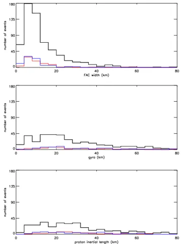
Figure 1 displays the number of events versus S(E), S(dn) and S(FAC) in the form of histograms, where black lines rep-resent monopolar events, red and blue lines reprep-resent con-verging and dicon-verging bipolar events, respectively. Each bin is 1 km wide. FAC width, proton gyroradius and proton in-ertial length are presented in the same form in Fig. 2. Note the extended range of the x-axis and that each bin in Fig. 2 is 4 km wide. Tables 1 and 2 give typical scale sizes, mean and median values, variance, skewness, 95th percentiles and the total number of events for the different types of electric fields. Mean and median values are given together with er-rors using the 95.5% confidence interval. “Typical” scale size or value refers to the most populated bin in Figs. 1 and 2. All spatial values are mapped to the ionosphere for reference. Skewness is a measure of the asymmetry of a distribution. All distributions in this study have positive skewness, i.e., the right tail (large scale sizes) is more pronounced than the left tail (small scale sizes). The higher the skewness, the more asymmetric the distribution.
It is seen in Tables 1 and 2, and in Figs. 1 and 2 that a majority of the events are monopolar and that there is an al-most equal amount of converging and diverging bipolar elec-tric field events. The S(E) distributions (top panel in Fig. 1) are similar for bipolar and monopolar events, and they have the same typical scale size (4–5 km). It can also be seen that the scale size distribution of the monopolar structures
Fig. 1. The number of events versus S(E), S(dn), and S(FAC), black lines represent monopolar events while red and blue lines rep-resent converging and diverging bipolar events, respectively.
is more asymmetric than the ones for bipolar structures. This is reflected in a higher median value and a larger skewness. There are more diverging than converging electric fields with scale sizes <4 km but otherwise no clear difference can be observed between these two types of bipolar electric fields.
The median scale sizes for the electric field, FAC and den-sity gradient are all in the range 4.2–4.9 km. This is true for both monopolar and bipolar events in all three parameters but the errors are larger for the bipolar events. The distributions of these scale sizes are also similar, and the number of events drops rather quickly as the scale size increases. For all three parameters, the drop is less steep for the monopolar events. This can be seen in a higher skewness for the monopolar events. The median values of S(E), S(FAC) and S(dn) are smaller for the diverging events compared to the converging events but generally, diverging and converging bipolar events have similar S(E), S(dn) and S(FAC) distributions.
The FAC widths have a median width of 9.7 km for monopolar electric fields and 8.3 (9.5) km for diverging (con-verging) bipolar electric fields, larger than the scale sizes of the electric field. (The uncertainty in FAC widths for diverg-ing events is large.) The distribution of the FAC widths (top
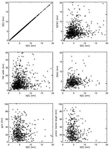
Fig. 2. The number of events versus FAC width, proton gyroradius and proton inertial length, black lines represent monopolar events while red and blue lines represent converging and diverging bipolar events, respectively. Note the increased range on the x-axis (com-pared to Fig. 1).
panel in Fig. 2) resembles the distributions in Fig. 1 but ex-tend into grater values. This shows that the electric field structures are embedded in the FAC regions. (Remember that S(FAC) is the full-width half-maximum of the current mag-nitude and FAC width is the the region with the same current direction.)
The proton gyroradius (middle panel in Fig. 2) and the pro-ton inertial length have also been calculated (bottom panel in Fig. 2). The populations from which these parameters are calculated are typically dominated by hot magnetospheric ions with a perpendicular temperature of a few keV.
The proton gyroradius has a different distribution, being larger than the previous scale sizes. The peak in the num-ber of monopolar events is broad, ranging from 4 km (similar to the typical values in S(E), S(FAC) and S(dn)) to 24 km. The median value is 22.3 km, so almost half of the events are associated with proton gyroradii outside of the broad peak region. The rather flat distribution is reflected in a low skew-ness. The bipolar events have median proton gyroradii of 25.7 km (diverging) and 23.4 km (converging).
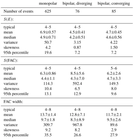
Fig. 3. Overview of all events in the form of scatter plots. The parameters plotted are S(E), S(FAC), FAC width, S(dn), proton gyroradii and proton inertial length, all vs. S(E). These values are mapped to the ionosphere.
The proton inertial lengths have a distribution similar to the gyroradius distribution. The median values are slightly greater while the typical proton inertial lengths for monopo-lar events overlap the range of typical gyroradii.
As was shown in Figs. 1 and 2, and in Tables 1 and 2, the typical, mean and median scale sizes of the electric field were similar to those of the FACs and density gradients. An-other way to describe the relation between the different pa-rameters is to present the data in the form of scatter plots. Figures 3 and 4 are such plots with the parameters plotted versus S(E). In Fig. 3, a general trend of increasing S(dn), S(FAC) and FAC width for increasing S(E) can be observed. The proton gyroradii and proton inertial length appear inde-pendent of S(E). The correlation coefficients are low, below 0.2 for all pairs. However, if the values instead are mapped to the equatorial plane, as done in Fig. 4, it is seen that also these two parameters correlate well with S(E). For S(dn), S(F AC) and FAC width, the correlation with S(E) is more clearly observed. The correlation coefficients between S(E) and the five other spatial scales, mapped to the equatorial plane, are for all pairs above 0.9 except for S(E) and proton
Fig. 4. Similar to Figure 3 but this time mapping to the equatorial plane.
gyroradius where the correlation coefficient is 0.8. (When the scale sizes are mapped to the ionosphere or to the equa-torial plane, the spread in latitude and altitude give different mapping factors for each event, hence the relationship be-tween the events in the two scatter plots can be different.) The improved correlation in the equatorial plane might indi-cate that the mechanism determining the scale sizes observed at Cluster’s altitude is located between the region of observa-tion and the equatorial plane.
3.2 Characteristics of S(E)
The influence of season and geomagnetic activity (as mea-sured by the Kp index) and possible dependence on MLT
and CGLat have been investigated. How S(E) is related to the electric field magnitude and the potential variation across the structure have also been considered.
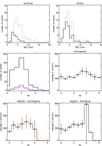
3.2.1 Influence of geomagnetic activity and season In the upper two panels in Fig. 5, the (monopolar and bipo-lar) events have been divided into four subsets. Events dur-ing summer and winter (periods of three months) have been
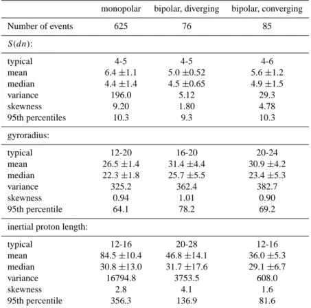
Table 1. Some statistical properties for the electric field scale size, S(E), and the field-aligned current scale size, S(FAC), and the FAC width. The results are separated for different types of electric fields. The values are mapped down to ionospheric altitude for reference and given in km. 11 events could neither be labelled monopolar nor bipolar by the routine used. For median and mean values, errors using the 95.5% confidence interval are given.
monopolar bipolar, diverging bipolar, converging
Number of events 625 76 85 S(E): typical 4–5 4–5 4–5 mean 6.9±0.57 4.5±0.41 4.7±0.45 median 4.9±0.71 4.2±0.51 4.6±0.56 variance 50.7 3.15 4.22 skewness 4.2 0.87 1.50 95th percentile 19.6 7.2 7.2 S(FAC): typical 4–5 4–5 5–6 mean 6.3±0.86 8.5±5.6 6.2±2.6 median 4.4±1.1 4.3±7.0 4.7±3.3 variance 114.3 592.4 149.5 skewness 10.4 6.5 8.0 95th percentile 13.1 12.9 9.6 FAC width: typical 4–8 4–8 4–8 mean 13.7±1.4 12.8±7.1 11.7±2.1 median 9.7±1.8 8.3±8.9 9.5±2.6 variance 309.7 967.8 89.6 skewness 9.2 8.2 2.9 95th percentile 35.5 26.6 27.9
separated after the level of geomagnetic activity under which they occur. The Kp index has been used to identify high
(Kp>3) and low (Kp≤3) activity events.
When comparing high activity events occurring during summer (solid line in the top left panel) with low activity events occurring during winter (dotted line in the top right panel), an increase in S(E) can be observed for the latter events. The typical scale size increases from 2–3 km to 4– 5 km and the distribution of events is also shifted towards greater S(E) for the low activity winter events compared to the high activity summer events. During the former times, both the background conductivity and the particle induced conductivity are lower than during the high activity summer events. This indicates that the ionospheric conductivity in-fluences the scale sizes of auroral structures as observed at high altitude in the form of intense electric fields. The typi-cal stypi-cale sizes are 3–4 km when Kp>3 during winter months
(solid line in the upper right panel) and 4–5 km when Kp≤3
during summer months (dotted line in the upper left panel). The mean and median values for the different subsets are given in Table 3 together with errors indicating the 95.5% confidence interval. The highest mean and median values
(6.9 and 5.1 km, respectively) are found for summer months during low activity while the lowest median value (3.6 km) is found for summer months during high activity and the lowest mean value (4.5 km) is found for winter months during high activity. There appear to be both a season and an activity de-pendence of which the latter is more important. The number of events in each of these four subsets are rather small. There are only 22 high Kpevents during summer, which gives some
uncertainty to the mean and median values for this subset. The middle and lower panels in Fig. 5 display the num-ber of events for bins in Kp and the average electric field
magnitude. The color coding is the same as in Fig. 1. Most events are found for medium activity (Kp=1–4) but
Johans-son et al. (2005) showed a weak increase in the probability of finding an event with increasing Kp. The average
elec-tric field magnitude (plotted together with error bars indicat-ing the 95.5% confidence interval) is found to increase with higher geomagnetic activity (except from the highest Kp
val-ues) consistent with the inverse relation between S(E) and the electric field magnitude (see below). The average electric field magnitudes of diverging (blue line) and converging (red line) bipolar and monopolar (black line) events are similar.
Table 2. Same kind of table as Table 1 but this time for the scale sizes of the density gradients, S(dn), and the proton gyroradii and the inertial proton scale. For median and mean values, errors using the 95.5% confidence interval are given.
monopolar bipolar, diverging bipolar, converging
Number of events 625 76 85 S(dn): typical 4-5 4-5 4-6 mean 6.4 ±1.1 5.0 ±0.52 5.6 ±1.2 median 4.4 ±1.4 4.5 ±0.65 4.9 ±1.5 variance 196.0 5.12 29.3 skewness 9.20 1.80 4.78 95th percentiles 10.3 9.3 10.3 gyroradius: typical 12-20 16-20 20-24 mean 26.5 ±1.4 31.4 ±4.4 30.9 ±4.2 median 22.3 ±1.8 25.7 ±5.5 23.4 ±5.3 variance 325.2 362.4 382.7 skewness 0.94 1.01 0.90 95th percentile 64.1 78.2 69.2
inertial proton length:
typical 12-16 20-28 12-16 mean 84.5 ±10.4 46.8 ±14.1 36.0 ±5.3 median 30.8 ±13.0 31.7 ±17.6 29.1 ±6.7 variance 16794.8 3753.5 608.0 skewness 2.8 4.1 1.6 95th percentile 356.3 136.9 81.6
Table 3. Mean and median scale sizes in km for the electric field, S(E), separated for summer and winter, and high (>3) and low (≤3) Kp. The values are mapped down to ionospheric altitude for reference and given in km. For median and mean values, errors using the 95.5% confidence interval are given.
summer, high Kp summer, low Kp winter, high Kp winter, low Kp
Number of events 22 82 49 92
mean 4.7±2.0 6.9±1.3 4.5±0.61 5.6±0.90
median 3.6±2.5 5.1±1.7 4.0±0.76 4.4±1.2
There are only two events in the bin for Kp6 and the error is
large, so the result in this bin is not reliable. 3.2.2 Potential and electric field magnitude
The potential variation across the electric field structure has been calculated for each event and is presented in the upper panels in Figs. 6 (monopolar events) and 7 (bipolar events), for bins in S(E). For S(E)>1 km, a weak increase in the potential with increasing S(E) is seen, from ∼0.9 kV to ∼2.9 kV for scale sizes of 9 km. This calculated potential is more reliable than the potential estimation made by Jo-hansson et al. (2005) and confirms the trend of an increasing potential with scale size, seen in that work. A peak in the
po-tential is found for S(E)=11 km and up to S(E)=14 km, with a maximum value of close to 6 kV. It is interesting that this scale size region corresponds to scale sizes of electric field structures observed in rocket measurements of arc associated electric fields (Marklund et al., 1982) and close to the typical arc widths observed by Knudsen et al. (2001).
For the bipolar events, a decrease in the potential varia-tion across the electric field structures is observed, contrary to what was seen for monopolar events. The converging and diverging events have maxima of 4.6 kV and 3.5 kV, re-spectively, before reaching rather constant values at approx-imately 2.0 kV and 1.4 kV, respectively. However, as was seen in Fig. 1, the number of events in the bipolar distribu-tions are rather few outside the peaks, raising uncertainties
Fig. 5. Upper panels: Number of events vs. S(E) for high (Kp>3, solid line) and low (Kp≤3, dotted line) geomagnetic activity and summer (left) and winter (right). Each season is defined as a three month period. Middle and lower panels: Number of events vs. Kp and average electric field magnitude for bins in Kp, events sepa-rated for monopolar (black line) and diverging (blue line) and con-verging (red line) bipolar electric fields. The error bars indicate the 95.5% confidence interval. If no error bar is indicated, then this bin contains no or only one event.
in the reliability of the results in the ends of the distributions. This can also be seen from the large error bars for most of the bins.
Figures 6 and 7 also display the distribution of events as a function of the electric field magnitude (bottom panels). The general trend is the same for monopolar and bipolar events. The typical magnitude is found to be close to 250 mV/m. For electric field magnitudes greater than 600 mV/m, the num-ber of events decreases rapidly. Rememnum-ber that the cutoff at 150 mV/m is due to the selection criterion when compiling the database.
The average electric field magnitude is plotted versus S(E) in the middle panels and is seen to be decreasing with increasing S(E) for both monopolar and bipolar events (ig-nore the last monopolar bin, with a large average electric field, since it contains only one event). This means that a
Fig. 6. Average potential V (upper panel) and average electric field magnitude (middle panel) for bins in S(E) together with number of events vs. electric field magnitude (bottom panel). Only monopolar events. All values mapped to the ionosphere. A selection criterion in this study was an electric field magnitude of at least 150 mV/m. The error bars indicate the 95.5% confidence interval.
smaller scale structure is likely to be more intense than a larger scale structure. Since the average potential across the monopolar structures increases with increasing scale size, the decrease in magnitude must be slower than the increase in scale size. This is only true for monopolar events. Among the bipolar electric fields, the converging ones are typically more intense than the diverging ones but the difference is small.
3.3 Related field-aligned currents
Lyons et al. (1979) observed a relation between the parallel current density and the parallel potential drop in the upward current region. The ratio Gup=jk/Vkis known as the
Lyons-Evans-Lundin constant. This can be compared with the theo-retically derived Knight relation (Knight, 1973) which in its linear regime can be written as jk=K18kwhere K is the
Knight conductance. The potentials, V⊥, determined from
integrations of the perpendicular electric fields in this study have been used together with the calculated field-aligned
Fig. 7. Same as Figure 6, but this time only converging (red) and diverging (blue) bipolar events. The error bars indicate the 95.5% confidence interval.
current, jz, to obtain a kind of proxy for the
Lyons-Evans-Lundin constant (assuming V⊥=Vk). Only one value is
cal-culated for each event. The results are found to be between 10−9−10−8S/m2, within the range of reported results of
the Lyons-Evans-Lundin constant, 10−10−10−8S/m2
(El-phic et al., 1998).
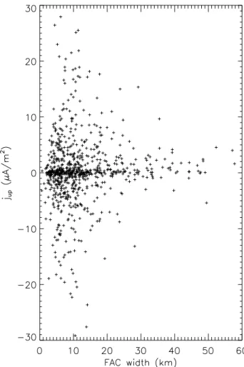
Figure 8 displays the FAC intensity as a function of FAC width, with values mapped to the ionosphere. Events where the intensity is small are found for all FAC widths. How-ever, the most intense FACs are associated with smaller FAC widths, and the number of intense FACs decreases with in-creasing FAC width. In this regard, the upward and down-ward FACs behave in the same way. This has also been ob-served by Peria et al. (2000). This characteristic is similar to the relation between the electric field magnitude and S(E). In both cases, an inverse proportionality to the spatial scale is observed. It is also worth noticing that the widths of up-ward and downup-ward FACs are similar.
Fig. 8. Scatter plot of the FAC magnitude vs. FAC width, both mapped to the ionosphere. Positive values are upward FAC.
4 Discussion
An important question in auroral physics is how to explain the discrepancies in scale sizes between, on one hand, re-ported optical observations, and on the other hand, theoret-ically predicted scales and in situ measurements, prevailing for both bright and black aurora. It is possible that the high-altitude structures, by some mechanism, are divided into sev-eral, narrower structures. This concept is illustrated by the re-sults in McFadden et al. (1999), although their smaller scales were an order of magnitude larger than the fine-scale auro-ral arcs. The work presented here focuses on the scale sizes of intense auroral electric fields observed by Cluster at high altitude (4–7 REgeocentric distance). Electric fields with
in-tensities (mapped to the ionosphere) less than 150 mV/m are not included. Based on earlier event studies (e.g., Johans-son et al., 2004) it is assumed that most of the events have a quasi-static structure.
The typical scale sizes of the studied intense electric fields (both monopolar and bipolar) are, when mapped to iono-spheric altitude, 4–5 km, with a median scale size of 4.8 km.
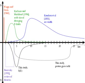
Fig. 9. A sketch summarizing some auroral scale size observations. The optical measurements of arc widths by Maggs and Davis (1968) and Knudsen et al. (2001) are shown in red and blue, respectively. The green line indicates the scale sizes for diverging bipolar electric fields observed by Freja (Karlsson and Marklund, 1996). A majority of the theories reviewed by Borovsky (1993) predicted scale sizes in the range 1–4 km; they are here represented by the purple rectan-gle. Results from this study are the solid black line, S(E), and the dashed-dotted black line, proton gyroradii.
This is somewhat larger than, but in rough agreement with, the theoretical predictions reviewed by Borovsky (1993). These are scale sizes in the gap of the arc width distribu-tion of the compiled studies by Maggs and Davis (1968) and Knudsen et al. (2001). The largest scale sizes in this study overlap with the small side tail of the meso-scale arcs widths in Knudsen et al. (2001). Figure 9 tries to summa-rize these different observations of auroral scales. The dis-tributions of the fine-scale and meso-scale auroral arcs ob-served by Maggs and Davis (1968) and Knudsen et al. (2001) (red and blue lines) are outlined. Typical electric field scale sizes observed by Cluster (this study, solid black line) and Freja (Karlsson and Marklund (1996), green line and diverg-ing electric fields only) fall into the gap between these two distributions. Karlsson and Marklund (1996) uses the same method (full-width half-maximum) to determine the scale sizes of the electric field structures as in this study. The me-dian scale size of the diverging electric fields observed in this study is 4.6 km, within the range of typical scale sizes (1– 5 km) observed by Freja. The electric fields investigated in this study are intense (≥150 mV/m at ionospheric altitude). Since an inverse relation between intensity and scale size has been found (see Fig. 6), lowering the limit in intensity for event selection would probably result in an increased number of larger scale sizes. Intense auroral electric field structures
have been shown to be related to plasma boundaries (Johans-son et al., 2006; Marklund et al., 2007), hence the scale sizes of electric field structures related to arc boundaries can be expected to be smaller than the arc widths determined by op-tical studies. The purple rectangle in Fig. 9 illustrates where most of the theories reviewed by Borovsky (1993) predict the arc widths to be found.
The widths or scale sizes of auroral arcs and structures re-ported in the literature are influenced by the resolution of the instrument used and how the data is presented. Stenbaek-Nielsen et al. (1998) mentioned, e.g., how the use of log-arithmic scales in particle energy and number flux plots can give too-wide scale sizes, compared to what is seen in optical observations. Using wide-angle lenses or narrow-field cam-eras can influence the scale size results of visible structures, and the choice will or will not give information of the large-scale context of the observation (Knudsen et al., 2001). The criterion used by Newell et al. (1996) selected events where the accelerated electron energy was 3–4 times larger than the source population thermal energy. This type of electron ac-celeration events, with a characteristic width of 28–35 km, was suggested to correspond to a cluster of individual arcs. The finest arc structures could not be resolved. The resolu-tion of the electric field measurements in this study is good enough to give confidence to the decrease in the S(E) distri-bution on the small scale side. The electric fields investigated are intense and therefore biased towards smaller scales (or so do the results indicate, see Fig. 6).
As discussed by Weimer et al. (1985), there is a critical scale size (proportional to the electron density and inversely proportional to the height-integrated Pedersen conductivity and the square root of the thermal energy), separating electric fields at high altitude that map down to the ionosphere and those that do not. Since it is the electric fields with scale sizes less than the critical value that do not map, implying parallel electric fields and particle acceleration, the electric fields in this study, which are small scale, are likely to not map down to the ionosphere. They should also correspond to auroral arcs. In earlier Cluster event studies of these kind of electric fields, the potential (calculated from the electric field) and the characteristic energy of up-going particles have been found to roughly agree (Johansson et al., 2004; Figueiredo et al., 2005), indicating non-mapping. For typical values of the in-put parameters, Weimer et al. (1985) give the critical scale sizes as 80 km, at ionospheric altitude. However, this criti-cal value will vary and might at times be smaller than 80 km. The shape of the auroral structures also influences how the electric field is mapped, or, equivalently, how the potential structures are closed. Spirals and folds have been shown to be associated with non-mapping electric fields, while sheet-like structures (stable arcs), were shown to partly extend down to the ionosphere (Hwang et al., 2006). Future studies consid-ering this subject are planned.
The distribution of the proton gyroradii for the events in this study is sketched as a dashed-dotted line in Fig. 9, clearly
separated from most other distributions. The proton gyro-radii distribution overlaps the arc widths reported by Knud-sen et al. (2001). The FAC and density gradient scale size distributions of this study are omitted since they are similar to the electric field scale size distribution.
Two parameters connected to Alfv´enic auroral activity are the electron inertial length, λe, and the Alfv´en wave resistive
scale, λA. Filamentary Alfv´enic field-aligned currents above
the aurora with widths similar to 2π λehave been observed by
FAST (Chaston et al., 2007). The electron inertial length has been calculated (and mapped to ionospheric altitude) for the events in this study. They were typically less then 0.75 km, so 2π λewould be ∼4.7 km. The widths of the currents
associ-ated with the intense electric fields of this study are typically larger, with median values of 8.3–9.7 km, for the different types of electric fields (see Table 1). The other parameter, λA, is typically of the order of 10 km (Pilipenko et al., 2004),
and well separated from the typical scale sizes of the intense electric fields investigated here.
The inverse relationship between electric field scale size and magnitude earlier reported from Freja (Karlsson and Marklund, 1996) and Cluster observations (Johansson et al., 2005), can be confirmed in this study. Also, a relationship between electric field scale size and the potential variation across the structure has been found. For the monopolar events, the potential tends to increase with increasing scale size, although the increase is weak. An inverse relationship between FAC width and FAC intensity has also been seen, consistent with earlier results on auroral FACs (Stasiewicz and Potemra, 1998). The FAC widths and intensities of up-ward and downup-ward currents were found to be similar. A symmetry in the thickness of the current sheets with respect to the polarity was also found by Peria et al. (2000) in a sta-tistical study of FACs derived from FAST data.
The ionospheric conductivity has been shown here to in-fluence the electric field scale size. During periods of high conductivity (summer months and high geomagnetic activity as measured by the Kp index), the scale sizes are typically
smaller. The dependence on geomagnetic activity is more significant. During periods of high activity, the electric field magnitudes are typically larger (as seen in Fig. 5). This is consistent with the inverse relation between scale size and electric field magnitude. In the downward FAC region, elec-trons are evacuated from the ionosphere, forming a plasma density hole, as has been shown in simulations (Karlsson and Marklund, 1998). Marklund et al. (2001) showed how a downward current region, to compensate for the depletion, widened so that the total current could remained roughly con-stant. During this time, the electric field scale size increased as well. This mechanism might explain why the electric field scale sizes in the downward current region are smaller for higher ionospheric conductivities. To maintain a certain cur-rent magnitude, a smaller region is required when the con-ductivity is higher. It is not understood why the same relation is seen for the electric field in the upward current region.
5 Conclusions
The main results of this study are:
1. The typical electric field, magnetic field and density gra-dient scale sizes are all 4–5 km (mapped to ionospheric altitudes), with no clear difference between scale sizes associated with monopolar, converging or diverging bipolar electric fields. However, the scale size distribu-tions for the monopolar events extend to greater values than the bipolar scale size distributions.
2. When mapped to the equatorial plane, S(dn), S(FAC), FAC width, proton gyroradius and proton inertial length correlate well with S(E).
3. The majority of the intense electric field structures (625 events) are monopolar, i.e., associated with S-shaped potential structures. Among the bipolar electric field signatures, associated with U-shaped potential struc-tures, there is approximately an equal number of con-verging and dicon-verging structures (85 and 76, respec-tively).
4. The electric field magnitude is inversely proportional to the scale size while the potential variation across monopolar structures has a small proportionality to the scale size.
5. The most intense field-aligned currents are found for small FAC widths. The widths of upward and down-ward FACs are similar.
6. Different ionospheric conductivity conditions are re-flected in different S(E), as high (low) conductivity fa-vors smaller (larger) scale sizes. Both seasonal varia-tions and geomagnetic activity influence S(E) but the latter is more important. Typical values are 2–3 km (4– 5 km) for Kp>3 (≤3) during summer (winter) months.
Acknowledgements. Work at the Royal Institute of Technology was
partially supported by the Swedish National Space Board and the Alfv´en Laboratory Centre for Space and Fusion Plasma Physics. S. Lil´eo acknowledges the support of the Fundac¸˜ao para a Ciˆencia e a Tecnologia (FCT) under the grant SFRH/BD/6211/2001.
Topical Editor I. A. Daglis thanks K. Lynch and another anony-mous referee for their help in evaluating this paper.
References
Andersson, L. and Ergun, R. E.: Acceleration of antiearthward elec-tron fluxes in the auroral region, J. Geophys. Res., 111, A07203, doi:10.1029/2005JA011261, 2006.
Balogh, A., Dunlop, M. W., Cowley, S. W. H., Southwood, D. J., Thomlinsson, J. G., Glassmeier, K. H., Musmann, G., L¨uhr, H., Buchert, S., Acuna, M., Fairfield, D., Slavin, J., Riedel, W., Schwingenschuh, K., and Kievelson, M.: The Cluster magnetic investigation, Space Sci. Rev., 79/1–2, 65–91, 1997.
Blixt, E. M. and Kosch, M. J.: Coordinated optical and FAST ob-servations of black aurora, Geophys. Res. Lett., 31, L06813, doi:10.1029/2003GL019 244, 2004.
Block, L. P.: Potential double layers in the ionosphere, Cosmic Electrodynamics, 3, 349–376, 1972.
Borovsky, J. E.: Auroral arc thickness as predicted by various theo-ries, J. Geophys. Res., 98, 6101–6138, 1993.
Chaston, C., Peticolas, L., Bonnell, J., Carlson, C., Ergun, R., Mc-Fadden, J., and Strangeway, R.: Width and brightness of auro-ral arcs driven by inertial Alfven waves, J. Geophys. Res., 108, 1091, doi:10.1029/2001JA007537, 2003.
Chaston, C., Hull, A., Bonnell, J., Carlson, C., Ergun, R., Strangeway, R., and McFadden, J.: Large parallel elec-tric fields, currents, and density cavities in dispersive Alfv´en waves above the aurora, J. Geophys. Res., 112, A05215, doi:10.1029/2006JA012007, 2007.
Chiu, Y. T. and Schulz, M.: Electrostatic model of a quiet auroral arc, J. Geophys. Res., 83, 629–642, 1978.
Elphic, R. C., Bonnell, J., Strangeway, R., Kepko, L., Ergun, R., McFadden, J., Carlson, C., Peria, W., Cattell, C., Klumper, D., Shelley, E., Peterson, W., Moebius, E., Kistler, L., and Pfaff, P.: The auroral current circuit and field-aligned currents observed by FAST, Geophys. Res. Lett., 25, 2033–2036, 1998.
Figueiredo, S., Marklund, G., Karlsson, T., Johansson, T., Ebihara, Y., Ejiri, M., Ivchenko, N., Lindqvist, P.-A., Nilsson, H., and Fazakerley, A.: Temporal and spatial evolution of discrete auro-ral arcs as seen by Cluster, Ann. Geophys., 23, 2531–2557, 2005, http://www.ann-geophys.net/23/2531/2005/.
Galperin, Y. I.: Multiple scales in auroral plasmas, J. Atmos. Sol.-Terr. Phy., 64, 211–229, 2002.
Gustafsson, G., Bostr¨om, R., Holback, B., Holmgren, G., Lund-gren, A., Stasiewicz, K., ˚Ahl´en, L., Mozer, F., Pankow, D., Har-vey, P., Berg, P., Ulrich, R., Pedersen, A., Schmidt, R., Butler, A., Fransen, A., Klinge, D., Thomsen, M., F¨althammar, C.-G., Lindqvist, P.-A., Christenson, S., Holtet, J., Lybekk, B., Stein, T., Tanskanen, P., Lappalainen, K., and Wygant, J.: The Electric Field and Wave Experiment for the Cluster mission, Space Sci. Rev., 79/1–2, 137–156, 1997.
Hudson, M. K. and Mozer, F. S.: Electrostatic shocks, double lay-ers, and anomalous resistivity in the magnetosphere, Geophys. Res. Lett., 5, 131–134, 1978.
Hwang, K.-J., Lynch, K. A., Carlson, C. W., Bonell, J. W., and Peria, W. J.: Fast Auroral Snapshot observations of perpendicular DC electric field structures in downward cur-rent regions: Implications, J. Geophys. Res., 111, A09206, doi:10.1029/2005JA011472, 2006.
Jasperse, J. R.: Ion heating, electron acceleration, and the self-consistent E-field in downward auroral current regions, Geophys. Res. Lett., 25, 3485–3488, 1998.
Jasperse, J. R. and Grossbard, N. J.: The Alfv´en-F¨althammar formula for the parallel E-field and its analogue in downward auroral-current regions, IEEE T. Plasma Sci., 28, 1874–1886, 2000.
Johansson, T., Figueiredo, S., Karlsson, T., Marklund, G., Fazak-erley, A., Buchert, S., Lindqvist, P.-A., and Nilsson, H.: Intense high-altitude auroral electric fields - temporal and spatial charac-teristics, Ann. Geophys., 22, 2485–2495, 2004,
http://www.ann-geophys.net/22/2485/2004/.
Johansson, T., Karlsson, T., Marklund, G., Figueiredo, S.,
Lindqvist, P.-A., and Buchert, S.: A statistical study of intense electric fields at 4–7 RE geocentric distance using Cluster, Ann. Geophys., 23, 2579–2588, 2005,
http://www.ann-geophys.net/23/2579/2005/.
Johansson, T., Marklund, G., Karlsson, T., Lil´eo, S., Lindqvist, P.-A., Marchaudon, P.-A., Nilsson, H., and Fazakerley, A.: On the profile of intense high-altitude auroral electric fields at magneto-spheric boundaries, Ann. Geophys., 24, 1713–1723, 2006, http://www.ann-geophys.net/24/1713/2006/.
Karlsson, T. and Marklund, G.: A statistically study of intense low-altitude electric fields observed by Freja, Geophys. Res. Lett., 23, 1005–1008, 1996.
Karlsson, T. and Marklund, G.: Simulations of effects of small-scale auroral current closure in the return current region, Physics of Space Plasmas, 15, 401–406, 1998.
Keiling, A., Wygant, J. R., Cattell, C. A., Mozer, F. S., and Russell, C. T.: The Global Morphology of Wave Poynting Flux: Powering the Aurora, Science, 299, 383–386, 2003.
Kimball, J. and Hallinan, T.: A morphological study of black vortex streets, J. Geophys. Res., 103, 14 683–14 695, 1998.
Knight, S.: Parallel electric field, Planet. Space Sci., 21, 741–750, 1973.
Knudsen, D. J., Donovan, E. F., Cogger, L. L., Jackel, B., and Shaw, W. D.: Width and structure of mesoscale optical auroral arcs, Geophys. Res. Lett., 28, 705–708, 2001.
Lyons, L., Evans, D., and Lundin, R.: An observed relation between magnetic field aligned electric fields and downward electron en-ergy fluxes in the vicinity of auroral forms, J. Geophys. Res., 84, 457–461, 1979.
Maggs, J. E. and Davis, T. N.: Measurements of the thickness of auroral structures, Planet. Space Sci., 216, 205–209, 1968. Marklund, G., Sandahl, I., and Opgenoorth, H.: A study of the
dy-namics of a discrete auroral arc, Planet. Space Sci., 30, 179–197, 1982.
Marklund, G., Karlsson, T., and Clemmons, J.: On low-altitude par-ticle acceleration and intense electric fields and their relation to black aurora, J. Geophys. Res., 102, 17 509–17 522, 1997. Marklund, G., Ivchenko, N., Karlsson, T., Fazakerley, A., Dunlop,
M., Lindquist, P.-A., Buchert, S., Owen, C., Taylor, M., Vaivalds, A., Carter, P., Andr´e, M., and Balogh, A.: Temporal evolution of the electric field accelerating electrons away from the auroral ionosphere, Nature, 414, 724–727, 2001.
Marklund, G., Johansson, T., Lil´eo, S., and Karlsson, T.: Cluster observations of an auroral potential and associated field-aligned current reconfiguration during thinning of the plasma sheet boundary layer, J. Geophys. Res., 112, A01208, doi:10.1029/2006JA011804, 2007.
McFadden, J. P., Carlson, C. W., and Ergun, R. E.: Microstructures of the auroral acceleration region as observed by FAST, J. Geo-phys. Res., 104, 14 453–14 480, 1999.
Mozer, F. S.: Electric field mapping in the ionosphere at the equa-torial plane, Planet. Space Sci., 18, 259–263, 1970.
Newell, P. T., Lyons, K. M., and Meng, C.-I.: A large survey of electron acceleration events, J. Geophys. Res., 101, 2599–2614, 1996.
Peria, W., Carlson, C., Ergun, R., McFadden, J., Bonnell, J., Elphic, R., and Strangeway, R.: Characteristics of field-aligned currents near the auroral acceleration region: FAST observations, in Mag-netospheric Current Systems, Geophys. Monogr. Ser., 118, 181–
189, 2000.
Peticolas, L. M., Hallinan, T. J., Stenbeck-Nielsen, H. C., Bonnell, J. W., and Carlson, C. W.: A study of black aurora from aircraft-based optical observations and plasma measurements on FAST, J. Geophys. Res., 107, 1217, doi:10.1029/2001JA900157, 2002. Pilipenko, V., Fedorov, E., Engebretson, M., and Yumoto, K.: Energy budget of Alfven wave interactions with the au-roral acceleration region, J. Geophys. Res., 109, A10204, doi:10.1029/2004JA010440, 2004.
R`eme, H., Bosqued, J. M., Sauvaud, J. A., Cros, A., Dandouras, J., Aoustin, C., Bouyssou, J., Camus, T., Cuvilo, J., Martz, C., M´edale, J. L., Perrier, H., Romefort, D., Rouzaud, J., D’Uston, C., M¨obius, E., Crocker, K., Granoff, M., Kistler, L. M., Popecki, M., Hovestadt, D., Klecker, B., Paschmann, G., Scholer, M., Carlson, C. W., Curtis, D. W., Lin, R. P., Mcfadden, J. P., Formisano, V., Amata, E., Bavassano-Cattaneo, M. B., Baldetti, P., Belluci, G., Bruno, R., Chionchio, G., Lellis, A. D., Shel-ley, E. G., Ghielmetti, A. G., Lennartsson, W., Korth, A., Rosen-bauer, H., Lundin, R., Olsen, S., Parks, G. K., Mccarthy, M., and Balsiger, H.: The Cluster ion spectrometry (CIS) experiment, Space Sci. Rev., 19/1–2, 303–350, 1997.
Song, Y. and Lysak, R. L.: The physics in the auroral dynamo re-gions and auroral particle acceleration, Phys. Chem. Earth (C), 26, 33–42, doi:10.1016/S1464–1917(00)00087–8, 2001. Stasiewicz, K. and Potemra, T.: Multiscale current structures
ob-seved by Freja, J. Geophys. Res., 103, 4315–4325, 1998.
Stenbaek-Nielsen, H. C., Hallinan, T. J., Osborne, D. L., Kimball, J., Chaston, C., McFadden, J., Delory, G., Temerin, M., and Carl-son, C.: Aircraft observations conjugate to FAST: Auroral arc thickness, Geophys. Res. Lett., 25, 2073–2076, 1998.
Temerin, M. and Carlson, C.: Current-Voltage relations in the downward auroral current region, Geophys. Res. Lett., 25, 2365– 2368, 1998.
Temerin, M., Cerny, K., Lotko, W., and Mozer, F.: Observations of double layers and solitary waves in the auroral plasma, Phys. Rev. Lett., 48, 1175–1179, 1982.
Trondsen, T. S. and Cogger, L.: High-resolution television observa-tions of black aurora, J. Geophys. Res., 102, 363–378, 1997. Vaivads, A., Andre, M., Buchert, S., Eriksson, A., Olsson, A.,
Wahlund, J.-E., Janhunen, P., Marklund, G., Kistler, L., Mouikis, C., Winningham, D., Fazakerley, A., and Newell, P.: Discrete au-roral arc, electroststic shock and suprathermal electrons powered by dispersive, anomalously resistive field line resonance, Geo-phys. Res. Lett., 30, 1106, doi:10.1029/2002GL016006, 2003. Weimer, D. R. and Gurnett, D. A.: Large-Amplitude Auroral
elec-tric Fields Measured With DE 1, J. Geophys. Res., 98, 13 557– 13 564, 1993.
Weimer, D. R., Goertz, C. K., Gurnett, D. A., Maynard, N. C., and Burch, J. L.: Auroral zone electric fields from DE 1 and DE 2 at magnetic conjunctions, J. Geophys. Res., 90, 7479–7494, 1985.