Suitability of quantum cascade laser spectrometry for CH<sub>4</sub> and N<sub>2</sub>O eddy covariance measurements

(1)

HAL Id: hal-00297884

https://hal.archives-ouvertes.fr/hal-00297884

Submitted on 12 Apr 2007

HAL is a multi-disciplinary open access

archive for the deposit and dissemination of sci-entific research documents, whether they are pub-lished or not. The documents may come from teaching and research institutions in France or abroad, or from public or private research centers.

L’archive ouverte pluridisciplinaire HAL, est destinée au dépôt et à la diffusion de documents scientifiques de niveau recherche, publiés ou non, émanant des établissements d’enseignement et de recherche français ou étrangers, des laboratoires publics ou privés.

Suitability of quantum cascade laser spectrometry for

CH4 and N2O eddy covariance measurements

P. S. Kroon, A. Hensen, H. J. J. Jonker, M. S. Zahniser, W. H. van ’T Veen,

A. T. Vermeulen

To cite this version:

P. S. Kroon, A. Hensen, H. J. J. Jonker, M. S. Zahniser, W. H. van ’T Veen, et al.. Suitability of quantum cascade laser spectrometry for CH4 and N2O eddy covariance measurements. Biogeosciences Discussions, European Geosciences Union, 2007, 4 (2), pp.1137-1165. �hal-00297884�

(2)

BGD

4, 1137–1165, 2007 Suitability QCL for eddy covariance P. S. Kroon et al. Title Page Abstract Introduction Conclusions References Tables Figures ◭ ◮ ◭ ◮ Back Close

Full Screen / Esc

Printer-friendly Version Interactive Discussion

EGU Biogeosciences Discuss., 4, 1137–1165, 2007

www.biogeosciences-discuss.net/4/1137/2007/ © Author(s) 2007. This work is licensed

under a Creative Commons License.

Biogeosciences Discussions

Biogeosciences Discussions is the access reviewed discussion forum of Biogeosciences

Suitability of quantum cascade laser

spectrometry for CH

₄

and N

₂

O eddy

covariance measurements

P. S. Kroon1, A. Hensen1, H. J. J. Jonker2, M. S. Zahniser3, W. H. van ’t Veen1, and A. T. Vermeulen1

1

Energy research Centre of the Netherlands (ECN), Department of Air Quality and Climate Change, Netherlands

2

TU Delft, Department of Multi-Scale Physics, Research group Clouds, Climate and Air Quality, Netherlands

3

Aerodyne Research, Inc., USA

Received: 20 March 2007 – Accepted: 3 April 2007 – Published: 12 April 2007 Correspondence to: P. S. Kroon (p.kroon@ecn.nl)

(3)

BGD

Full Screen / Esc

EGU

Abstract

A quantum cascade laser spectrometer was evaluated for eddy covariance measure-ments of CH4 and N2O using laboratory tests and three months of continuous

mea-surements. Moreover, an indication was given of CH₄ and N₂O exchange. All four required criteria for eddy covariance measurements related to continuity, sampling

5

frequency, precision and stationarity were checked. The system had been running continuously at a dairy farm on peat grassland in the Netherlands from 17 August to 6 November 2006. An automatic liquid nitrogen filling system was employed for unattended operation of the system. A sampling frequency of 10 Hz was obtained using a 1 GHz PC system. A precision of 2.6 and 0.3 ppb Hz−1/2 was obtained for

10

CH4 and N2O, respectively. However, it proved to be important to calibrate the

equipment frequently using a low and a high standard. Drift in the system was re-moved using a 120 s running mean filter. Average fluxes and standard deviations in the averages of 484±375 ngC m−2s−1(2.32±1.80 mg m−2h−1) and 39±62 ngN m−2s−1 (0.22±0.35 mg m−2h−1) were observed. About 40% of the total N₂O emission was due

15

to a fertilizing event.

1 Introduction

The greenhouse gasses Methane (CH₄) and Nitrous oxide (N₂O) play a major role in global warming with global warming potentials 21 and 310 times greater than CO2,

respectively (IPCC,2001). Agricultural soils are major sources of both gasses (IPCC,

20

2006). However, there are significant uncertainties in the estimated CH₄ and N₂O fluxes, mainly owing to a combination of complexity of the source (i.e. spatial and tem-poral variation), limitations in the measurement equipment and the methodology used to obtain the emissions. High-frequency micrometeorological methods are often used to obtain integrated emission estimates on a hectare scale that also have continuous

25

(4)

BGD

Full Screen / Esc

EGU the requirements for eddy covariance (EC) operation. For example, a limited number

of eddy correlation measurements have been published using lead salt tunable diode laser spectrometers (TDL), but these often suffer from drift and insensitivity effects (e.g. Smith et al.,1994;Wienhold et al.,1994;Laville et al.,1999;Hargreaves et al., 2001;Werle and Kormann,2001).

5

Quantum cascade laser spectrometers (QCL) are more stable and sensitive instru-ments compared to TDL-systems. QCL spectroscopy was first demonstrated in 1994 (Faist et al.,1994). Detailed descriptions of the working principles of QCL are given in Nelson et al.(2002) andJim ´enez et al.(2005). Nelson et al.(2004) pointed out that the instrument must satisfy four criteria for performing CH₄ and N₂O EC-measurements.

10

First, a precision of about 4 ppb and 0.3 ppb is required for CH₄ and N₂O at average ambient concentrations of 1800 ppb and 320 ppb, respectively. Second, the drift should be minimal during a period of atmospheric stationarity on the order of 30 min. Third, the measurement frequency should be in the order of 10 Hz (Monteith and Unsworth, 1990) to evaluate the small eddies as well. Finally, the instrument should operate on

15

a continuous basis. Nelson et al. (2004) showed that quantum cascade lasers can meet these criteria. However, this conclusion is mainly based on technical and theoret-ical considerations. Therefore, it is desirable to perform practtheoret-ical tests to validate the suitability of a QCL for EC-measurements.

This paper discusses the performance of the QCL for EC-measurements using

lab-20

oratory tests and three months of continuous measurements at a dairy farm on peat grasslands in the Netherlands. Moreover, an indication will be given of CH4 and N2O

emissions behaviour during these months. A description of the experimental site and the climatic conditions is given in Sect.2. Section3is devoted to the instrumentation and the methodology. The results are shown in Sect.4. Finally, the conclusions and

25

(5)

BGD

Full Screen / Esc

EGU

2 Experimental site and climatic conditions

The measurements were performed at an intensively managed dairy farm. This farm is located at Oukoop near the town of Reeuwijk in the Netherlands (Coord N 52◦01′15′′, E 4◦01′17′′). The surrounding area of the measurement location has soil consisting of a clayey peat or peaty clay layer of up to 25 cm on up to 12 m eutrophic peat deposits.

5

Rye grass (Lolium perenne) is the most dominate grass species with rough bluegrass (Poa trivialis) often co-dominant. Clover species constitute less than 1% of the veg-etation (Veenendaal et al., 20071). About 21% of the area is open water (Nol et al., 20072). The mean elevation of the polder is between 1.6 and 1.8 m below sea level. Ditch water level in the polder is being kept at –2.39 in winter and –2.31 m in summer

10

(Veenendaal et al., 20071). The climate is temperate and wet, with an average temper-ature of 10.3◦C in 2004 and 2005, and with an average annual precipitation of about 870 mm in 2004 and 2005. The dominating wind direction is southwest (Veenendaal et al., 20071). A summary of the main characteristics is given in Table1.

Manure and fertilizing are applied from February to September. Manure

15

and artificial fertilizing application were about 55 m3ha−1yr−1 (253 kgN ha−1yr−1) and 320 kg ha−1yr−1 (84 kgN ha−1yr−1) in 2006. Continuous CH4 and N2O

EC-measurements (coverage of 87%) had been performed from August 17th to 6 Novem-ber 2006. The averaged temperature over the measurement period was 17◦C and 55 kgN ha−1 cow manure was applied on 14 September 2006.

20

1

Veenendaal, E. M., Kolle, O., Leffelaar, P., et al.: Land use dependent CO2exchange and

carbon balance in two grassland sites on eutropic drained peat soils, Biogeosci. Discuss., submitted, 2007.

2

Nol, L., Verburg, P. H., Heuvelink, G. B. M., and Molenaar, K.: Effect of land cover data on N₂O inventory in fen meadows, J. Environ. Quality, submitted, 2007.

(6)

BGD

Full Screen / Esc

EGU

3 Instrumentation and methodology

The four required criteria for performing EC-measurements of CH4 and N2O were

val-idated using laboratory tests and three months of field measurements. The laboratory tests consisted of concentration measurements to evaluate precision, stationary and sampling frequency. The field measurements consisted of three months of

continu-5

ous EC-measurements with which the continuity of the system was checked and a first indication of the CH₄and N₂O exchange was obtained.

3.1 Instrumentation

The QCL was placed in a container of 2×2×2 m at about 20 m east from the mast. The measurement height was 3m and the mast was positioned in the middle of the

10

field. Terrain around the towers was flat and free of obstruction for at least 600 m in all directions, except for the container. Wind speed, air temperature, CH4 and N2O

concentrations were measured with a system consisting of a three-dimensional sonic anemometer (model R3, Gill Instruments, Lymington, UK) and a quantum cascade laser spectrometer (model QCL-TILDAS-76, Aerodyne Research Inc., Billerica MA,

15

USA).

The QCL has a multi-pass cell with an optical path of 76 m and a volume of 0.5 l maintained between 15 and 40 Torr. The QCL has two laser positions available that can be used simultaneously. During these experiments only one laser was used which operated at the 1270 and 1271 cm−1 absorption lines for CH₄ and N₂O, respectively.

20

The laser was used in pulsed mode. A sequence of laser light pulses, each with dura-tion of about 10 ns, is divided by a beam splitter and sent through the multi-pass cell and along a bypass. Both beams are detected on a single detector sequentially with the bypass pulse arriving 250 ns before the multi-pass pulse. The laser frequency is tuned through the absorption lines using a sub-threshold current applied to laser

be-25

tween pulses. The laser light intensity is lower at the start of the pulse sequence at about 1269 cm−1 and increases towards the end of the pulse sequence at 1272 cm−1.

(7)

BGD

Full Screen / Esc

EGU This is true for both beams. The bypass signal is used to normalise the signal obtained

from the multi-pass cell. The result is a pattern that shows a relatively constant inten-sity ratio with a decrease in light inteninten-sity passing through the multi-pass cell at the frequencies of the two absorption lines.

The QCL-software uses spectral parameters listed in the HITRAN database to make

5

a fit to this pattern and derive approximate CH4and N2O gas concentrations (Rothman

and Barbe, 2003). With pulsed-QCLs, the laser line width is on the same order as the Voigt line width of the absorber, and therefore must be considered in the fitting routine by convolving the laser line shape with the molecular absorbance. The non-Gaussian shape of the laser line profile can result in underestimating the molecular

10

concentration from 10 to 20% depending on the line depth. Calibration with known standards is therefore necessary for greater accuracy. A more detailed description of the QCL is found inNelson et al.(2002) andJim ´enez et al.(2005).

The detectors of the QCL spectrometer require cooling by liquid nitrogen for maxi-mum sensitivity in the wavelength region. The 0.5 l dewar on the optical table needs

15

to be refilled approximately every 24 h. An automated filling unit was used (with a 50 l storage dewar produced by Norhoff, Netherlands). With this setup visits to the instru-ment were necessary only once a week. In order to minimize drift owing to changing alignment the temperature cover and optical table were maintained at 35±0.1◦C by thin film heaters. The laser electronics were stabilized at±0.1◦C using circulating

wa-20

ter bathNelson et al.(2004). Otherwise, a variation in reported mixing ratios can occur when ambient temperature surpasses the system temperature as large as 2 ppb◦C−1 for N₂O (Nelson et al.,2004).

The air inlet was located at the sonic height of 3 m above the field. A 25 m PTFE inlet tube with a diameter of 0.25 inch was used. At the QCL inlet a 0.01 µm filter (DFU

25

filter tube grade BQ, Balston, USA) was used to avoid degradation of the multi-pass cell mirrors. The flow and cell pressure were controlled with a needle valve at the inlet of the multi-pass cell. A vacuum pump (TriScoll 600, Varian Inc, USA) with a maximum volume flow rate of 400 l min−1was located downstream of the multi-pass cell. The QCL

(8)

BGD

Full Screen / Esc

EGU was calibrated at least once a week using mixtures in N₂/O₂of 1700 and 5100 ppb for

CH4and 300 and 610 ppb for N2O (Scott speciality gasses, Netherlands)

The sonic anemometer data and the QCL-output were logged using the RS232 out-put and processed using a data acquisition program developed at ECN, following the procedures of McMillen (1988). Both the QCL and the eddy covariance computer

5

were available for remote control. The sampling frequency of the QCL was not ex-actly uniform. The average time between two samples was about 0.11 s. The sonic anemometer produced an uniform sampling rate of 20.88 Hz. The data acquisition pro-gram saved both the QCL and sonic data in the same file at 20.88 Hz using the last measured concentration value. As a consequence, the contribution to CH₄ and N₂O

10

fluxes of large eddies, with sampling frequencies below 5 Hz, were sampled well, but the contribution of smaller eddies were not.

3.2 Methods

The net ecosystem exchange (NEE) of both gasses is given by Zh 0 S_cd z | {z } NEE = Zh 0 ∂c ∂td z | {z } Storage + w′_c′_| h | {z } Eddy flux (1) 15

when horizontal homogeneity, stationarity and a flat terrain are assumed. The NEE consists of the sources, sinks and surface flux (e.g. based onHoogendoorn and van der Meer,1991andNieuwstadt,1998).

Evaluation of the eddy flux consisted of different phases. First, the raw data of w(t)

andc(t) was analyzed by eye on spikes and malfunctioning. Then, all concentration

20

data was corrected using a two-point calibration factor based on weekly calibrations. The standards were 1700 and 5100 ppb for CH₄, and 300 and 610 ppb for N₂O (Scott speciality gasses, Netherlands). The two-point calibration factorfLHis defined by

fLH=

SH− SL

MH− ML

(9)

BGD

Full Screen / Esc

EGU in whichSLandSHare the low and high standard values in ppb andMLandMHare the

low and high measured values in ppb. The corrected concentration was found using this factor and the following equation

Ccor= fLHCuncor (3)

withCuncor the uncorrected concentration value in ppb andCcorthe corrected

concen-5

tration value in ppb. It was important to correct the data using this factor seeing that the QCL does not provide absolute values for the mixing ratios. Next, the time averaging, which was based on a running mean, and mean removal operations were performed by ˜ wk= (1 − ∆t_τ f ) ˜w_k−1+∆t_τ f wk (4) 10 ˜ ck= (1 − ∆t_τ f ) ˜c_k−1+∆t_τ f ck (5) w′_c′₌ 1 ns ns X k=1 (wk− ˜wk)(ck− ˜ck). (6)

where k is the sampling number, ∆t is the interval between two samples in s, τf is the

running mean filter time constant and ns is the amount of samples in the averaging

period (Lee et al.,2004). The fluxes F_c were calculated using a 120 s running mean

15

filter time constant and a 30-min averaging time. Furthermore, the time lag between the sonic anemometer and QCL-data caused by the length of the sampling tube was determined using the covariance as function of delay time, which is given by

F_c= covwc(n∆t) = wk′c ′ k+n∆t = 1 n_s n_s X k=1 w_k′c′_k+n∆t (7)

where the delay time is defined by n∆t in which n denotes the amount of time steps.

20

(10)

BGD

Full Screen / Esc

EGU exact delay time. The exact delay time is dependent on the flow rate in the tube. The

flow rate itself is dependent on the resistance of the system, which is mainly dependent on the conditions of the inlet filter. If the inlet filter becomes dirty, the flow rate will decrease. The gradual increase of the resistance of the inlet filter resulted in a slow decrease of the mass flow rate. In our case, the mass flow rates decreased from 22 to 8

5

standard l min−1and in consequence the delay time increased from 1.5 to 7.6 s. These changes were monitored using the cell pressure. However, the exact delay times were calculated for each day by determining the maximum in covariance of the fluxes.

The Reynolds number for the inlet configuration ranged from about 5020 to 1720 at the high and low flow, respectively. Mixing of air in the inlet tube led to a decreased

10

contribution of the higher frequencies (i.e. the small eddies) to the calculated flux. Ac-cording toLenschow and Mann(1994) the damping effect was estimated to be smaller than 50% for frequencies below 3 Hz when cell pressures were above 35 Torr. A thor-ough investigation on the damping effect could be done using an empirical correction approach given byAmmann et al. (2006). This correction approach is based on the

15

flux ogives which are defined by

Og_wc(fm) = m X i=1 |Cowc(fi)| fi= i (ns− 1)∆t ; m = 1, 2, ...,h(ns− 1)∆t 2∆t i (8)

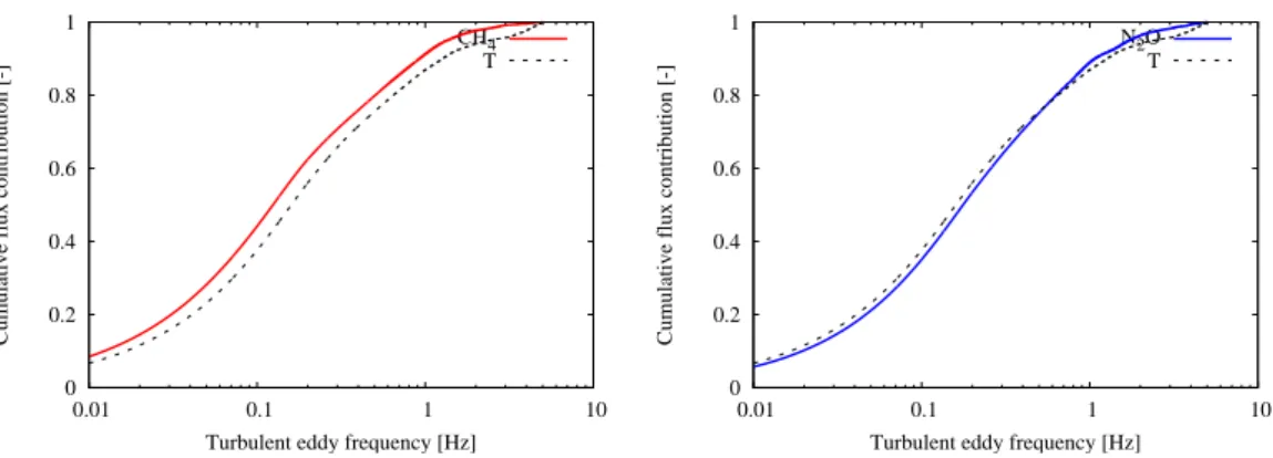
wheref represents frequency in Hz and Cowc the co-spectrum. Figure 1 shows the

normalized ogives of the CH4, N2O and sensible heat flux belonging to 7 October 2006

20

between 12:00–14:00, which was a neutral period with mean wind velocity of about 7 ms−1. These ogives were determined using block averaging and an averaging time of 30 min. It can be seen that damping effects were almost negligible for this period. Nevertheless, more analyses should be done to investigate the effect of damping on the flux values for all circumstances.

(11)

BGD

Full Screen / Esc

EGU The storage term was calculated using the QCL data according to Eq. (1). The

calibration-corrected NEE was given by adding the storage and the eddy flux term. The NEE data were flagged using the instationarity test ofFoken and Wichura(1996). Finally, the fetch was checked by a footprint model based on the Kormann-Meixner method (Neftel et al., 20073; Kormann and Meixner, 2001). The 30-min NEE value

5

was rejected when less than 70% of the flux came from the dairy farm site.

4 Results

4.1 Performance EC-measurements

As described byNelson et al.(2004), an EC-measurement system should satisfy four criteria related to continuity, sampling frequency, precision and stationarity. As for

con-10

tinuity, the system proved to be very stable as far as alignment and laser drift was con-cerned. The most sensitive part of the system proved to be the liquid nitrogen refilling unit. In summer with high temperatures the container became too hot inside which led to changing alignment. An extra ventilator was installed on the container which proved to be sufficient to keep the temperature inside the container below 35◦C. Continuous

15

CH4 and N2O EC-measurements (total data coverage 87%) had been obtained from

17 August to 6 November 2006 with about one visit per week excluding the intensive campaigns.

For most conditions a sampling frequency of about 10 Hz is sufficient to perform EC-measurements (Ammann,1998). According toNelson et al.(2004) this necessitates

20

both a fast electronic signal processing time and a rapid sampling cell response time. The signal processing time is dependent on the complexity of the spectrum and the number of spectral lines included in the fit. Laboratory tests, using the Aerodyne TDL-Wintel software running on a 1 GHz PC showed that 20 Hz acquisition was possible

3

Neftel, A., Spirig, C., and Ammann C.: A simple tool for operational footprint evaluations, Environ. Pollut., submitted, 2007.

(12)

BGD

Full Screen / Esc

EGU for 2 or 3 gas species simultaneously. However, the overall frequency response of the

system is limited by sampling cell response time rather than the signal processing time. A sampling cell response time (1/e) of τ=0.07 s was obtained using the 400 l min−1

Varian Vacuum pump with a cell volume of 0.5 l. This gives an effective bandwidth limitation of 1/(2πτ)∼3 Hz which is slightly less than the Nyquist frequency of 5 Hz using

5

a sampling rate of 10 Hz. So, the flux could be underestimated due to to missing contributions of the small eddies by damping effects (see Sect.3.1, non exactly uniform sampling (see Sect.3.1) and limited response time.

The system precision and stationarity are strongly dependent on the drift of the in-strument. An indication of both properties can be given using an Allan variance

anal-10

ysis (e.g.Allan,1966; Werle and Slemr, 1991). In this method, the variances in the time series of reported mixing ratio when sampling a constant source from a calibra-tion take are plotted as a funccalibra-tion of integracalibra-tion time. The Allan variance decreases witht−1 when random noise dominates. This decrease continues to a point at which drift effects start to influence the measurements. Due to instrument drift at longer times

15

the Allan variance increases again. The minimum is indicated byτAandσA, which

rep-resent the stability time in s and the sensitivity in ppb belonging to this stability time. Apart from this, the y-axis intersection point gives an indication of short term precision of the system using

σ = σ1sf

−1/2

s (9)

20

in whichfs is the sampling frequency in Hz. Precision and stationarity are determined

by drift effects which depend on the instrumental configuration. The most important factor to minimize drift is proper thermal control of optics and the electronics to main-tain constant dimensionality and a stable electrical environment of the system. Preci-sion may also be improved by optimizing the least-squares fitting routines to minimize

25

residuals between data and fit, and by optimizing the optical alignment of the system. Optical inference fringes, which can lead to instabilities with continuous wave laser systems, are not as important in pulsed laser systems. However, since the pulsed

(13)

BGD

Full Screen / Esc

EGU laser is operated near threshold to maintain a narrow laser width, the short term

pre-cision is generally limited by detector noise. The influence of alignment and therefore the amount of laser power on the detector was investigated using laboratory tests. It was found that the sensitivity was doubled when power at the detector was doubled by alignment optimization. A summary of short term performance for a typical range of

5

operating conditions is given in Table2.

The minimum in the Allan variance defining the long-term stability which can be reached using this instrument is now about 200 s (Nelson et al.,2004). These results are in agreement with Werle and Slemr (1991) andWysocki et al. (2005). However, CH4and N2O fluxes are often calculated over an averaging time of 30 min. The choice

10

of this interval is mainly based on the measurement height and the stability of the atmo-sphere since the size of the contributing eddies depends on those properties. Larger eddies contribute when the measurement height becomes higher and the atmospheric circumstances are more unstable. An overestimation of flux is possibly caused by instrumental drift effects on time scales from 200 s to the longest averaging time of

15

30 min. This extra contribution only occurs when the fluctuations of the concentration are correlated with the fluctuations of the vertical wind velocity.

A running mean filter is a possible solution to filter drift contributions. Kaimal and Finnigan (1994) suggested a running mean filter with a time constant equal toτA.

Nev-ertheless, this filter could cause an underestimation of the flux due to filtering the

con-20

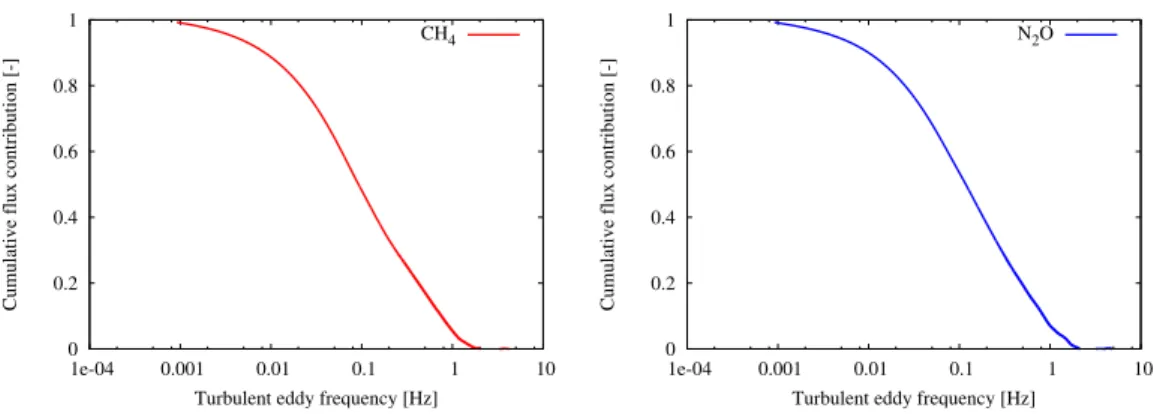
tributions of large eddies seeing that passive scalars, like CH₄ and N₂O, can acquire mesoscale fluctuations. These mesocale fluctuations can occure while the convective process, which drives their advection, itself fluctuates on a horizontal scale on the order of the boundary layer, i.e. within the microscale range (Jonker et al.,1999). An indica-tion of the underestimaindica-tion was made by means of ogive analyses based onLee et al.

25

(2004). The ogives of a neutral period on 7 Oktober 2006 between 12:00–14:00 are given in Fig.2. These ogives were calculated using a block averaging and an averaging time of one hour.

(14)

BGD

Full Screen / Esc

EGU smaller than 10% during this period. Besides, it was proved that an averaging time

of 30 min was long enough in this case. However, more research should be done to derive the amount of underestimation due to the running mean and the minimal required averaging time for all circumstances.

Calibrations have to be performed to improve the accuracy of the mixing ratio

val-5

ues and therefore the accuracy of the flux values. Nineteen calibration sessions were performed during two weeks, these were used for evaluating the difference between low, high and low-high calibrations. The standards were 1700 and 5100 ppb for CH₄ and 300 and 610 ppb for N2O (Scott speciality gasses, Netherlands). Three different

correction factors were calculated a low, a high and a low-high calibration factor. The

10

low-high calibration was defined by Eq. (2) and both other factors were determined by

fL= SL ML (10) fH= SH MH . (11)

The corrected concentration was found using one of these factors and the following equation

15

Ccor= fxCuncor (12)

withfx the low, high or low-high calibration factor,Cuncorthe uncorrected concentration

value in ppb andC_cor the corrected concentration value in ppb. The average and the standard deviation of the calibrations are given in Table3.

Table 3 shows a significant difference in all three correction factors. The low-high

20

calibration factor was the best way to estimate the NEE of CH₄and N₂O. A single point calibration with one-standard can provide flux values that differ by up to 16% from a two-standard estimate. The calibration factor changed when instrument parameters were modified and when changes were made in fitting parameters or in alignment. These kinds of modifications were the main reason for the standard deviation in each of the

(15)

BGD

Full Screen / Esc

EGU factors listed in Table3. It was also very important to keep the cell pressure constant

during the measurement and the calibration, since a pressure change affected the zero offset. This offset was due to a shift in baseline structure. To minimize this effect a better match than 0.1 Torr was required.

4.2 Methane and Nitrous oxide exchange rates

5

4.2.1 Analysis using 30-min flux values

A dataset of CH₄and N₂O EC-measurements had been obtained from 17 August to 6 November 2006 for which 99.8% was within the footprint of the investigated dairy farm site. About 7% of the CH4 and 22% of the N2O flux values were rejected by the

insta-tionarity tests (Foken and Wichura,1996). However, the averaged standard deviations

10

over six 5-min flux values were 84% and 185% for CH₄and N₂O, respectively. So, the temporal variation was very large for both greenhouse gases and especially for N2O.

The accepted and calibrated 30-min NEE values are shown in Fig.3.

In general the measurements for both CH₄ and N₂O show a net emission. About 97% and 86% of all flux values are positive for CH4 and N2O, respectively. In

con-15

sequence, also negative fluxes occurred which is an interesting result, however, the reliability should be analyzed in more detail to investigate if these fluxes were not caused by an instrumental artifact. Most fluxes were between –1000 ngC m−2s−1 and 1000 ngC m−2s−1 for CH4 or between –100 ngN m−2s−1and 100 ngN m−2s−1 for N2O.

The high positive peaks were clearly related to cow manure application. However, the

20

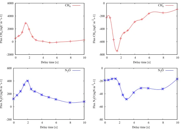
negative fluxes occurred in short events lasting at most a few hours. The reliability of the fluxes was checked using correlation versus delay time plots, see Fig.4for a pos-itive and a negative CH₄ and N₂O flux. These correlation plots suggested that these fluxes were well defined.

Furthermore, the detection limit of the QCL was estimated at 121 ngC m−2s−1 and

25

3 ngN m−2s−1based on the flux of 14 September 2006 21:00 using a method proposed by Wienhold et al. (1995). In this method, the standard deviation of the covariance

(16)

BGD

Full Screen / Esc

EGU function far outside the true lag time is used as the estimation. So, the estimated

detection limit was probably most of the time much smaller than the measured CH4

and N2O fluxes.

Besides instrumental artifacts, the negative fluxes could be caused by the non-performed Webb-correction (Webb et al.,1980). The Webb-correction for density

fluc-5

tuations should not apply to our fluxes since there was a constant temperature and pressure in the sampling cell. However, the Webb-correction for the influence of wa-ter vapour fluctuations on trace gas fluxes should be applied on the data seeing that the sample was not dried to a constant humidity before the mixing ratio was measured. The average magnitude of the Webb-correction for water vapour may be estimated from

10

the latent heat fluxes. When assuming a maximal and minimal latent heat flux of about 1000 and –400 W m−2, the maximal Webb-corrections are 484 and –194 ngC m−2s−1 and 188 and –75 ngN m−2s−1 for CH4 and N2O, respectively. So, a source above

194 ng C m−2s−1 and 75 ngN m−2s−1 can not change into a sink and a sink below – 484 ngC m−2s−1 and –188 ngN m−2s−1 can not change through the Webb-correction

15

into a source. An estimation of the corrected fluxes through the Webb-correction was performed using latent heat flux data of the University of Wageningen. These latent heat fluxes were also derived using eddy covariance data at a measurement height of about 3m at the same site. For more information about these measurements the reader is referred to Veenendaal et al. (2007)1. Still, 14% and 5% of all fluxes were

20

negative for CH4and N2O after applying this correction.

The conclusion is that large emissions of CH4and N2O occurred at this dairy farm on

peat grasslands. Moreover, negative emissions seemed to occur, however, more anal-yses should be performed to ascertain these uptakes. For the net annual exchange, the uptake episodes were negligible.

25

4.2.2 Analysis using week flux values

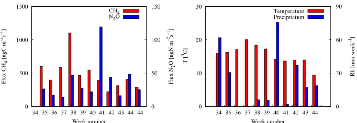
Week average flux values were calculated when data coverage higher than 50% oc-curred in more than four days a week. An overview of week averaged CH₄ flux and

(17)

BGD

Full Screen / Esc

EGU N₂O flux are presented in Fig.5. The week average air temperature and the weekly

precipitation rates are also shown in Fig.5. These have been made available by KNMI in the Netherlands. Cow manure was applied in week 37. It can be seen that the highest CH₄week average also occurred in this week. However, the highest N₂O took place in week 40 after a large amount of precipitation.

5

4.2.3 Analysis using three months flux values

The average calibration-corrected NEE and the standard deviation in the average were 484±375 ngC m−2s−1 and 39±62 ngN m−2s−1 from which 40% of N₂O emission was due to the fertilizing event. Thus, the standard deviations were of the same order of the average flux values this was mainly caused by the fertilizing event The calibrated

10

NEE was about 25% and 44% higher than the non-calibrated NEE for CH₄and N₂O, respectively. The average calibration factors over these three months were even higher than the average calibration factors over the nineteen test calibrations, which were per-formed in two weeks (see Sect.4.1). This was probably due to changes in temperature and voltage which affected the laser line shape and line width. In consequence, it

15

proved to be very important to calibrate frequently.

The calibrated and Webb-corrected NEE was about 7% higher for CH₄ and 29% higher for N₂O than the calibrated non-corrected NEE. However, this Webb-correction was based on latent heat fluxes of an open path system which was located at the same height and at a distance of about 3 m from the closed path eddy covariance

20

system of CH₄ and N₂O. In consequence, the Webb-correction should only partially be applied seeing that the 25 m inlet tube of the closed eddy covariance system of CH4 and N2O attenuated the fluxes. In consequence, the difference between

Webb-corrected and unWebb-corrected would be smaller. Thus, the calibrated NEE values without Webb-correction seemed to be a good first estimation of the CH4and N2O exchange

25

at this dairy farm on peat land. A summary of non-calibrated NEE, calibrated NEE and, calibrated and Webb-corrected NEE is given in Table4.

(18)

BGD

Full Screen / Esc

EGU

5 Conclusions

A quantum cascade laser spectrometer was used for EC-measurements of CH4 and

N₂O. Evaluation of its performance was performed using laboratory tests and three months of field measurements at a dairy farm on peat grasslands in the Nether-lands. All four required criteria for EC-measurements related to continuity, sampling

5

frequency, precision and stationarity were first checked in the laboratory. The system was able to run continuously using an automatic liquid nitrogen filling system. A sam-pling frequency of 10 Hz was obtained using a 1 GHz PC system. A precision of 2.6 and 0.3 ppb Hz−1/2 was obtained for CH4 and N2O, respectively. However, this precision

was strongly dependent on the power on the detector and thus alignment. Two-point

10

calibration was required at least once a week. Drift in the system was removed using a running mean filter of 120 s.

The continuous operation of the system was also proven by three months of field measurements (data coverage of 87%). A first indication of CH₄ and N₂O exchange was made. The average calibrated corrected exchange and its standard deviation was

15

484±375 ngC m−2s−1 and 39±62 ngN m−2s−1 from which 40% of N2O emission was

due to the fertilizing event. The N₂O peak, which was strongly correlated to precipi-tation, occured about three weeks after the fertilizing. Finally, although the dairy farm site was a net source of CH4 and N2O, also uptake seemed to occur in short events

lasting at most a few hours. However, more research should be done to investigate the

20

reliability of these negative fluxes.

In conclusion, a quantum cascade laser spectrometer was suitable for performing continuous EC-measurements of CH4 and N2O. Nevertheless, a two-point calibration

was necessary for obtaining accurate estimates. Besides, the possible underestimation due to the damping effect, the use of a running mean filter and the limited effective

25

sampling frequency should be analyzed in more detail.

Acknowledgements. This research was part of the Dutch National Research Program BSIK

(19)

BGD

Full Screen / Esc

EGU

T. Schrijver for their assistance during setting-up these experiments. We are also very grateful to E. Veenendaal of University of Wageningen for making available the latent heat flux data. Our thanks are also due to E. de Beus of Technical University of Delft for his assistance in data analyses. Finally, we owe a special debt of gratitude to the farmer T. van Eyk for using his farm site.

5

References

Allan, D. W.: Statistics of atomic frequency standards, Proceedings of the IEEE, 54, 221–230, 1966. 1147

Ammann, C.: On the applicability of relaxed eddy accumulation and common methods for measuring trace gas surface fluxes, Diss. ETH No. 12795, Zurich, 1998. 1146

10

Ammann, C., Brunner, A., Spirig, C., and Neftel, A.: Technical note: Water vapour concentration and flux measurements with PTR-MS, Atmos. Chem. Phys., 6, 4643–4651, 2006,

http://www.atmos-chem-phys.net/6/4643/2006/. 1145

Faist, J., Capasso, F., Sivco, D. L., Sirtori, C., Hutchinson, A. L., and Cho, A. Y.: Quantum cascade laser, Science, 264, 553–556, 1994. 1139

15

Foken, T. and Wichura, B.: Tools for quality assessment of surface-based flux measurements, Agric. Forest Meteorol., 78, 83–105, 1996.1146,1150

Hargreaves, K. J., Fowler, D., Pitcairn, C. E. R., and Aurela, M.: Annual methane emission from Finnish mires estimated from eddy covariance campaign measurements, Theor. Appl. Climatol, 70, 203–213, 2001. 1139

20

Hoogendoorn, C. J. and van der Meer, T. H.: Fysische transportverschijnselen II, Delftse Uit-gevers Maatschappij, Delft, The Netherlands, 1991.1143

IPCC: Climate change 2001, The Scientific Basis, Cambridge University Press, Cambridge, UK, 2001. 1138

IPCC: Climate change 1995, Scientific and technical analyses of impacts, adaptations and

25

mitigation. Contribution of working group II to the Second Assessment Report of the Inter-governmental Panel on Climatic Change, Cambridge University Press, London, 2006. 1138

Jim ´enez, R., Herndon, S., Shorter, J. H., Nelson, D. D., McManus, J. B., and Zahniser, M. S.: Atmospheric trace gas measurements using a dual quantum-cascade laser mid-infrared ab-sorption spectrometer, Proceedings of SPIE, 5738, 318–331, 2005. 1139,1142

(20)

BGD

Full Screen / Esc

EGU

Jonker, H. J. J., Duynkerke, P. G., and Cuijpers, J. W. M.: Mesoscales fluctuations in scalars generated by boundary layer convection, J. Atmos. Sci., 56, 801–808, 1999. 1148

Kaimal, J. C. and Finnigan, J. J.: Athmospheric boundary layer flows, Oxford University Press, Oxford, 1994. 1148

Kormann, R. and Meixner, F. X.: An analytical footprint model for non-neutral stratisfication,

5

Boundary-Layer Meteorology, 99, 207–224, 2001. 1146

Laville, P., Jambert, C., Cellier, P., and Delmas, R.: Nitrous oxide fluxes from a fertilized maize crop using micrometeorological and chamber methods, Agric. Forest Meteorol., 96, 19–38, 1999. 1139

Lee, X. L., Massman, W., and Law, B.: Handbook of micrometeorology, Kluwer Academic

10

Publishers, Dordrecht, The Netherlands, 2004.1144,1148

Lenschow, D. H. and Mann, J.: How long is long enough when measuring fluxes and other turbulent statistics?, Journal of Atmospheric and Oceanic Technology, 11, 661–673, 1994.

1145

McMillen, R. T.: An eddy correlation technique with extended applicability to non-simple terrain,

15

Boundary-Layer Meteorol., 43, 231–245, 1988.1143

Monteith, J. L. and Unsworth, M. H.: Principles of environmental physics, Edward Arnold, Lon-don, 1990.1139

Nelson, D. D., Shorter, J. H., McManus, J. B., and Zahniser, M. S.: Sub-part-per-billion detection of nitric oxide in air using a thermoelectrically cooled mid-infrared quantum cascade laser

20

spectrometer, Applied Physics B, 75, 343–350, 2002.1139,1142

Nelson, D. D., McManus, B., Urbanski, S., Herndon, S., and Zahniser, M. S.: High precision measurements of atmospheric nitrous oxide and methane using thermoelectrically cooled mid-infrared quantum cascade lasers and detectors, Spectrochimica Acta Part A, 60, 3325– 3335, 2004. 1139,1142,1146,1148

25

Nieuwstadt, F. T. M.: Turbulentie, Epsilon Uitgaven Utrecht, Utrecht, The Netherlands, 1998.

1143

Rothman, L. S. and Barbe, A.: The HITRAN molecular spectroscopic database: edition of 2000 including updates through 2001, Journal of Quantitative Spectroscopy and Radiative Transfer, 82, 5–44, 2003.1142

30

Smith, K. A., Clayton, H., Arah, J. R. M., Christensen, S., Ambus, P., Fowler, D., Hargreaves, K. J., Skiba, U., Harris, G. W., Wienhold, F. G., Klemedtsson, L., and Galle, B.: Micromete-orological and chamber methods for measurement of nitrous oxide fluxes between soils and

(21)

BGD

Full Screen / Esc

EGU

the atmosphere: Overview and conclusions, J. Geophys. Res., 99, 16 541–16 548, 1994.

1139

Webb, E. K., Pearman, G. I., and Leuning, R.: Correction of flux measurements for density effects due to heat and water vapour transfer, Q. J. R. Meteorol. Soc. 106, 85–100, 1980.

1151

5

Werle, P. and Kormann, R.: Fast chemical sensor for eddy-correlation measurements of methane emissions from rice paddy fields, Appl. Opt., 40, 846–858, 2001.1139

Werle, P. and Slemr, F.: Signal-to-noise ratio analysis in laser absorption spectrometers using optical multipass cells, Applied Optics, 30, 430–434, 1991.1147,1148

Wienhold, F. G., Frahm, H., and Harris, G. W.: Measurements of N₂O fluxes from fertilized

10

grassland using a fast response tunable diode laser spectrometer, J. Geophys. Res., 99, 16 557–16 567, 1994. 1139

Wienhold, F. G., Welling, M., and Harris, G. W.: Micrometeorological measurement and source region analysis of nitrous oxide fluxes from an agricultural soil, Atmos. Environ., 29, 2219– 2227, 1995. 1150

15

Wysocki, G., Kosterev, A. A., and Tittel, F. K.: Spectroscopic trace-gas sensor with rapidly scanned wavelenghts of a pulsed quantum casacade laser for in situ NO monitoring of in-dustrial exhaust systems, Appl. Phys. B, 80, 617–625, 2005. 1148

(22)

BGD

Full Screen / Esc

EGU

Table 1. Main characteristics of Oukoop site in Reeuwijk based on e.g. Veenendaal et

al. (2007)1.

Site Oukoop in Reeuwijk (NL) Location N 52◦01′15′′E 4◦01′17′′ Elevation of the polder (m below sea level) 1.6–1.7

Elevation of the ditches (m below sea level) 2.31–2.39 Height of vegetation (m) 0.15 Mean annual rainfall over 2004 and 2005 (mmyr−1) 870 Mean temperature over 2004 and 2005 (◦C) 10.3 Cow manure application in 2006 (m3ha−1) 55 Artificial fertilizer application in 2006 (kgha−1) 320

(23)

BGD

Full Screen / Esc

EGU

Table 2. Measurement precision (ppbHz−1/2) for ambient CH₄and N₂O with a cell pressure of

about 60Torr.

V∼80 mV V∼180 mV CH₄ 10 2.6 N₂O 1 0.3

(24)

BGD

Full Screen / Esc

EGU

Table 3. Average and standard deviation of nineteen calibration sessions which are performed

during two weeks.

Component f_L[–] f_H[–] f_LH[–] CH₄ 1.04±0.04 1.14±0.03 1.20±0.06 N₂O 1.03±0.06 1.07±0.05 1.12±0.05

(25)

BGD

Full Screen / Esc

EGU

Table 4. Average and its standard deviation of CH₄ and N₂O exchange at a dairy farm in the

Netherlands over the period 17 August to 6 November 2006.

CH₄[ngC m−2s−1] CH₄[mg m−2h−1] N₂O [ngN m−2s−1] N₂O [mgm−2h−1]

NEE non-calibrated without Webb-correction 388±275 1.86±1.32 27±42 0.15±0.24

NEE calibrated without Webb-correction 484±375 2.32±1.80 39±62 0.22±0.35

(26)

BGD

Full Screen / Esc

Printer-friendly Version Interactive Discussion EGU 0 0.2 0.4 0.6 0.8 1 0.01 0.1 1 10

Cumulative flux contribution [-]

Turbulent eddy frequency [Hz] CH4 T 0 0.2 0.4 0.6 0.8 1 0.01 0.1 1 10

Turbulent eddy frequency [Hz] N2O

T

Fig. 1. Comparison of the ogives of the sensible heat and CH₄flux (left) and of the sensible heat

and N₂O flux (right). The given ogives represent averages over 4 half-hourly measurements on 7 Oktober 2006 between 12:00–14:00.

(27)

BGD

Full Screen / Esc

Printer-friendly Version Interactive Discussion EGU 0 0.2 0.4 0.6 0.8 1 1e-04 0.001 0.01 0.1 1 10

Turbulent eddy frequency [Hz] CH4 0 0.2 0.4 0.6 0.8 1 1e-04 0.001 0.01 0.1 1 10

Turbulent eddy frequency [Hz] N2O

Fig. 2. Ogives of CH₄ flux (left) and N₂O flux (right) for determining the effect of the running

mean filter and averaging time. The given ogives represent averages over 2 one-hourly mea-surements on 7 Oktober 2006 between 12:00–14:00.

(28)

BGD

Full Screen / Esc

Printer-friendly Version Interactive Discussion EGU -2500 0 2500 5000 15/08 29/08 12/09 26/09 10/10 24/10 07/11 Flux CH 4 [ngC m -2s -1] Date -250 0 250 500 15/08 29/08 12/09 26/09 10/10 24/10 07/11 Flux N 2 O [ngN m -2s -1] Date

Fig. 3. 30-min flux values of CH₄(left) and N₂O (right) from a dairy farm site in the Netherlands

(29)

BGD

Full Screen / Esc

Printer-friendly Version Interactive Discussion EGU -2000 0 2000 4000 6000 0 2 4 6 8 10 Flux CH 4 [ngC m -2s-1] Delay time [s] CH4 -800 -600 -400 -200 0 0 2 4 6 8 10 Flux CH 4 [ngC m -2s-1] Delay time [s] CH4 -200 0 200 400 600 0 2 4 6 8 10 Flux N 2 O [ngN m -2s-1] Delay time [s] N2O -80 -60 -40 -20 0 0 2 4 6 8 10 Flux N 2 O [ngN m -2s-1] Delay time [s] N2O

Fig. 4. Correlation versus delay time plots for the positive CH₄flux of 14 September 2006 21:00

(red crosses) and the positive N₂O flux of 3 Oktober 2006 21:30 (blue stars) in the left figures. Correlation versus delay time plots for the negative CH₄flux of 23 September 2006 06:30 (red crosses) and the negative N₂O flux of 6 September 2006 13:00 (blue stars) in the right figures.

(30)

BGD

Full Screen / Esc

Printer-friendly Version Interactive Discussion EGU 0 500 1000 1500 34 35 36 37 38 39 40 41 42 43 44 44 0 50 100 150 Flux CH 4 [ngC m -2s -1] Flux N 2 O [ngN m -2s -1] Week number CH4 N2O 0 10 20 30 34 35 36 37 38 39 40 41 42 43 44 0 30 60 90 T [ 0C] Rh [mm week -1] Week number Temperature Precipitation

Fig. 5. Week average of CH₄ flux (left columns in red) and week average of N₂O flux (right

columns in blue) in left figure and week average of air temperature (left columns in red) and weekly precipitation rates (right columns in blue) in right figure.