Defining the climatic signal in stream salinity trends using the Interdecadal Pacific Oscillation and its rate of change

HAL Id: hal-00298775

https://hal.archives-ouvertes.fr/hal-00298775

HAL is a multi-disciplinary open access

archive for the deposit and dissemination of sci-entific research documents, whether they are pub-lished or not. The documents may come from teaching and research institutions in France or abroad, or from public or private research centers.

L’archive ouverte pluridisciplinaire HAL, est destinée au dépôt et à la diffusion de documents scientifiques de niveau recherche, publiés ou non, émanant des établissements d’enseignement et de recherche français ou étrangers, des laboratoires publics ou privés.

Defining the climatic signal in stream salinity trends

using the Interdecadal Pacific Oscillation and its rate of

change

V. H. Mcneil, M. E. Cox

To cite this version:

V. H. Mcneil, M. E. Cox. Defining the climatic signal in stream salinity trends using the Interdecadal Pacific Oscillation and its rate of change. Hydrology and Earth System Sciences Discussions, European Geosciences Union, 2006, 3 (5), pp.2963-2990. �hal-00298775�

HESSD

Full Screen / Esc

Printer-friendly Version Interactive Discussion Hydrol. Earth Syst. Sci. Discuss., 3, 2963–2990, 2006

www.hydrol-earth-syst-sci-discuss.net/3/2963/2006/ © Author(s) 2006. This work is licensed

under a Creative Commons License.

Hydrology and Earth System Sciences Discussions

Papers published in Hydrology and Earth System Sciences Discussions are under open-access review for the journal Hydrology and Earth System Sciences

Defining the climatic signal in stream

salinity trends using the Interdecadal

Pacific Oscillation and its rate of change

V. H. McNeil1and M. E. Cox2

1

Resource Sciences and Knowledge, Department of Natural Resources, Mines and Energy, Brisbane, Qld, Australia

2

School of Natural Resource Sciences, Queensland University of Technology, Brisbane, Qld, Australia

Received: 27 March 2006 – Accepted: 14 July 2006 – Published: 20 September 2006 Correspondence to: V. H. McNeil ([email protected])

HESSD

Full Screen / Esc

Printer-friendly Version Interactive Discussion Abstract

The impact of landuse on stream salinity is difficult to separate from decadal climatic variability, as the decadal scale climatic cycles in ground water and stream hydrology have similar wavelengths to the landuse pattern. These hydrological cycles determine the stream salinity through accumulation or release of salt in the landscape. The

In-5

terdecadal Pacific Oscillation (IPO) has been investigated before as an indicator of hydrological and related time series in the southern hemisphere. This study presents a new approach, which uses the rate of change in the IPO, rather than just its absolute value, to define an indicator for the climate component of ambient shallow groundwa-ter tables and corresponding stream salinity. Representative time series of wagroundwa-ter table

10

and stream salinity indicators are compiled, using an extensive but irregular database covering a very wide geographical area. These are modelled with respect to the IPO and its rate of change to derive climatic indicators. The effect of removing the decadal climatic influence from stream salinity trends is demonstrated.

1 Introduction 15

Variations or trends in salinity represented by Electrical Conductivity (EC) are often measured in streams and have the potential to be used as an indicator of landuse sus-tainability. Such measurements are relatively low cost and are convenient to automate; they also give important insights into the incipient development of dryland salinity, im-pacts of land clearing, irrigation, drainage alterations, and urbanisation. However, such

20

sources can only be relied on to define human impacts if they can be differentiated from variations that result from broad climate fluctuations.

The state of Queensland encompasses a considerable land area. It extends from 9◦S to 29◦S in latitude, and from 138◦E to 154◦E in longitude, and occupies most of the northeast quadrant of Australia. The influence of climatic fluctuations on stream salinity

25

was demonstrated when conductivity trends were calculated for about 500 gauging sta-2964

HESSD

Full Screen / Esc

Printer-friendly Version Interactive Discussion tions throughout the state over a twenty year period between 1970 and 1990 (QDPI,

1994). The results revealed a complex but consistent trend pattern evident in many streams, despite a very diverse range of topography, geology and landuse. Subse-quently it was found that stream EC and shallow unconfined water tables are related to climatic indicators such as the Southern Oscillation Index (SOI) and Interdecadal

5

Pacific Oscillation (IPO) (McNeil and Cox, 2002).

It was conceptually reasonable that these trends were at least partly related to hy-drological regimes of ground and surface water interaction. Salt is released into catch-ments through weathering, precipitation and dry fallout. Losses occur through runoff, wind blown dust, or percolation through the soil to the water table. The balance

be-10

tween sources and sinks of salt may vary according to prevailing rainfall and tempera-ture patterns which control the dynamic interactions between ground and surface wa-ter. Queensland rainfall is exceptionally variable both temporally and spatially (Nicholls, 1988; Loewe and Radok, 1948), with cycles covering decadal time scales. Major floods are often followed by a period of dry years, which may terminate in a prolonged drought.

15

Baseflow is affected by groundwater and is generally more saline than overland flow, due to prolonged contact with weathering minerals, so it raises the average salinity of streams. It is hypothesised that a flood flushes accumulated salts from the surface and upper soil horizons, resulting in large flows of dilute surface water. The wet conditions also recharge the groundwater, which can result in a greater contribution of baseflow

20

over the next few drier years. If the dry period continues, baseflow is lost as water tables drop below the streambeds, a feature typical of alluvial aquifers. This causes the streams to become more ephemeral, surface water dominated, and consequently less saline. The declining salinity trend continues slowly, until the next flood event, when there is a sharp drop followed by the subsequent rise. This hypothesis would

25

be verified if water tables, streamflow, and stream salinity could be related to climatic variables in a manner consistent with the observed patterns of occurrence.

A clear link between climate and streamflow has been established by a number of authors including Chiew et al. (1998) and Lough (1991), but apart from Vaccaro

HESSD

Full Screen / Esc

Printer-friendly Version Interactive Discussion (1993) who reported groundwater levels to be sensitive to climatic variability, and Evans

et al. (2001) who related salt concentration in lakes to variation in the North Atlantic Oscillation (NAO), there have been few studies to date on the numerical relationship between decadal climate indicators and water tables or surface water salinity.

The purpose of this study is to verify that climatic trends are present in the records

5

of Queensland stream salinity and its associated hydrology, using a new approach which incorporates both the Interdecadal Pacific Oscillation (IPO) and its rate of change (∆IPO) to derive decadal scale climatic indicators.

2 Choice of climatic indicators

The influence of climate on hydrology and subsequently stream salinity is not solely

10

related to precipitation, because temperature and evapotranspiration affect runoff, soil moisture storage and ultimately groundwater levels (Chiew et al., 1998). Therefore a more general and geographically broadscale climate indicator is required than could be provided by local observations such as running means of rainfall.

The most commonly used general climatic indicator is the El Nino/Southern

Oscilla-15

tion Index phenomenon (ENSO/SOI). It has been linked to precipitation and streamflow throughout the world by Philander (1990) and others. In addition there are studies on many specific regions, for instance: USA (Gray, 1990; Kahya and Dracup, 1993; Zorn and Waylen, 1997); Peru (Henderson et al., 1990); New Zealand (McKerchar et al., 1996; McKerchar et al., 1998; Gordon, 1986; Mullan, 1995); Belgium (Gellens and

20

Roulin, 1998) and western Africa (Gray, 1990). A number of authors including McBride and Nicholls (1983), Ropelewski and Halpert (1987, 1989), Lough (1991), and Chiew et al. (1998) have indicated the effect of ENSO/SOI on Queensland’s rainfall. Chiew et al. (1998) and Lough (1991) also established that as in the case of rainfall, there was a clear link between Australian streamflow and the ENSO/SOI, but Lough (1991),

25

Cordery et al. (1993), Burt and Shahgedanova (1998), and Power et al. (1999; 2005) have all observed that the relationship of ENSO/SOI with hydrology over time is

HESSD

Full Screen / Esc

Printer-friendly Version Interactive Discussion nitely non-stationary. This leads to problems in fitting long term hydrological time series

based on the SOI alone, indicating that its interaction with other global climatic influ-ences should also be considered.

Other modes of climatic variability have been detected on decadal time scales that are controlled by Sea Surface Temperature (SST) anomaly patterns. These may be

5

more aligned than the rapidly fluctuating ENSO/SOI to the longer term trends required to extract the climate signal from landuse in natural systems. They have been identified through complex empirical orthogonal functions (CEOF) (Trenberth and Hurrel, 1994; Rowell and Zwiers, 1999; Zhang et al., 1997). CEOF is a statistical technique used to detect structure revealed by very slow decay of percent variance in noisy data. The

10

most significant climatic signals that have been identified to date by CEOF analysis of global SST data are a secular trend representing global warming (IPCC, 1996) and the Inter-decadal Pacific Oscillation (IPO) described by Folland et al. (1999, 2002a, 2002b) and Power et al. (1999, 1998). Similarities have been noted between the ENSO/SOI and the IPO, although they were derived independently (Folland et al., 2002a; 2002b).

15

The IPO has been proved to modulate ENSO/SOI climate variability in the Pacific re-gion. (Salinger et al., 2001; Power et al., 2005) In particular, during positive phases of the IPO (IPO>0.5) El Nino events are noted to be more common, whereas La Ni ˜na events tend to occur more under the negative IPO phase (≤0.5).

2.1 The rate of change of the IPO as a climatic indicator

20

Recent studies (Kiem et al., 2002; Kiem and Franks, 2004; Franks, 2002; Jones and Everingham, 2005) and (McKeon et al., 2004) have incorporated both the IPO and the ENSO/SOI in their analyses of climatic effects on hydrology by dividing the IPO into positive, negative and neutral phases as recommended by Power et al. (1999), and modelling the likelihood of events on ENSO/SOI separately within each phase.

25

However, a more continuous indicator was required to analyse the effect of climate on a time series. It was also decided that a simple climatic indicator would be desirable to model the effect on stream salinity and groundwater levels. Whereas the effect

HESSD

Full Screen / Esc

Printer-friendly Version Interactive Discussion of ENSO/IPO on stream flow has been well established as described above, there

have been few climatic studies on groundwater levels and associated stream salinity. It is expected that reasonable correlations based on a simple model would be more convincing than a more complex model with greater skill.

The Burdekin River is one of the biggest rivers in Queensland, and has a flow history

5

extending back to the 1920s. It is also reasonably indicative of general hydrological conditions over a wide area of Queensland (Allan, 1985). Figure 1 shows annual flows in the Burdekin compared with the record of the IPO. The IPO has been estimated since 1870, and appears to rise irregularly then fall rapidly in phases of approximately 50 years. At the present time, the long term (50 year) trend is rising. It is apparent that

10

the general conditions of flow, particularly as indicated by the 3 year geometric mean, can be related to the behaviour of the IPO. Flows tend to be above the median when the IPO is changing rapidly, particularly when it is rising. As the rate of change slows, flows diminish, and droughts are most common when the rate of change is close to static. On the other hand, very high flows can occur, sometimes anomalously, when

15

a rapid slowing of the IPO leading to a change in direction takes place. Examples of such events are 1928, 1935, 1941, 1950–51, 1959, 1973–75, 1982, 1992, and 2001. Table 1 lists the expected stream flow according to the behaviours of the IPO. The similarity was considered sufficient to trial the IPO and its rate of change as the sole indicators to test for climatic variability in stream salinity and water levels.

20

3 Representative time series to model the climate signal

3.1 Data used in the study

The data used in this study are from the hydrological and chemical databases held by the Queensland Department of Natural Resources, Mines and Water (NRMW). Al-though these data are variable in content, reliability and periodicity of sampling, it was

25

expected that these would be evened out by the use of monthly medians which took 2968

HESSD

Full Screen / Esc

Printer-friendly Version Interactive Discussion account of the whole population. The surface water quality database contains nearly

50 000 EC measurements, collected from the 815 gauging stations since about 1962. The average number of samples per site is around 70, usually collected about four times a year. Some streamflow records date back to about 1920.

The groundwater data base contains about 500 000 individual water level (WL)

mea-5

surements from over 30 000 bores, most of which were only sampled once or twice, usually when first drilled. Although shallow groundwater is used throughout the state, the great majority of bores are concentrated in irrigated alluvial plains which have mostly been cleared and developed. Bores are particularly concentrated within irriga-tion areas, and therefore at risk of interference from pumping or regional depression,

10

or rises due to deforestation, watering, or disturbance to natural drainage patterns. 3.2 Producing annual time series for EC, water levels, and climate indicators

Time series were produced from monthly medians of EC and water tables shallower than about 30 m. All non-artesian WL measurements no deeper than 30 m, and all EC measurements taken at gauged sites within the particular month were included,

15

regardless of location. Annual time series were based on the climatic years (October of the preceding year through to September) to avoid splitting the (Southern Hemisphere) summer wet season, as recommended by Loewe and Radok (1948). Annual values were calculated if all months were represented for the climatic year. The arithmetic mean was used in the case of WL, and the geometric means in the case of EC, in line

20

with observed distributions. Finally, a smoothing technique (3 year moving geometric mean) was used to produce series in which seasonal variation was smoothed and the impact of irregularity and outliers minimised.

This exercise produced an almost continuous annual time series for EC since 1960, and WL since about 1950, but not all years were considered to be sufficiently

repre-25

sentative for use in constructing the climatic model. The representative time series contained only years with a reasonably comprehensive and consistent coverage of the state, and at leat 200 measurements in the case of EC, and 1000 in the case of

HESSD

Full Screen / Esc

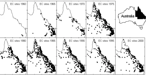
Printer-friendly Version Interactive Discussion water. Figure 2 summarises the distribution of EC measurement sites in Queensland

over the period of record. The representative period for modelling was taken as 1971– 2002 for EC, and 1968–2001 for WL. It is accepted that the distribution of gauging stations shown on Fig. 2 indicates that the EC time series would be most representa-tive of the coastal and central regions. However, the similarity of the pattern with that

5

observed throughout the state in QDPI (1994) indicates that it is general enough for a preliminary study aimed at verifying the existence of climatic influence in the trends rather than closely defining them. The pattern also resembles plots prepared by Jolly and Chin (1991) for bores in undisturbed areas of the Northern Territory to the west of Queensland which have been monitored since the 1950s.

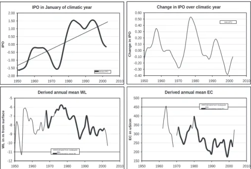
10

The January value of the slowly varying IPO was selected to represent the climatic year in the middle of the wet season. The∆IPO was taken as the difference between annual values. Figure 3 displays these climatic indicators with the EC and WL time series.

4 Modelling EC and water levels with the IPO and its rate of change 15

Modelling was carried out on the representative WL and EC time series through linear and second order polynomial regression with the IPO and its rate of change. Nonlinear-ity in the relationship between climatic indicators and hydrological time series has been noted by other authors such as Power et al. (2005). They pointed out that whereas the upper limits of hydrological events are not confined, lower limits are generally limited

20

The model was then applied to all years since 1950 in the case of WL and since 1960 in the case of EC.

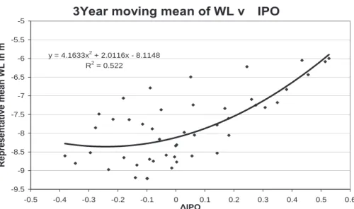
4.1 Groundwater levels

Modelling the WL time series was relatively simple. The first stage was a second order polynomial regression using the∆IPO (Fig. 3), which accounted for 50% of the total

25

HESSD

Full Screen / Esc

Printer-friendly Version Interactive Discussion variance. The equation is:

WL= 4.1633∆IPO2+ 2.0116∆IPO − 8.1148 (1)

The residuals from the first model were then plotted against the IPO to include the longer term trend. This produced the polynomial:

ResidualWL= 0.42IPO2− 0.47IPO − 0.3298. (2)

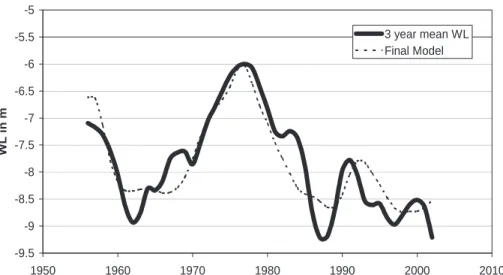
5

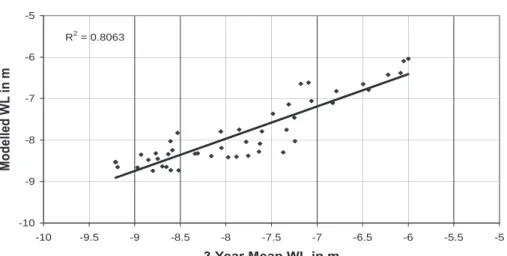
The final model of 3 years moving average water tables for bores less than 30 m was WL= 0.42IPO2− 0.47IPO+ 4.1633∆IPO2+ 2.0116∆IPO − 8.4446 (3) The correlation coefficient of the model with the time series 19, as shown on Fig. 4 was R2=0.81. Figure 5 compares the model and the WL series over time

4.2 Stream EC levels

10

Modelling the EC time series was less straightforward than the WL. For a start, the ∆IPO appears to vary stochastically about its median over the representative period, and the WL also displays little overall trend. However, as is clear from Fig. 2, the EC series, whilst similar in phase to the WL, shows a significant downward trend, in opposition to the upward trend shown by the IPO over the period. Walsh et al. (2002)

15

have also noted a decline in long term Queensland stream flows. Because stream salinity reflects the interactions between ground and surface waters, it was decided to first examine any component of the EC series that might be related to the long term gradient of the IPO. The period selected to reflect long term change was 50 years, 1950 to 2000, based on the apparent phases in the IPO. This trend was removed from

20

the EC data (available 1960 to 2000) by regression against the IPO trend, leading to the following equation, which accounted for 45% of the variance:

TrendinEC= −65.998 (1950 − CurrentYear) + 392.2. (4)

HESSD

Full Screen / Esc

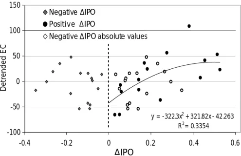
Printer-friendly Version Interactive Discussion The detrended EC, or residual component of the EC series, was then compared with

the∆IPO, as shown on Fig. 7. The series values for negative ∆IPO are also plotted with the∆IPO sign reversed. This plot shows the that the series is positively correlated with ∆IPO when ∆IPO is positive, but negatively correlated when ∆IPO is negative. This bimodal behaviour is understandable, because high residuals corresponding to low EC

5

occur during extreme rises and falls of the IPO, but low residuals are only conceptually likely when the IPO is approaching stability. This bimodality is related to the way that very wet conditions and very prolonged dry spells both reduce stream EC, as discussed in the Introduction. It is difficult to fit a simple algorithm to the untransformed series, but the reversed sign values fit sufficiently well with the positive values to indicate that the

10

rate of change of the IPO is sufficient to base the model on, regardless of the direction of change. Therefore, the detrended EC series was modelled on the absolute value of∆IPO using second order polynomial regression, which accounted for 34 percent of the remaining variance. The equation is:

DetrendedEC= −322.3 × |∆IPO|2+ 321.82 × |∆IPO| − 42.263 (5)

15

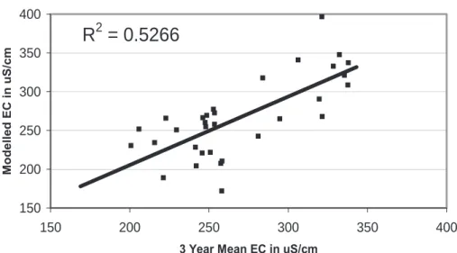
The final model was thus determined as:

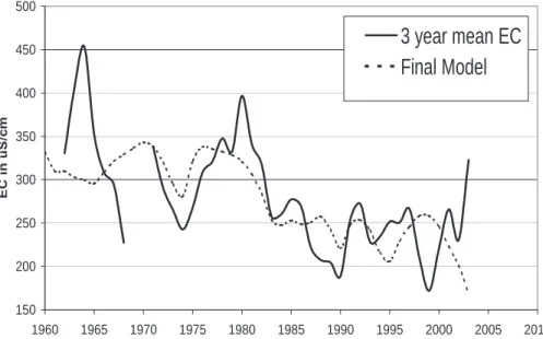
EC= −66 × (CurrentYear − 1950) − 322 × (|∆IPO|)2+ 322 × |∆IPO| + 350 (6) Figure 8 shows that this relationship has a correlation coefficient of over 50% (R2=0.53) with the 3-year moving average of EC measured at gauging stations. Figure 9 shows the model reasonably reflects EC trend direction in the years before 1970, where the

20

data was not sufficiently representative to be included in the model calibration. 4.2.1 Field evidence of the modelled climate signal

In the case of the WL representative series, it was found by McNeil and Cox (2002) that despite the effects of pumping, the average extensively measured bore shows a slight positive association with the climate indicator of just under 10%. In fact, 30% of

25

bores show a correlation of at least 30%, and more than 10% are over 50% correlated. 2972

HESSD

Full Screen / Esc

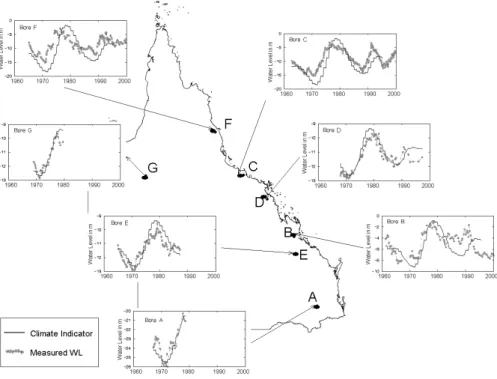
Printer-friendly Version Interactive Discussion Some examples of highly correlated water level records from various parts of the state

are shown on Fig. 10 from McNeil and Cox (2002) with the representative WL series (which has since been refined).

Recent studies have suggested that the EC records of many Queensland streams show a 10% to 50% correlation with the representative EC series, with downstream

5

catchments and shorter term periods (5 to 10 years) apparently being the most influ-enced by climatic cycles. Although the time series was derived predominantly from the southeast, the patterns in the series have also been found to be mirrored at various sites in most parts of the state, in continuance with those patterns observed in QDPI (1994). One such site was selected to trial the removal of climate trend from the EC

10

record.

5 The climate signal in stream salinity trends

The main objective of the study is the separation of landuse and climate EC trends using a representative control series in which the climatic signal had been verified. Because field EC data is collected several times a year and affected by season, the

15

monthly version of the representative EC series was preferred as the appropriate cli-mate control after being smoothed by a three month moving average. For testing, a gauging station with a long EC history was selected in a catchment which was exten-sively developed several decades ago. This was GS422316 on the Condamine River at Chinchilla, which has 117 EC readings collected between 1963 and 2004. These

20

readings were paired with the representative EC value for the closest date.

For this exercise, a test was required that would detect monotonic trend in stream EC records with non-normal distributions, seasonality and missing values. The rank based seasonal Kendall test defined by Hirsch et al. (1982) was selected, having been already trialled on a state-wide basis in QDPI (1994). Very large short term variability

25

occurs in stream EC simply from changes in flow, so it is removed from the data before a test for long term trend is applied. This was carried out using an algorithm derived

HESSD

Full Screen / Esc

Printer-friendly Version Interactive Discussion by Thorburn et al. (1992) which produces an S shaped curve based on the assumption

that the salinity will be asymptotic to that of the groundwater during baseflow, and to that of superficial runoff during high flood.:

EC= EC1− ECi 1+ BQ1/m

+ ECi (7)

where EC is salinity measured in the stream in µS/cm, EC₁is the median salinity under

5

lowest flow conditions, EC_i is the salinity approached by surface runoff during highest flows, Q is streamflow in m3s−1, and B and m are constants derived by optimisation.

A climate correction was then applied to the flow corrected data, based on linear regression with the representative ECs. The Kendall test was run on the flow corrected data, both with and without climate correction, with the results summarised on Fig.

10

11. Based on flow correction alone, there was a falling trend, with the null hypothesis of no trend being only 1% probable, but when the climate correction was added, no significant trend remained. A Spearman rank correlation between the site data and their paired monthly representative ECs gave a correlation coefficient of greater than 40%. This strongly suggests that the falling trend is climatic rather than related to the

15

local landuse, which has been stable in recent times.

6 Conclusions

A new approach has been demonstrated to define the climate signal in ambient ground-water level and stream salinity records, based on the rate of change of the IPO. Al-though this research is in its early stages, it is evident that such broadscale

represen-20

tative hydrological and stream salinity time series are useful for defining the medium and long term responses of natural systems to both climate and landuse. In future the control series might be refined to be more representative in space and time. Further mathematical analysis of the control series is needed to relate them more effectively to

HESSD

Full Screen / Esc

Printer-friendly Version Interactive Discussion climate processes. Also, back casting or extending the control time series, based on

historical or simulated climatic variables, would help assess the full natural ranges of parameters, or the likely impacts of future climatic conditions.

Acknowledgements. We thank the Department of Natural Resources, Mines and Water,

Queensland, for permission to use the water quality and groundwater databases and other 5

unpublished reports. We recognize the collective expertise in the department and thank our many colleagues for numerous stimulating and helpful discussions, including A. McNeil and R. Clarke. We also thank S. Choy and D. Begbie for their interest and encouragement of the project and J. Salinger for providing the IPO series from the UK Met. Office.

References 10

Allan, R. J.: The Australian summer monsoon, teleconnections and flooding in the Lake Eyre Basin. Adelaide, Royal Geographical Society of Australia, University of Adelaide Printing Section, 47, 1985.

Burt, T. P. and Shahgedanova, M.: An historical record of evaporation losses since 1815 calcu-lated using long-term observations from the Radcliffe Meteorological Station, Oxford, Eng-15

land, J. Hydrol., 205, 101–111, 1998.

Chiew, F. H. S., Piechota, T. C., Dracup, J. A., and McMahon, T. A.: El Nino/Southern Oscillation and Australian rainfall, streamflow and drought: Links and potential for forecasting, J. Hydrol., 204, 138–149, 1998.

Cordery, I., Yao, S. L., and Opoku-Ankomah, Y.: Forecasting drought – is it possible? In Hydrol-20

ogy and Water Resources Symposium Newcastle, NSW, Australia, 2 July–30 June, 387–391, 1993.

Evans, C., Montieth, D. T., and Harriman, R.: Long term variability in the deposition of marine ions at west coast sites in the U.K. Acid Waters Monitoring Network: impacts on surface water chemistry and significance for trend determination, Sci. Total Environ., 265, 115–129, 25

2001.

Folland, C. K., Parker, D. E., Colman, A. W., and Washington, R.: Large scale modes of ocean surface temperature since the late nineteenth century, in: Beyond El Nino: Decadal and interdecadal climate variability, edited by: Navarra, A., Ed. Berlin, Springer, 73–102, 1999.

HESSD

Full Screen / Esc

Printer-friendly Version Interactive Discussion

Folland, C. K., Renwick, J. A., Salinger, M. J., and Mullan, A. B.: Relative influences of the Interdecadal Pacific Oscillation and ENSO in the South Pacific Convergence Zone, Geophys. Res. Lett., 29, 21.21–21.24, 2002a.

Folland, C. K., Salinger, M. J., Jiangand, N., and Rayner, N. A.: Trends and Variations in South Pacific Island and Ocean Surface Temperatures, J. Climate, 16, 2859–2874, 2002b.

5

Franks, S. W.: Identification of a change in climate state using regional flood data, Hydrol. Earth Syst. Sci., 6, 11–16, 2002.

Gellens, D. and Roulin, E.: Streamflow response of Belgian catchments to IPCC climate change scenarios, J. Hydrol., 210, 242–258, 1998.

Gordon, N. D.: The Southern Oscillation and New Zealand weather, Monthly Weather Rev., 10

114, 371–387, 1986.

Gray, W. M.: Strong association between West African rainfall and U.S. landfall of intense hurricanes, Sci. Total Environ., 249, 1251–1256, 1990.

Henderson, K. A., Thompson, L. G., and Lin, P. N.: Recording of El Nino in ice core d18O records from Nevado Huascaran, Peru, J. Geophys. Res., 104, 31 053–31 065, 1990. 15

Hirsch, R. M., Slack, J. R., and Smith, R. A.: Techniques of trend analysis for monthly water quality data, Water Resour. Res., 18, 107–121, 1982.

IPCC: Report of the Intergovernmental Panel on Climate Change, edited by: Houghton, J. T., Callander, B. A., and Varney, S. K., Cambridge UK, Cambridge University Press, 1996. Jolly, P. B. and Chin, D. N.: Long term rainfall – recharge relationships within the Northern Terri-20

tory, Australia, In International Hydrology and Water Resources Symposium: The foundation for sustainable development Perth, W. A. Australia, 2–4 October, 1991.

Jones, K. and Everingham, Y.: Can ENSO combined with Low-Frequency SST signals enhance or suppress rainfall in Australian sugar growing areas?, in: MODSIM 2005 International Congress on Modelling and Simulation, edited by: Zerger, A., Argent, R. M., Melbourne, 25

December, Modelling and Simulation Society of Australia and New Zealand, 1660–1666, 2005.

Kahya, E. and Dracup, J. A.: U.S. streamflow patterns in relation to the El Nino/Southern Oscillation, Water Resour. Res., 29, 2491–2503, 1993.

Kiem, A. S., Franks, S. W., and Kuczera, G.: Multi-decadal variability of flood risk, Geophys. 30

Res. Lett., 30, 1035, Online access doi:1010.1029/2002GL015992, 012003.015999, 2002. Kiem, A. S. and Franks, S. W.: Multi-decadal variability of drought risk, eastern Australia,

Hy-drol. Processes, 18, 2039–2050, 2004.

HESSD

Full Screen / Esc

Printer-friendly Version Interactive Discussion

Loewe, F. and Radok, U.: Variability and periodicity of meteorological elements in the southern hemisphere with particular reference to Australia. Canberra, A.C.T., Commonwealth Meteo-rological Bureau, MeteoMeteo-rological Branch, Dept. of Interior, Commonwealth of Ausralia., 49, 1948.

Lough, J. M.: Rainfall variations in Queensland, Australia: 1891–1986, Int. J. Climatology, 11, 5

745–768, 1991.

McBride, J. L. and Nicholls, N.: Seasonal relationships between Australian rainfall and the Southern Oscillation, Monthly Weather Review, 111, 1998–2004, 1983.

McKeon, G. M., Hall, W. B., Henry, B. K., Stone, G. S., and Watson, I. W.: Pasture degradation and recovery in Australia’s rangelands: Learning from History, Queensland Department of 10

Natural Resources, Mines and Energy, 2004.

McKerchar, A. I., Pearson, C. P., and Moss, M. E.: Prediction of summer inflows to lakes in the Southern Alps, New Zealand, J. Hydrol., 184, 175–187, 1996.

McKerchar, A. I., Pearson, C. P., and Fitzharris, B. B.: Dependency of summer lake inflows and precipitation on spring SOI, J. Hydrol., 205, 66–80, 1998.

15

McNeil, V. H. and Cox., M. E.: Relationships between recent climate variation and water tables on stream salinity trends in northern Australia. In IAH International Groundwater Conference, Balancing the groundwater budget 12–17 May, Darwin, Northern Territory, 2002.

Mullan, A. B.: On the linearity and stability of Southern Oscillation-climate relationships for New Zealand, Int. J. Climatology, 15, 1365–1386, 1995.

20

Nicholls, N.: ENSO and rainfall variability, Journal of Climate, 1, 418–421, 1988.

Philander, S. G. H.: El Nino, La Nina and the Southern Oscillation, San Diego, Academic Press, 1990.

Power, S., Tseitkin, F., Torok, S., Lavery, B., Dahni, R., and McAvaney, B.: Australian temper-ature, Australian rainfall and the Southern Oscillation, 1910–1992: coherent variability and 25

recent changes, Australian Meteorological Magazine, 47, 85–101, 1998.

Power, S., Casey, T., Folland, C., Colman, A., and Mehta, V.: Inter-decadal modulation of the impact of ENSO on Australia, Climate Dynamics, 15, 319–324, 1999.

Power, S., Haylock, M., Colman, R., and Wang, X.: Asymmetry in the Australian response to ENSO and the predictability of inter-decadal changes in ENSO teleconnections. Melbourne 30

Australia, Bureau of Meteorology, 65, 2005.

QDPI: Queensland Water Quality Atlas, Brisbane, Queensland Department of Primary Indus-tries, 1994.

HESSD

Full Screen / Esc

Printer-friendly Version Interactive Discussion

Ropelewski, C. F. and Halpert, M. S.: Global and regional scale precipitation patterns associ-ated with the El Nino/Southern Oscillation, Monthly Weather Rev., 115, 1606–1626, 1987. Ropelewski, C. F. and Halpert, M. S.: Precipitation patterns associated with the high index

phase of the Southern Oscillation, J. Climate, 2, 268–284, 1989.

Rowell, D. P. and Zwiers, F. W.: The global distribution of sources of atmospheric decadal 5

variability and mechanisms over the tropical Pacific and southern North America, Climate Dynamics, 15, 751–772, 1999.

Salinger, M. J., Renwick, J. A., and Mullan, A. B.: Interdecadal Pacific Oscillation and South Pacific climate, Int. J. Climatology, 21, 1705–1721, 2001.

Thorburn, P., Shaw, R. and Gordon, I.: Modelling salt transport in the landscape, in: Modelling 10

chemical transport in soils, edited by: Gladiri, H. and Rose, C. W., Senir Publisher, 180–189, 1992.

Trenberth, K. E. and Hurrel: On the evolution of the Southern Oscillation, Monthly Weather Rev., 115, 3078–3096, 1994.

Vaccaro, J. J.: Sensitivity of groundwater recharge estimates to climate variability and change, 15

Columbia Plateau, Washington, J. Geophys. Res., 97, 2821–2833, 1993.

Walsh, K., Cai, W., Hennessy, K., Jones, R., McInnes, K., Nguyen, K., Page, C., and Whetton, P.: Climate change in Queensland under enhanced greenhouse conditions Final Report, 1997–2002, CSIRO Atmos. Res., 2002.

Zhang, Y., Wallace, J. M., and Battisti, D. S.: ENSO-like interdecadal variability: 1900–93, J. 20

Climate, 10, 1004–1020, 1997.

Zorn, M. H. and Waylen, P. R.: Seasonal response of mean monthly streamflow to El Nino/Southern Oscillation in North Central Florida, The Professional Geographer, 49, 51– 62, 1997.

25

HESSD

Full Screen / Esc

Printer-friendly Version Interactive Discussion

Table 1. Predictability of decadal flow trends in the Burdekin River, based on behaviour of the

IPO as illustrated in Fig. 1.

Decade Behaviour of the IPO Expected Burdekin flow regime.

1920–1930 Rising, quite rapidly in mid years At least median, above in mid years

1930–1940 Fall then rise, but fairly static Usually low, particularly in early years

1940–1950 Falling rapidly Above median

1950–1960 Rising, rapidly in later years Above median, particularly in later years

1960–1970 Stationary Very low

1970–1980 Slow fall early, then very rapid rise Low initially, then well above median

1980–1990 Slowing rise then slow fall Dropping and remaining below median

1990–2000 Slow rise followed by rapid fall Around median, driest in mid years

HESSD

Full Screen / Esc

Printer-friendly Version Interactive Discussion y = 0.0525x - 103.7 R2_{= 0.5447} -2 -1.5 -1 -0.5 0 0.5 1 1.5 2 1870 1880 1890 1900 1910 1920 1930 1940 1950 1960 1970 1980 1990 2000 2010 IP O 1000 00 1000 000 1000 0000 1000 0000 0 1870 1880 1890 1900 1910 1920 1930 1940 1950 1960 1970 1980 1990 2000 2010 C li m ati c year fl o w (M L ) Burdekin Flow Median IPO IPO since 1950

Linear Trend (IPO since 1950)

Three-year moving average

Fig. 1. Comparison of the long term IPO and recorded annual flows in the Burdekin River. The

tendency for the IPO to go through a generally rising and falling phase on about a 50 year cycle is observed, as well as the tendency for the river flow to be above the median when the IPO is changing rapidly, particularly when the change is positive.

HESSD

Full Screen / Esc

Printer-friendly Version Interactive Discussion

Fig. 2. Distribution of EC samples stored in the NRME database, representing Queensland

over time.

HESSD

Full Screen / Esc

Printer-friendly Version Interactive Discussion IPO in January of climatic year

-2.00 -1.50 -1.00 -0.50 0.00 0.50 1.00 1.50 2.00 1950 1960 1970 1980 1990 2000 2010 IPO January IPO

Change in IPO over climatic year

-0.40 -0.30 -0.20 -0.10 0.00 0.10 0.20 0.30 0.40 0.50 0.60 1950 1960 1970 1980 1990 2000 2010 C hange in IPO IPO

Derived annual mean WL

-12 -11 -10 -9 -8 -7 -6 -5 1950 1960 1970 1980 1990 2000 2010 WL in m from s urface

Estimated from inadaquate data Representative mean WL

Derived annual mean EC

150 200 250 300 350 400 450 500 1950 1960 1970 1980 1990 2000 2010 EC in u S/ cm

Estimated from inadaquate data Representative mean EC

Fig. 3. Climatic variables IPO and ∆IPO, and State-wide representative water tables and

stream salinity since 1950, as used for the modelling.

HESSD

Full Screen / Esc

Printer-friendly Version Interactive Discussion

3Year moving mean of WLv IPO

y = 4.1633x2_{+ 2.0116x - 8.1148} R2= 0.522 -9.5 -9 -8.5 -8 -7.5 -7 -6.5 -6 -5.5 -5 -0.5 -0.4 -0.3 -0.2 -0.1 0 0.1 0.2 0.3 0.4 0.5 0.6 IPO R e p rese n ta ti ve m ea n WL in m

Fig. 4. Groundwater levels modelled against∆IPO using nonlinear (quadratic) regression.

HESSD

Full Screen / Esc

Printer-friendly Version Interactive Discussion Mean WL v model based on the IPO and IPO

R2_{= 0.8063} -10 -9 -8 -7 -6 -5 -10 -9.5 -9 -8.5 -8 -7.5 -7 -6.5 -6 -5.5 -5 3 Year Mean WL in m M od e ll e d WL in m

Fig. 5. Three-year moving mean groundwater levels compared with the model based on the

IPO and its rate of change,∆IPO.

HESSD

Full Screen / Esc

Printer-friendly Version Interactive Discussion

Comparison of mean WLs and final model over time

-9.5 -9 -8.5 -8 -7.5 -7 -6.5 -6 -5.5 -5 1950 1960 1970 1980 1990 2000 2010 WL in m 3 year mean WL Final Model

Fig. 6. Three year moving mean groundwater levels compared with the model over time

verify-ing a broad scale climatic component in the series.

HESSD

Full Screen / Esc

Printer-friendly Version Interactive Discussion y = -322.3x2+ 321.82x- 42.263 R2= 0.3354 -100 -50 0 50 100 150 -0.4 -0.2 0 0.2 0. 4 0.6

IPO

Negative IPO absolute values

Fig. 7. EC residuals modelled against the absolute value of∆IPO using nonlinear (quadratic)

regression. The 3 year moving mean ECs were first detrended using the linear trend in the IPO since 1950.

HESSD

Full Screen / Esc

Printer-friendly Version Interactive Discussion

MeanECv model based on theIPOand IPO

R

= 0.5266

3 Year Mean EC in uS/cm

M od e ll e d E C in u S/ c m

Fig. 8. Three year moving mean ECs compared with the model based on the IPO and its rate

of change,∆IPO.

HESSD

Full Screen / Esc

Printer-friendly Version Interactive Discussion 150 200 250 300 350 400 450 500 1960 1965 1970 1975 1980 1985 1990 1995 2000 2005 2010 E C in u S/ c m

3 year mean EC

Final Model

Fig. 9. Three year moving mean EC levels compared with the model over time verifying a broad

scale climatic component in the series.

HESSD

Full Screen / Esc

Printer-friendly Version Interactive Discussion

Fig. 10. Selection of bore water level records showing influence of the climatic indicator over a

wide range of Queensland.

HESSD

Full Screen / Esc

Printer-friendly Version Interactive Discussion

Fig. 11. An example of a stream with an apparent falling EC trend, but with a general

pat-tern that resembled the derived climate indicator time series. When the effect of climate was removed by linear regression with the climate indicator, no significant trend remained.