HAL Id: hal-02337414
https://hal.sorbonne-universite.fr/hal-02337414
Submitted on 29 Oct 2019HAL is a multi-disciplinary open access
archive for the deposit and dissemination of sci-entific research documents, whether they are pub-lished or not. The documents may come from teaching and research institutions in France or abroad, or from public or private research centers.
L’archive ouverte pluridisciplinaire HAL, est destinée au dépôt et à la diffusion de documents scientifiques de niveau recherche, publiés ou non, émanant des établissements d’enseignement et de recherche français ou étrangers, des laboratoires publics ou privés.
the subpolar
L. Lacour, N. Briggs, Hervé Claustre, M. Ardyna, G. Dall’Olmo
To cite this version:
L. Lacour, N. Briggs, Hervé Claustre, M. Ardyna, G. Dall’Olmo. The intra-seasonal dynamics of the mixed layer pump in the subpolar. Global Biogeochemical Cycles, American Geophysical Union, 2019, 33 (3), pp.266-281. �10.1029/2018GB005997�. �hal-02337414�
The intra-seasonal dynamics of the mixed layer pump in the subpolar
1
North Atlantic Ocean: a BGC-Argo float approach.
2 3
L. Lacour1†, N. Briggs2, H. Claustre1, M. Ardyna1,3, G. Dall’Olmo4,5
4 5
1Sorbonne Université, CNRS, Laboratoire d’Océanographie de Villefranche, LOV, F-06230
6
Villefranche-sur-mer, France. 7
2National Oceanography Centre, European Way, Southampton SO14 3ZH, UK.
8
3Department of Earth System Science, Stanford University, Stanford CA 94305, USA.
9
4Plymouth Marine Laboratory, Prospect Place, The Hoe, Plymouth PL1 3DH, UK.
10
5National Centre for Earth Observation, Plymouth Marine Laboratory, Prospect Place, The Hoe,
11
Plymouth PL1 3DH, UK. 12
13
Corresponding author: Léo Lacour (leo.lacour@takuvik.ulaval.ca) 14
† Now at Takuvik Joint International Laboratory, CNRS and Université Laval, Québec, 15 G1V0A6, Canada. 16 17 Key Points: 18
• The density of BGC-Argo float network enables identification of episodic mixed layer 19
pump events on a basin-scale. 20
• Intra-seasonal dynamics of the mixed layer pump drives episodic inputs of fresh organic 21
material to the mesopelagic during the winter to spring transition. 22
• This mechanism provides a significant source of energy to the mesopelagic food-web 23
before the spring bloom period. 24
25
Abstract
26
The detrainment of organic matter from the mixed layer, a process known as the mixed layer 27
pump (ML pump), has long been overlooked in carbon export budgets. Recently, the ML pump 28
has been investigated at seasonal scale and appeared to contribute significantly to particulate 29
organic carbon export to the mesopelagic zone, especially at high latitudes where seasonal 30
variations of the mixed layer depth are large. However, the dynamics of the ML pump at intra-31
seasonal scales remains poorly known, mainly because the lack of observational tools suited to 32
studying such dynamics. In the present study, using a dense network of autonomous profiling 33
floats equipped with bio-optical sensors, we captured widespread episodic ML pump-driven 34
export events, during the winter and early spring period, in a large part of the subpolar North 35
Atlantic Ocean. The intra-seasonal dynamic of the ML pump exports fresh organic material to 36
depth (basin-scale average up to 55 mg C m-2 d-1), providing a significant source of energy to
37
the mesopelagic food web before the spring bloom period. This mechanism may sustain the 38
seasonal development of overwintering organisms such as copepods with potential impact on 39
the characteristics of the forthcoming spring phytoplankton bloom through predator-prey 40 interactions. 41 42 1 Introduction 43
The export of organic matter from the surface to the ocean interior has traditionally been 44
attributed to the gravitational settling of particulate organic carbon (POC), namely the 45
biological gravitational pump (Sanders et al., 2014; Siegel et al., 2016). The gravitational pump 46
at high latitudes is closely related to the spring phytoplankton bloom (Martin et al., 2011). Large 47
phytoplankton cells such as diatoms (> 20 µm) that thrive during the spring bloom contribute 48
significantly to the downward carbon flux due to their high sinking rate (up to 50 m d-1,
Villa-49
Alfageme et al., 2016), and their ability to form large aggregates (Smetacek, 1985, 1999). 50
Zooplankton also play a key role by repackaging organic matter into fecal pellets, thereby 51
enhancing the speed at which it sinks out of the euphotic zone (Turner, 2002, 2015). Up to 90% 52
of the exported material may be consumed and remineralized back into dissolved inorganic 53
carbon (DIC) by heterotrophic activity in the mesopelagic zone (~100 - 1,000 m; Buesseler & 54
Boyd, 2009; Kwon et al., 2009). Finally, a small fraction of this material may be sequestered in 55
the bathypelagic zone (> 1,000 m) on timescales of months to millennia (Ducklow et al., 2001; 56
Poulton et al., 2006). 57
In complement to the biological gravitational pump, Lévy et al. (2001), Omand et al. (2015) 58
and Llort et al. (2018) provided evidence that export of organic matter also occurs through 59
localized (1-10 km) eddy-driven subduction of non-sinking particles, and possibly dissolved 60
organic carbon (DOC). In subpolar oceans, the eddy-driven subduction pump may contribute 61
up to half of the total springtime export of POC (Omand et al., 2015). Through eddy-driven 62
stratification, these submesoscale processes can also enhance the production of organic matter 63
at the surface which will potentially be exported by subsequent eddy-driven subduction 64
(Mahadevan et al., 2012; Omand et al., 2015). Submesoscale subduction thus leads to episodic 65
injections of POC- and DOC-rich waters below the mixed layer, possibly outside the spring 66
bloom period. As current estimates of metabolic activity in the mesopelagic region exceed the 67
influx of organic substrates generally attributed to the biological pump (Burd et al., 2010; 68
Giering et al., 2014; Steinberg et al., 2008), submesoscale subduction has been invoked as an 69
alternate pathway allowing a better balance of the carbon budget (Barth et al., 2002; Lévy et 70
al., 2001; Omand et al., 2015). The spatial heterogeneity of this process could indeed stimulate 71
hotspots of organic substrates, likely missed by conventional sampling methods. 72
Recently, Dall’Olmo et al. (2016) highlighted the global impact on carbon export budgets of 73
seasonal detrainment of organic matter, a process known as the seasonal mixed layer pump (ML 74
pump). A few localized studies had first described this mechanism at the diurnal timescale, 75
showing that alternation of night convection and daily restratification can lead to an 76
entrainment-detrainment cycle of particles from the mixed layer (Gardner et al., 1995; Ho & 77
Marra, 1994; Woods & Onken, 1982). Indeed, the mixed layer deepens due to the effect of wind 78
and heat loss to the atmosphere (Price et al., 1986) but does not shoal smoothly, as commonly 79
assumed for the sake of simplicity. Instead, the upper-ocean stratifies due to solar heating or 80
other sources (e.g. freshwater flux, slumping of isopycnals) and eventually a new mixed layer 81
re-forms from the surface, thereby isolating phytoplankton cells and other particles in the so-82
called remnant layer (Franks, 2015; Ho & Marra, 1994; Fig. 1). At the diurnal timescale, the 83
amplitude of the mixing layer depth variation is small (Woods & Onken, 1982) and much of 84
the detrained organic material can be entrained back into the mixing layer. Thereby, the net 85
export of carbon by the ML pump is accordingly weak. At the seasonal scale, however, the ML 86
pump is a process of greater significance (Carlson et al., 1994; Dall’Olmo et al., 2016; 87
Dall’Olmo & Mork, 2014). In springtime, the seasonal stratification of deep mixed layers 88
contributes to export large amounts of carbon as dissolved organic matter or small non-sinking 89
particles. In high-latitude regions with deep winter mixing, the seasonal ML pump amounts on 90
average to 23% of the carbon supplied by fast sinking particles (Dall’Olmo et al., 2016). 91
The winter to spring evolution of the mixed layer depth (MLD) does not correspond to a smooth 92
shoaling but rather is interspersed with restratification and deep mixing events (Lacour et al., 93
2017). Such intermittent mixing can enhance both phytoplankton production and POC export 94
through the so-called intra-seasonal ML pump (Bishop et al., 1986; Garside & Garside, 1993; 95
Giering et al., 2016; Koeve et al., 2002). When detrainment fluxes exceed entrainment fluxes, 96
the intra-seasonal ML pump can lead to a net export of carbon to the mesopelagic. In the north-97
east Iceland basin, Giering et al. (2016) have shown that the pre-bloom flux of small particles 98
driven by the ML pump can be of similar magnitude to the total particle export rate by 99
sedimentation observed during, and after, the spring bloom period. However, the analysis of 100
long-term sediment trap data from 3000 m at the Porcupine Abyssal Plain (49°N, 16°W) 101
revealed that pre-bloom deep fluxes are small (Lampitt et al., 2010). This discrepancy suggests 102
that most of the particulate material exported by the ML pump is consumed in the mesopelagic 103
zone (Giering et al., 2016), and potentially ventilated back into the atmosphere the following 104
winter as inorganic carbon. Thus, this process may be less relevant to the long-term 105
sequestration of carbon than for supplying energy to the mesopelagic food-web. In particular, 106
zooplankton populations, especially overwintering organisms, inhabiting cold, dark and low 107
turbulence environments at depth (Jónasdóttir et al., 2015; Steinberg & Landry, 2017; Visser et 108
al., 2001) could benefit from the ML pump. 109
These three main pathways of carbon (i.e. the gravitational pump, the eddy-driven pump and 110
the mixed layer pump) all contribute to the biological carbon pump (Dall’Olmo et al., 2016; 111
Siegel et al., 2016; Llort et al., 2018). Indeed, they transfer organic matter from the productive 112
mixing layer to the ocean interior where light and mixing are reduced. The amount of exported 113
material determines the strength of the biological pump while the sequestration timescale 114
control its efficiency (Buesseler & Boyd, 2009). For the particular case of the intra-seasonal 115
ML pump, the strength is defined as the net amount of particulate organic carbon resulting from 116
an entrainment-detrainment cycle. 117
Despite the recent discoveries mentioned above, the intra-seasonal dynamics of the ML pump 118
and its potential role in sustaining mesopelagic ecosystems still remains poorly understood. The 119
reason is twofold. First, current methods to estimate the depth of the mixed layer are not 120
appropriate. Brainerd et al. (1995) highlighted the importance in distinguishing the mixed layer, 121
the zone of relatively homogenous water formed by the history of mixing, from the mixing 122
layer, the zone in which mixing is currently active. They showed that current density-derived 123
methods fail to capture the high-frequency variability of the mixing layer. Second, most existing 124
observational tools are not well suited to study such unpredictable episodic and widespread 125
events. Using high-frequency sampling from autonomous profiling floats equipped with bio-126
optical sensors, we investigate here the intra-seasonal dynamics of the ML pump in the subpolar 127
North Atlantic Ocean, a region that exhibits a strong spatiotemporal variability of the MLD. 128
More specifically, we attempt to quantify the strength of the intra-seasonal ML pump on a basin 129
scale, and characterize the nature and the fate of the exported material in the mesopelagic. The 130
efficiency of this process in terms of long-term sequestration of carbon is not addressed. Rather, 131
we discuss its importance in supplying pulses of fresh organic substrate to the mesopelagic 132
ecosystem. 133
2 Material and Methods
135
2.1 The BGC-Argo dataset: description and data processing
136
The data used in this study were acquired by a fleet of 14 BGC-Argo floats that were deployed 137
in the subpolar North Atlantic Ocean. These floats provided 2126 profiles spanning all seasons 138
between 2014 and 2016 (Fig. 2). These floats (NKE PROVOR CTS-4) were equipped with: an 139
SBE 41 CTD; a WET Labs ECO3 (Combined Three Channel Sensors) composed of a 140
chlorophyll a (Chla) fluorometer, a Colored Dissolved Organic Matter (CDOM) fluorometer, 141
and an optical backscattering sensor at 700 nm (bbp); and an OCR-504 radiometer measuring
142
Photosynthetically Available Radiation integrated over 400-700 nm (PAR). Measurements 143
were collected during ascent every 2, 5 or 10 days, from 1,000 m (parking depth) to the surface. 144
Vertical resolution of acquisition was 10 m between 1,000 m and 250 m, 1 m between 250 m 145
and 10 m, and 0.2 m between 10 m and the surface. Radiometric measurements were acquired 146
only in the upper 250 m. Data were transmitted through Iridium communication each time the 147
floats surfaced, usually around local noon. 148
A “real time” quality control procedure was performed on the CTD data (Wong et al., 2015), 149
Chla (Schmechtig et al., 2014) and PAR measurements (Organelli et al., 2016) after the factory 150
calibrations were applied. The instrumental dark signal was removed from the Chla profile 151
following the method in Xing et al. (2011) and the non-photochemical quenching (NPQ) was 152
corrected as follows: the maximum Chla value above MLD, defined as a density difference of 153
0.01 kg m-3 with a reference value at 5 m, is extrapolated toward the surface. As an additional
154
condition, the depth of the extrapolated Chla value has to be shallower than the depth of the 155
isolume 20 µmol photons m-2 s-1 (derived from smoothed PAR profile), which marks
156
approximatively the lower limit of the potential NPQ effect for mixed waters in this area 157
(Lacour et al., 2017; Xing et al., 2018). Chla values were divided by a factor of 2 to account for 158
a calibration systematic error in Wet Labs fluorometers (Roesler et al., 2017). Spikes were 159
removed from Chla and bbp profiles using a 5-point running median filter and a 7-point running
160
mean filter similar to Briggs et al. (2011). The spike signals from bbp profiles were used to
161
detect large particles or aggregates following Briggs et al. (2011). Note that, because of the 162
lower vertical resolution sampling below 250 m, deep spikes are not well resolved which 163
potentially leads to an underestimation of large particles and aggregates. For the same reason, 164
the depth correction for carbon loss relative to bbp in aggregates used by Briggs et al. (2011)
165
was not applied. Both baseline and spike signals from bbp profiles were converted into POC
166
using an empirical factor of 37,537 mg POC m-2 in the mixing layer and 31,519 mg POC m-2
167
below (Cetinić et al., 2012). This relationship might be biased by a background bbp signal that
is not necessarily related to POC. Consequently, before converting to POC, the median of deep 169
(950-1,000 m) bbp values measured by each float was subtracted from each profile of the
170
corresponding time series. POC derived from the baseline bbp signal likely corresponds to small
171
particles (0.2-20 µm; Dall’Olmo & Mork, 2014) whereas POC derived from spike signal 172
corresponds to large particles or aggregates (Briggs et al., 2011). When not used as POC 173
proxies, bbp profiles are presented without the correction described above (i.e. removing deep
174 values). 175 176 2.2 Atmospheric data 177
Net heat flux data were extracted from the ECMWF ERA Interim data set (reanalysis), freely 178
available at http://apps.ecmwf.int/datasets/data/interim-full-daily/levtype=sfc. These data were 179
averaged over 24-hour periods, with spatial resolution of 0.25°. 180
Wind stress data were extracted from the Ifremer CERSAT Global Blended Mean Wind Fields 181
data set, freely available at http://marine.copernicus.eu/. This data set was estimated from 182
scatterometers ASCAT and OSCAT retrievals and from ECMWF operational wind analysis 183
with a horizontal resolution of 0.25° and 6 hours in time. Wind stress data were subsequently 184
averaged over 24-hour periods to match net heat flux data. Wind stress 𝜏 was used to calculate 185
the Ekman vertical length scale as follows: 𝑍𝐸𝑘 = 𝛾 𝑤𝑓∗ , where 𝛾 is an empirical constant of 186
0.5 (Wang & Huang, 2004), 𝑓 = 2 × 7.29 × 10−5× 𝑠𝑖𝑛(𝑙𝑎𝑡𝑖𝑡𝑢𝑑𝑒) is the Coriolis parameter
187
and 𝑤∗ is the turbulent friction velocity 𝑤∗ = √𝜌𝜏
𝑤 with 𝜌𝑤 the density of the surface water.
188 189
2.3 Estimation of mixing and mixed layer depths
190
A single criterion, the maximum vertical gradient, was used to estimate the mixing and mixed 191
layer depths from Chla (maximum negative gradient) and density profiles (maximum positive 192
gradient), respectively. To suppress the influence of spikes or noise, these profiles were 193
additionally smoothed (Butterworth filter) before calculating the maximum gradient and the 194
NPQ correction, which may erase a potential gradient, was performed after calculating the 195
maximum gradient. 196
The maximum density gradient (MLDdens) is interpreted to match the depth of the seasonal
197
pycnocline (i.e. mixed layer depth), which is the envelope of the maximum depth reached by 198
the mixing layer (Brainerd & Gregg, 1995). In contrast, the maximum Chla gradient (MLDbio)
199
should mark the mixing layer depth with time scales typical of phytoplankton growth (Boss & 200
Behrenfeld, 2010; Zawada et al., 2005) (Fig. 1). The underlying concept is that Chla is 201
homogeneous over the whole mixing layer, if turbulent mixing overcomes vertical variations 202
in the phytoplankton net growth rate (Huisman et al., 1999; Taylor & Ferrari, 2011). Indeed,
203
while phytoplankton cells grow within the euphotic layer, mixing redistributes them throughout 204
the mixing layer. However, as soon as cells are detrained from the mixing layer, the Chla signal 205
starts to decrease in the remnant layer (Murphy & Cowles, 1997), hence intensifying the Chla 206
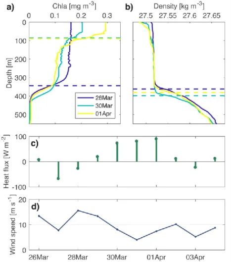
gradient between mixing and remnant layers (Fig. 1). Figure 3 illustrates how MLDbio can
207
change within 2 days in response to change in atmospheric forcing, while MLDdens remains
208
deep as a signature of the past mixing event (on March 28th). As doubling time of phytoplankton
209
cells is on the order of a day or more (Eppley et al., 1973; Goldman et al., 1979) MLDbio is not
210
likely able to capture the diurnal variability of the mixing layer. Thus, the typical timescale of 211
the MLDbio dynamics is 1-2 days. Considering the difference in timescale between MLDbio and
212
MLDdens, we do not expect to have MLDbio deeper than MLDdens except in summer stratified
213
conditions where phytoplankton can grow a few tens of meters below MLDdens, depending on
214
light penetration (see supplementary Fig. S1). Thus, MLDbio estimation > 100 m deeper than
215
MLDdens is considered as an outlier. These outliers represent only 141 profiles, or 7% of the
216
total data set. 217
218
2.4 Detection of submesoscale subduction events
219
Subduction is a 3-dimensional (3D) process involving lateral advection of water masses. Such 220
a lateral advection can be identified on a 1D profile using a state variable called spice, based on 221
anomalous temperature-salinity properties (Flament, 2002; McDougall & Krzysik, 2015; 222
Omand et al., 2015). This variable is a useful indicator of interleaving of water masses. The 223
relative standard deviation of a spice profile (RSDspice, standard deviation / mean) from 224
surface (5 m) to MLDdens is used to detect a potential intrusion of water in this layer. Application
225
of this method over the entire dataset enables to roughly identify the submesoscale subduction 226
events at a basin scale (Llort et al., 2018). 227
228
3 Results
229
3.1 Mixing versus Mixed layer dynamics
230
As proxies of the mixing and mixed layer depths, MLDbio and MLDdens, show different seasonal
231
dynamics (Fig. 4). MLDbio and MLDdens are similar in fall and early winter, when strong
232
atmospheric forcing induces turbulent mixing down to a depth that will define the upper limit 233
of the seasonal pycnocline. During these periods, temperature, salinity and phytoplankton 234
biomass are homogeneous down to MLDdens. In late winter, MLDbio and MLDdens start to
diverge. Shallower mixing layers form above remnant layers, delimited by MLDbio at the top
236
and by MLDdens at the bottom (Fig. 1). Phytoplankton in these remnant layers thus become
237
isolated from the surface layer. In summer, MLDbio is generally deeper than MLDdens and likely
238
corresponds to the lower limit of the euphotic zone. Light penetrates deeper than MLDdens and
239
allows phytoplankton growth below this layer (Fig. S1). Hence, regardless of the season, 240
MLDbio is a good indicator of the depth of the productive layer.
241 242
3.2 Impact of the mixing layer dynamics on POC export
243
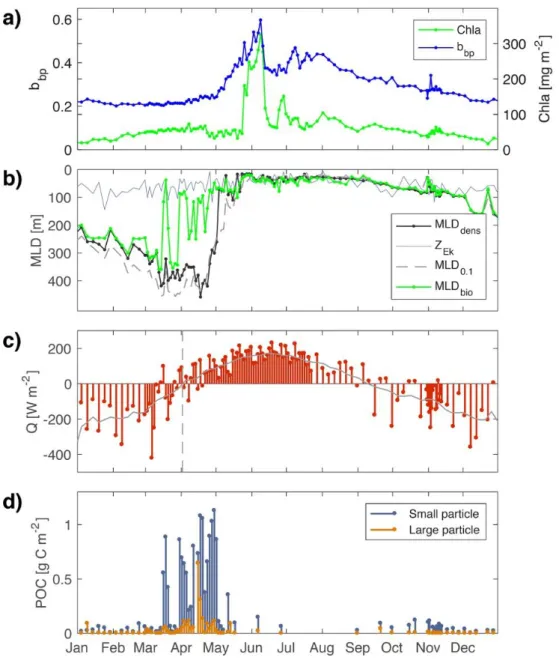
The time series of a specific float (WMO 6901516, see the float trajectory in Fig. 2) is used to 244
illustrate the impact of the mixing layer dynamics on POC export (Fig. 5). While MLDdens
245
roughly varies at the seasonal time scale, MLDbio varies at higher frequency (Fig. 5b). MLDbio
246
oscillates between MLDdens during convective mixing events (negative net heat flux, see Fig.
247
5c) and a shallower depth during stratification (positive heat flux) or shallow mixing events 248
(i.e. wind-driven mixing, see ZEk on Fig. 5b).
249
High variability of the mixing layer occurs when net heat flux (Q) oscillates around zero during 250
the winter-spring transition (March-May, Fig. 5c). The switch from negative to positive net heat 251
flux is not a rapid smooth transition. Rather, it occurs over more than a one-month period and 252
is associated with an intermittent reversal of the sign of this flux. This intermittency drives the 253
high variability of MLDbio which acts as a physical pump. Interestingly, zero-crossing net heat
254
flux, in fall, does not affect the dynamics of MLDbio which remains closely related to MLDdens.
255
The water mass history of mixing can be retraced using a single 1D profile. Indeed, MLDbio
256
marks the depth limit of recently active mixing, while MLDdens marks the depth limit of past
257
mixing. Thus, the presence of a remnant layer can be identified and used as a signature of the 258
ML pump. However, submesoscale subduction, which involves 3D processes, may also lead to 259
similar signatures (Fig. S2). Therefore, profiles with RSDspice higher than 5% were removed
260
from the analysis in order to focus exclusively on ML pump-driven mechanisms. For the 261
remaining profiles with a ML pump signature, it is assumed that each POC stock isolated in the 262
remnant layer has been exported by the ML pump. In the present study, export is defined as the 263
transfer of carbon from the turbulent productive layer to the low-turbulence remnant layer. In 264
the area sampled by float 6901516, the POC stock transferred by the ML pump is maximal 265
during the winter-spring transition when net heat fluxes switch from negative to positive values 266
(up to 1.1 g C m-2, see Fig. 5d). This maximum occurs before the main spring bloom (Fig. 5d
267
and 5a). Occasionally, the contribution of large particles or aggregates to the POC stock can be 268
significant (up to 88% during the winter-spring transition, see Fig. 5d). 269
On the basin scale, the temporal distribution of POC stocks transferred to the remnant layer 270
presents a similar pattern. POC stocks significantly increase when the sign of the smoothed heat 271
flux changes from negative to positive, with maximum values occurring 15 to 30 days later 272
(Fig. 6a), and appear to be widespread over the whole subpolar region (Fig. 6b). Note that 273
changing the RSDspice threshold from 2.5 to 10% does not impact the distribution of POC stocks
274
exported by ML pump events (see Fig. S3). 275
276
3.3 A quasi-Lagrangian approach to the ML pump
277
BGC-Argo floats are not Lagrangian floats and thus do not necessarily track coherent water 278
masses. However, depending on the temporal resolution of the floats, some successive profiles 279
may sample the same water mass, as evidenced by only subtle changes in hydrographic 280
properties. Here, within 3 pre-defined layers (surface, remnant and deep layer), we used 281
temperature, salinity and density differences of 0.1°C, 0.02 psu and 0.01 kg m-3 among
282
consecutive profiles as criteria to identify sections of float trajectories with quasi-Lagrangian 283
behaviors. We found only two sections that complied with these highly selective criteria (top 284
panels in Fig. 7a and b). The first section contains 3 profiles from float 6901516 (yellow dots 285
in Fig. 2) with 2-day intervals, and the second one contains 4 profiles from float 6901480 (green 286
dots in Fig. 2) also with 2-day intervals. The first profile of each section is well mixed up to 287
250 m depth and 600 m depth for float 6901516 and 6901480 respectively. Then, mixing stops 288
and a new mixing layer forms to a depth of around 100 m in both sections. The quasi-289
Lagrangian framework allows us to investigate the fate of Chla and bbp within these 3
pre-290
defined layers (Fig. 7). 291
In new mixing layers (i.e. surface layers), both Chla and bbp increase as a response to
292
phytoplankton growth (triangles in Fig. 7). However, the accumulation rate of Chla 293
(𝐶ℎ𝑙𝑎1 𝑑𝐶ℎ𝑙𝑎𝑑𝑡 =0.15 d-1 and 0.16 d-1) is higher than the accumulation rate of b bp (𝑏1
𝑏𝑝 𝑑𝑏𝑏𝑝
𝑑𝑡 =0.04 d
-294
1 and 0.05 d-1) for the full section period (4 days and 6 days) of float 6901516 and 6901480
295
respectively. In remnant layers, located in the twilight zone, both Chla and bbp decrease,
296
probably as a response to a change in the balance between production and heterotrophic 297
consumption (circles in Fig. 7). Like surface layers, loss rate (i.e. negative accumulation rate) 298
of Chla (0.1 d-1 and 0.06 d-1) is higher than loss rate of b
bp (0.03 d-1 and 0.005 d-1) for float
299
6901516 and 6901480 respectively. In deep layers, Chla and bbp are stable with values near zero
300
for Chla and values higher than 1x10⁻⁴ m-1 for b
bp (squares in Fig. 7). This deep bbp signal is
301
considered to be a constant background value. 302
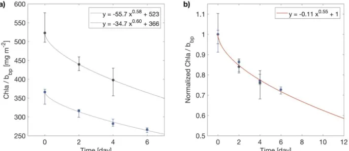
As soon as the remnant layer forms and traps particles at depth, the Chla to bbp ratio in this layer
303
starts to decrease (Fig. 8). Thus, the Chla to bbp ratio in the remnant layer can be considered as
304
a relative proxy for the freshness of the exported material. A power law function, similar to the 305
one used to calculate particle degradation in the ocean interior (Martin et al., 1987), has been 306
fitted to the data to estimate an attenuation rate. Interestingly, in the remnant layer, the 307
attenuation rate of the Chla to bbp ratio over time is similar for both floats located in different
308
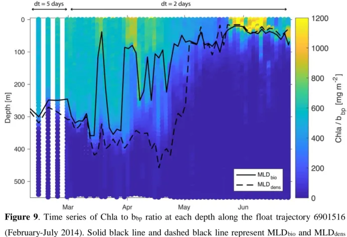
regions of the subpolar North Atlantic (similar exponent in equations of Fig. 8a). Time series 309
of Chla to bbp ratio at each depth along the float trajectories 6901516 (February-July 2014)
310
show that the ML pump export fresh material to depths ranging 0-340 m (mean 90 m) below 311
MLDbio during the whole winter-spring transition period (Fig. 9). Hence, the intermittent
312
behavior of the ML pump in the winter-spring transition generates pulses of fresh organic 313
material into the mesopelagic zone. 314
315
3.4 ML pump-driven POC flux estimates
316
We present here a method to estimate intra-seasonal ML pump-driven POC fluxes. The 317
approach consists of calculating POC fluxes over a fixed time period on a basin scale (i.e. 318
spatiotemporal binning), based on independent float profiles, i.e. without any assumption 319
regarding float Lagrangian behavior. 320
A single ML pump event is defined by three successive steps: shallow mixing at time t0 (i.e.
321
initial conditions), deep mixing at time t1 that leads to the entrainment of deep POC and
322
restratification that leads to the detrainment of POC and the formation of the remnant layer 323
observed at time t2 (Fig. S4). The net POC flux is defined as the difference between the
324
detrainment and entrainment fluxes, calculated as: 325 < 𝐸𝑒𝑛𝑡𝑟𝑎𝑖𝑛𝑚𝑒𝑛𝑡 > = < ∫ 𝑃𝑂𝐶𝑡0(𝑧) 𝑧=𝑀𝐿𝐷𝑑𝑒𝑛𝑠𝑡2 𝑧=𝑀𝐿𝐷𝑏𝑖𝑜𝑡0 𝑑𝑧 > 2 < ∆𝑡 > (1) < 𝐸𝑑𝑒𝑡𝑟𝑎𝑖𝑛𝑚𝑒𝑛𝑡 > = < 𝑃𝑂𝐶𝑡1(𝑀𝐿𝐷𝑑𝑒𝑛𝑠 𝑡2− 𝑀𝐿𝐷𝑏𝑖𝑜 𝑡2) > 2 < ∆𝑡 > (2) < 𝐸𝑛𝑒𝑡 > = < 𝐸𝑑𝑒𝑡𝑟𝑎𝑖𝑛𝑚𝑒𝑛𝑡 > − < 𝐸𝑒𝑛𝑡𝑟𝑎𝑖𝑛𝑚𝑒𝑛𝑡 > (3) The numerator of equation 1 stands for the POC entrained by the deep mixing event at time t1
326
while the numerator of equation 2 stands for the POC detrained during the restratification event 327
(Fig. S5). 𝑀𝐿𝐷𝑑𝑒𝑛𝑠 𝑡2marks the depth limit of the deep mixing event and (𝑀𝐿𝐷𝑑𝑒𝑛𝑠 𝑡2 − 328
𝑀𝐿𝐷𝑏𝑖𝑜 𝑡2) represents the thickness of the remnant layer observed at time t2. 𝑃𝑂𝐶𝑡1, the POC
329
concentration within the deep mixing layer at time t1, is estimated as the mean 𝑃𝑂𝐶𝑡0 from the
330
surface to 𝑀𝐿𝐷𝑑𝑒𝑛𝑠 𝑡2(Fig. S5). Brackets indicate spatiotemporal binning. ∆𝑡 is the time elapsed 331
between the observation at time t2 and the last mixing event at time t1, and can be derived from
332
the best-fit power law function in Fig. 8b as: 333 ∆𝑡 = 𝑡2− 𝑡1 = ( 𝐶ℎ𝑙𝑎 𝑏⁄ 𝑏𝑝 𝑡2−𝐶ℎ𝑙𝑎 𝑏⁄ 𝑏𝑝 𝑡1 −0.11 𝐶ℎ𝑙𝑎 𝑏⁄ 𝑏𝑝 𝑡1 ) 1 0.55 (4) where 𝐶ℎ𝑙𝑎 𝑏⁄ 𝑏𝑝
𝑡2 is the ratio of the median Chla to the median bbp within the remnant layer
334
and 𝐶ℎ𝑙𝑎 𝑏⁄ 𝑏𝑝
𝑡1 is the ratio within the deep mixing layer at time t1. 𝐶ℎ𝑙𝑎 𝑏⁄ 𝑏𝑝 𝑡1is estimated
335
the same way as 𝑃𝑂𝐶𝑡1, by averaging 𝐶ℎ𝑙𝑎𝑡0 and 𝑏𝑏𝑝𝑡0 from the surface to 𝑀𝐿𝐷𝑑𝑒𝑛𝑠 𝑡2. While
336
𝐶ℎ𝑙𝑎 𝑏⁄ 𝑏𝑝
𝑡2, 𝑀𝐿𝐷𝑑𝑒𝑛𝑠 𝑡2, and 𝑀𝐿𝐷𝑏𝑖𝑜 𝑡2 are measured at time t2 when a remnant layer is
337
identified (i.e. ML pump signature), initial conditions prevailing at time t0 (i.e.
338
𝑀𝐿𝐷𝑏𝑖𝑜𝑡0, 𝑃𝑂𝐶𝑡0, 𝐶ℎ𝑙𝑎𝑡0, 𝑏𝑏𝑝𝑡
0), from which variable at time t1 are derived, are unknown. In
339
order to provide a set of potential initial conditions for each profile with a ML pump signature, 340
all available profiles, from 2014 to 2016, within a radius of 300 km and a time period of 15 341
days (all years included), are collected (Fig. S6). To keep only realistic initial conditions, three 342
requisites are needed: 1) 𝐶ℎ𝑙𝑎 𝑏⁄ 𝑏𝑝
𝑡1, derived from 𝐶ℎ𝑙𝑎𝑡0 and 𝑏𝑏𝑝𝑡0, is higher than
343
𝐶ℎ𝑙𝑎 𝑏⁄ 𝑏𝑝
𝑡, 2) 𝑀𝐿𝐷𝑏𝑖𝑜𝑡0 is shallower than 𝑀𝐿𝐷𝑑𝑒𝑛𝑠 𝑡2, 3) ∆𝑡 is less than 20 days. The choice
344
of a threshold of 20 days is based on the basin-scale analysis of the density function of 345
𝐶ℎ𝑙𝑎 𝑏⁄ 𝑏𝑝 both within the mixing and remnant layers (Fig. S7). Using the attenuation rate of
346
𝐶ℎ𝑙𝑎 𝑏⁄ 𝑏𝑝 shown in Fig. 8b, we modeled the cumulative density function within the remnant 347
layer for ∆𝑡 ranging from 1 to 5, 20 or 35 days (see caption of Fig. S7) and compared it with 348
the measured cumulative density function. The cumulative density function for ∆t ranging from 349
1 to 20 days is the one which best fit the measured density function within the remnant layer. 350
Therefore, a threshold of 20 days seems appropriate to reject unrealistic initial conditions. All 351
the initial conditions that complied with these 3 requisites are used to calculate a mean ∆𝑡 and 352
associated standard deviation for each profile presenting a ML pump signature. Over a fixed 353
time period, the mean duration of ML pump events is estimated as 2 < ∆𝑡 > (Fig. S8). Indeed, 354
as the profiling time t2 is random between the last mixing event at time t1 and the next one,
potentially at t3, ∆𝑡 should range from 0 to (𝑡3 − 𝑡1), with mean value < ∆𝑡 > = (𝑡3− 𝑡1)/2.
356
Here, a time period of 10 days is used, with a minimum of 6 profiles as an additional 357
requirement to correctly estimate the mean duration of ML pump events. 358
Figure 10 presents estimates of entrainment, detrainment and net POC fluxes averaged over 10-359
day periods in the whole subpolar North Atlantic Ocean. As expected, the temporal pattern in 360
detrainment fluxes (Fig. 10c) is similar to the one observed in POC stock in the remnant layer 361
(Fig. 6a) and the one in detrained POC stocks estimated from initial conditions (Fig. 10a, 362
numerators in equation 2, blue color). Maximum detrainment fluxes and net export fluxes (125 363
and 55 mg C m-2 d-1, respectively) both occur few days after the switch in the sign of the heat
364
flux. Approximately 40 days later, detrainment fluxes decrease by a factor of 2 to 3 and net 365
POC fluxes are reduced to near zero. The length of error bars represents the average standard 366
deviation of initial conditions associated to each ML pump signature detected within a 10-day 367
time period. Note that fluxes were not estimated between days 70 to 90 because the number of 368
profiles presenting a ML pump signature was below the critical threshold of 6 profiles (Fig. 369 S8). 370 371 4 Discussion 372
4.1 Mixing versus mixed layer depth
373
Observations of vertical profiles of density and Chla in late winter and spring (Fig. 4) suggest 374
that density-derived methods to estimate MLD have to be interpreted with caution when 375
considering controls on phytoplankton processes. A simple comparison (linear correlation 376
analysis, Fig. S9) between MLDbio and MLD estimated with different density-difference criteria
377
revealed that most of these criteria do not detect subtle changes in density, which affect the 378
phytoplankton vertical distribution (Lacour et al., 2017). As a consequence, studies estimating 379
depth-integrated Chla by multiplying the concentration of surface Chla (measured by satellite) 380
by the depth of a density-derived mixed layer could overestimate the Chla stock, especially 381
during the winter to spring transition. Indeed, the widely used density difference criteria of 0.1 382
kg m-3 leads, in the present study, to a mean overestimation of 46% of the spring phytoplankton
383
stock (comparison of the real stock measured by the float in the mixed layer with the estimated 384
stock based on surface Chla). However, a density criterion of 0.01 kg m-3, which shows the best
385
correlation with MLDbio, leads to a mean overestimation of only 3%. Most density difference
386
thresholds are not suited to capture the intra-seasonal dynamics of the mixing layer which 387
affects the vertical distribution of phytoplankton biomass. 388
4.2 The ML pump signature
390
The ML pump is a complex mechanism which can occur on a variety of timescales, from diurnal 391
to seasonal scales. Observing this mechanism at specific scales requires appropriate approaches. 392
Combining Argo float data with satellite estimates of POC, Dall’Olmo et al. (2016) provided 393
first estimates of the carbon flux induced by the seasonal ML pump at global scale. The rate of 394
change of the MLD at a time interval of 10 days along Argo float trajectories was exploited. 395
Therefore, the high-frequency variability (< 10 days) was not considered and assumption of 396
spatial homogeneity was required. This approach revealed the importance of the ML pump in 397
seasonal carbon fluxes but the episodic nature of carbon export was not considered. The 398
innovative approach, here, is to use a single profile to retrace the water mass history of mixing 399
and thus relax the assumption of spatial homogeneity. Using MLDbio as the depth limit of a
400
recent mixing and MLDdens as the depth limit of a past mixing, the presence of a remnant layer
401
can be identified and used as a signature of the ML pump. Although the typical timescale of 402
MLDbio is known (~1-2 days), the timescale of MLDdens is more difficult to assess. Figure 3b
403
shows that MLDdens is still deep 4 days after deep convection stopped and figure 5b reveals a
404
~10-day delay between the permanent shoaling of MLDbio around 100 m and the shoaling of
405
MLDdens. It is thus assumed that MLDdens roughly corresponds to a mixed layer on a 10-day
406
timescale. Thereby, the signature of ML pump likely reveals recent export of organic matter 407
thus allowing the assessment of the episodic nature of this mechanism. Although this approach 408
allows exploration of the intra-seasonal dynamics of the ML pump, the diurnal timescales are 409
not assessed. 410
The strongest signatures of the ML pump (i.e. maximum POC stock in the remnant layer) were 411
recorded when the net heat flux switches from negative to positive values in early spring. 412
Interestingly, the switch from positive to negative values in fall did not affect MLDbio which
413
remained closely related to MLDdens (Fig. 5). This dissymmetry was likely due to the
414
mechanical effect of wind, that mixes the upper layer (Woods, 1980). The Ekman length scale, 415
which is the dominant mixing length scale when heat fluxes are small (Brody & Lozier, 2014), 416
indicated that mixing reached depths as deep as MLDdens at this time of the year (Fig. 5b).
417
Phytoplankton can be redistributed within MLDdens even if net heat fluxes become positive,
418
thus inhibiting the formation of remnant layers. 419
Warming of the upper layer is not the only source of stratification. In addition to freshwater 420
flux, 3D processes involving lateral advection are known to quickly restratify deep mixed layers 421
(Brainerd & Gregg, 1993; Hosegood et al., 2006, 2008; Johnson et al., 2016). Submesoscale 422
eddies or Ekman buoyancy flux can slump horizontal density gradient to create vertical 423
stratification (Boccaletti et al., 2007; Thomas & Lee, 2005). These processes, which generate a 424
signature similar to the ML pump, are often associated with submesoscale subduction (Omand 425
et al., 2015). Based on a RSDspice threshold of 5%, it can be estimated that almost 40% of the
426
profiles displaying a ML pump signature were affected by lateral water intrusion. As mentioned 427
by Ho and Marra (1994), quantifying ML pump export is difficult since local and advective 428
effects have to be distinguished. Here, a RSDspice threshold of 5% appeared adequate to identify
429
and subsequently remove profiles affected by advective effects. However, it is worth noting 430
that lateral restratifications could contribute to the export through the ML pump. Indeed, lateral 431
restratification can stimulate phytoplankton production (Mahadevan et al., 2012), even during 432
winter (Lacour et al., 2017), and the resulting biomass could be exported later, following a deep 433
mixing event. Although this study focuses on 1D processes, lateral restratification may also 434
stimulate the ML pump export, especially in winter when positive heat flux events are scarcer. 435
436
4.3 Fate of Chla and bbp signal in the remnant layer
437
Quasi-Lagrangian sections of float trajectories allowed us to investigate the fate of Chla and bbp
438
signals in surface and remnant layers after a stratification event (Fig. 7). Chla signals increased 439
faster in the surface layer and decreased faster in the remnant layer than the bbp signals. The
440
main reason for this discrepancy rests on the nature of the particles contributing to both Chla 441
and bbp signal. While phytoplankton cells contribute nearly all of the Chla signal (colored
442
dissolve organic matter may also contribute slightly to the Chla signal; Xing et al., 2017), 443
bacteria, protists, detritus and mineral material also contribute to the bbp signal
(Martinez-444
Vicente et al., 2012; Stramski et al., 1991, 2001, 2004). Therefore, in the surface layer, an 445
increase in phytoplankton production does not lead to a similar relative increase in the Chla and 446
bbp signals. In addition, taxonomic changes in the phytoplankton community could further
447
increase the Chla signal relative to the bbp signal. Indeed, the local restratification could enhance
448
the light environment and stimulate larger phytoplankton, such as diatoms, with higher Chla to 449
bbp ratio (Cetinić et al., 2015; Lacour et al., 2017; Rembauville et al., 2017). In the twilight
450
remnant layer, change in the balance between production and consumption leads to a decrease 451
in both Chla and bbp. However, the faster decrease in the Chla signal may be explained by
452
multiple factors. First, fresh phytoplankton (i.e. Chla signal) are possibly preferentially 453
consumed compared to detritus and other material contributing to the bbp signal. Second, the
454
consumption of phytoplankton cells could enhance the growth of heterotrophic organisms such 455
as bacteria or protists which would also contribute to the bbp signal. Third, physical and
456
biological disaggregation of large particles at depth (Alldredge et al., 1990; Burd & Jackson, 457
2009; Cho & Azam, 1988) may enhance the bbp signal, which likely corresponds to small
458
particles (0.2-20 µm; Dall’Olmo & Mork, 2014), and counteract the decrease in bbp due to
459
consumption. Finally, additional decrease in Chla could be attributed to physiological 460
adaptations to darkness which involve a reduced fluorescence per unit of Chla (Murphy & 461
Cowles, 1997). 462
463
4.4 Towards global event-based POC flux estimates
464
Present carbon flux estimates are mainly based on a limited number of observations at specific 465
times and locations. Scaling up these observations to obtain regional and global estimates may 466
neglect or underestimate the contribution of episodic events, leading to our inability to balance 467
biogeochemical budgets in the mesopelagic (Burd et al., 2016). The ML pump is a typical 468
mechanism driving episodic export of organic carbon to depth. Based on high-resolution 469
observations from a dense BGC-Argo float network, we assessed for the first time the intra-470
seasonal dynamics of ML pump-driven POC fluxes on a basin scale (Fig. 10). This approach 471
required three main assumptions: 472
(1) We assumed that initial conditions (i.e. Chla b⁄ bp
t0, POCMLDbio t0) prevailing before a
473
ML pump event can be predicted from a “climatology” of profiles collected in the area 474
of the event location. Three selection criteria (see section 3.4) have been applied to 475
ensure that only realistic initial conditions have been used. Error bars in figure 10a and 476
b show that the variability related to these initial conditions remains reasonably small. 477
(2) We assumed that the mean duration of ML pump events is twice the mean time < ∆t > 478
between the observation of the ML pump signature and the last mixing event. An 479
analysis of ML pump events recorded by a Lagrangian float revealed that the absolute 480
error related to this assumption is less than 0.2 days as long as the number of events 481
averaged is more than 6 (Fig. S6). As the BGC-Argo dataset will expand in the future, 482
we will be able to reduce the spatiotemporal binning with the goal of quantifying event-483
based POC fluxes on a basin scale. 484
(3) The attenuation rate of the Chla to bbp ratio in the remnant layer is assumed to be
485
constant on a basin scale. The present analysis demonstrated that this attenuation rate is 486
similar within two different regions of the subpolar North Atlantic. However, additional 487
measurements in remnant layers are clearly needed to better constrain the attenuation 488
rate of the Chla to bbp ratio and reduce uncertainties associated to this approach. More
489
generally, further investigations on particle composition, microbial metabolism and 490
transformation processes occurring in remnant layers are required to better understand 491
the fate of the organic material exported by the ML pump. 492
The mean ML pump-driven net POC flux peaks at 55 mg C m-2 d-1 in late winter and drops
493
down to negative values when the water column stabilizes in summer. During this period, the 494
entrainment flux due to wind-driven mixing events can exceed the detrainment flux, as the light 495
penetration allows phytoplankton to grow below the mixing layer. The net amount of POC 496
exported during the winter-spring transition (i.e. positive net export) is the fraction of fresh 497
organic material that we expect to be consumed in the mesopelagic. Therefore, the intra-498
seasonal ML pump may sustain the mesopelagic ecosystem before the spring bloom period. 499
500
4.5 Role of the ML pump in sustaining mesopelagic ecosystems
501
The recurrence of widespread ML pump events during a relatively large time period (> 90 days) 502
implies that this mechanism may be of great significance in supplying the energy required by 503
the mesopelagic heterotrophic community (Dall’Olmo et al., 2016). The particles mixed 504
downward through the ML pump are rich in fresh phytoplankton and detritus, so potentially of 505
high nutritional content for grazers located below the mixing layer (Steinberg & Landry, 2017). 506
Export of both small and large particles to the mesopelagic region suggests that this mechanism 507
could sustain zooplankton populations with different feeding preferences (Fenchel, 1980; 508
Irigoien et al., 2000; Turner et al., 2001; Turner, 2004). Products from zooplankton activities 509
would then sustained microbial populations and higher trophic levels (Steinberg & Landry, 510
2017). Therefore, the ML pump could supply a major source of energy to the whole 511
mesopelagic ecosystem during the winter to spring transition. 512
Many studies reported that the bulk of zooplankton populations resides just below the turbulent 513
mixing layer (Incze et al., 2001; Lagadeuc et al., 1997; Mackas et al., 1993). The turbulence-514
avoidance behavior of grazers has been invoked to explain their vertical distribution in the water 515
column (Franks, 2001). However, the reason for this behavior is not clear. Turbulence is known 516
to influence encounter and ingestion rate of zooplankton and larger predators, but both positive 517
and negative effects have been reported (MacKenzie, 2000). During the winter to spring 518
transition, the vertical distribution of grazers could be a direct consequence of the ML pump. 519
These organisms could swim deep during turbulent mixing events, then immediately return to 520
the remnant layer upon restratification to take advantage of fresh food supplied by the ML 521
pump. For this reason, export is defined here as a transfer from the turbulent productive layer 522
to the remnant non-productive layer. 523
Finally, the ML pump during the winter-spring transition could trigger the seasonal 524
development of overwintering organisms such as copepods so that their reproduction would 525
coincide with the forthcoming spring bloom (Bishop & Wood, 2009). We can thus speculate 526
that the frequency of episodic ML pump export events during the pre-bloom period may 527
modulate the timing of the maturation phase of copepods and indirectly impact the magnitude 528
of the spring bloom. 529
530
5 Conclusion
531
The density of the BGC-Argo float network has enabled, for the first time, investigation of the 532
intra-seasonal dynamics of the ML pump on a basin scale. ML pump signatures are widespread 533
over the subpolar North Atlantic Ocean and span a large temporal window preceding the spring 534
bloom. To date, the high-frequency dynamics of bio-physical mechanisms had clearly been 535
overlooked due to the lack of well-suited observational tools. Yet, ML pump episodic events 536
may contribute significantly to the export of fresh organic matter during the late winter and 537
early spring periods. This mechanism may sustain the development of overwintering organisms 538
such as copepods with potential impact on the characteristics of the forthcoming spring 539
phytoplankton bloom through predator-prey interactions. Further investigations of episodic 540
events will undoubtedly provide new insights on life strategies and food web interactions, and 541
potentially address the fundamental limitations of assuming steady-state conditions. 542
543
Acknowledgments
544
This work represents a contribution to the REMOCEAN project (REMotely sensed 545
biogeochemical cycles in the OCEAN, GA 246777) funded by the European Research Council 546
and the ATLANTOS EU project (grant agreement 2014-633211) funded by H2020 program. 547
BGC-Argo data are publicly available at ftp://ftp.ifremer.fr/ifremer/argo/dac/coriolis/. We 548
thank C. Schmechtig and A. Poteau for BGC-Argo float data management and M. Gali for 549 fruitful discussions. 550 551 References 552
Alldredge, A. L., Granata, T. C., Gotschalk, C. C., & Dickey, T. D. (1990). The physical 553
strength of marine snow and its implications for particle disaggregation in the ocean. 554
Limnology and Oceanography, 35(7), 1415–1428.
555
https://doi.org/10.4319/lo.1990.35.7.1415 556
Barth, J. A., Cowles, T. J., Kosro, P. M., Shearman, R. K., Huyer, A., & Smith, R. L. (2002). 557
Injection of carbon from the shelf to offshore beneath the euphotic zone in the California 558
Current. Journal of Geophysical Research, 107(C6), 3057. 559
https://doi.org/10.1029/2001JC000956 560
Bishop, J. K. B., Conte, M. H., Wiebe, P. H., Roman, M. R., & Langdon, C. (1986). 561
Particulate matter production and consumption in deep mixed layers: observations in a 562
warm-core ring. Deep Sea Research Part A. Oceanographic Research Papers, 33(11– 563
12), 1813–1841. https://doi.org/10.1016/0198-0149(86)90081-6 564
Bishop, J. K. B., & Wood, T. J. (2009). Year-round observations of carbon biomass and flux 565
variability in the Southern Ocean. Global Biogeochemical Cycles, 23(2), n/a-n/a. 566
https://doi.org/10.1029/2008GB003206 567
Boccaletti, G., Ferrari, R., & Fox-Kemper, B. (2007). Mixed Layer Instabilities and 568
Restratification. Journal of Physical Oceanography, 37(9), 2228–2250. 569
https://doi.org/10.1175/JPO3101.1 570
Boss, E., & Behrenfeld, M. (2010). In situ evaluation of the initiation of the North Atlantic 571
phytoplankton bloom. Geophysical Research Letters, 37(18). 572
https://doi.org/10.1029/2010GL044174 573
Brainerd, K. E., & Gregg, M. C. (1993). Diurnal restratification and turbulence in the oceanic 574
surface mixed layer: 1. Observations. Journal of Geophysical Research, 98(C12), 22645. 575
https://doi.org/10.1029/93JC02297 576
Brainerd, K. E., & Gregg, M. C. (1995). Surface mixed and mixing layer depths. Deep-Sea 577
Research Part I, 42(9), 1521–1543. https://doi.org/10.1016/0967-0637(95)00068-H
578
Briggs, N., Perry, M. J., Cetinić, I., Lee, C., D’Asaro, E., Gray, A. M., & Rehm, E. (2011). 579
High-resolution observations of aggregate flux during a sub-polar North Atlantic spring 580
bloom. Deep Sea Research Part I: Oceanographic Research Papers, 58(10), 1031–1039. 581
https://doi.org/10.1016/j.dsr.2011.07.007 582
Brody, S. R., & Lozier, M. S. (2014). Changes in dominant mixing length scales as a driver of 583
subpolar phytoplankton bloom initiation in the North Atlantic. Geophysical Research 584
Letters, 41(9), 3197–3203. https://doi.org/10.1002/2014GL059707
585
Buesseler, K. O., & Boyd, P. W. (2009). Shedding light on processes that control particle 586
export and flux attenuation in the twilight zone of the open ocean. Limnology and 587
Oceanography, 54(4), 1210–1232. https://doi.org/10.4319/lo.2009.54.4.1210
588
Burd, A. B., Hansell, D. A., Steinberg, D. K., Anderson, T. R., Arístegui, J., Baltar, F., … 589
Tanaka, T. (2010). Assessing the apparent imbalance between geochemical and 590
biochemical indicators of meso- and bathypelagic biological activity: What the @$#! is 591
wrong with present calculations of carbon budgets? Deep-Sea Research Part II: Topical 592
Studies in Oceanography, 57(16), 1557–1571. https://doi.org/10.1016/j.dsr2.2010.02.022
593
Burd, A. B., & Jackson, G. A. (2009). Particle Aggregation. Annual Review of Marine 594
Science, 1(1), 65–90. https://doi.org/10.1146/annurev.marine.010908.163904
595
Burd, A., Buchan, A., Church, M., Landry, M., McDonnell, A., Passow, U., … Benway, H. 596
(2016). Towards a transformative understanding of the ocean ’ s biological pump : 597
Priorities for future research. Report of the NSF Biology of the Biological Pump
598
Workshop, February 19-20, 2016. Woods Hole, MA: Ocean Carbon and
599
Biogeochemistry (OCB) Program. https://doi.org/10.1575/1912/8263 600
Carlson, C. A., Ducklow, H. W., & Michaels, A. F. (1994). Annual flux of dissolved organic 601
carbon from the euphotic zone in the northwestern Sargasso Sea. Nature, 371(6496), 602
405–408. https://doi.org/10.1038/371405a0 603
Cetinić, I., Perry, M. J., Briggs, N. T., Kallin, E., D’Asaro, E. a., & Lee, C. M. (2012). 604
Particulate organic carbon and inherent optical properties during 2008 North Atlantic 605
Bloom Experiment. Journal of Geophysical Research, 117(C6), C06028. 606
https://doi.org/10.1029/2011JC007771 607
Cetinić, I., Perry, M. J., D’Asaro, E., Briggs, N., Poulton, N., Sieracki, M. E., & Lee, C. M. 608
(2015). A simple optical index shows spatial and temporal heterogeneity in 609
phytoplankton community composition during the 2008 North Atlantic Bloom 610
Experiment. Biogeosciences, 12(7), 2179–2194. https://doi.org/10.5194/bg-12-2179-611
2015 612
Cho, B. C., & Azam, F. (1988). Major role of bacteria in biogeochemical fluxes in the ocean’s 613
interior. Nature. https://doi.org/10.1038/332441a0 614
Dall’Olmo, G., Dingle, J., Polimene, L., Brewin, R. J. W., & Claustre, H. (2016). Substantial 615
energy input to the mesopelagic ecosystem from the seasonal mixed-layer pump. Nature 616
Geoscience. https://doi.org/10.1038/ngeo2818
617
Dall’Olmo, G., & Mork, K. A. (2014). Carbon export by small particles in the Norwegian 618
Sea. Geophysical Research Letters, 41(8), 2921–2927. 619
https://doi.org/10.1002/2014GL059244 620
Ducklow, H., Steinberg, D., & Buesseler, K. (2001). Upper Ocean Carbon Export and the 621
Biological Pump. Oceanography, 14(4), 50–58. https://doi.org/10.5670/oceanog.2001.06 622
Eppley, R. W., Renger, E. H., Venrick, E. L., Mullin, M. M., & Jul, N. (1973). A Study of 623
Plankton Dynamics and Nutrient Cycling in the Central Gyre of the North Pacific Ocean. 624
Limnology and Oceanography, 18(4), 534–551.
625
https://doi.org/10.4319/lo.1973.18.4.0534 626
Fenchel, T. (1980). Suspension feeding in ciliated protozoa: Functional response and particle 627
size selection. Microbial Ecology, 6(1), 1–11. https://doi.org/10.1007/BF02020370 628
Franks, P. J. S. (2001). Turbulence avoidance: An alternate explanation of turbulence-629
enhanced ingestion rates in the field. Limnology and Oceanography, 46(4), 959–963. 630
https://doi.org/10.4319/lo.2001.46.4.0959 631
Gardner, W. D., Chung, S. P., Richardson, M. J., & Walsh, I. D. (1995). The oceanic mixed-632
layer pump. Deep Sea Research Part II: Topical Studies in Oceanography, 42(2–3), 633
757–775. https://doi.org/10.1016/0967-0645(95)00037-Q 634
Garside, C., & Garside, J. C. (1993). The “f-ratio” on 20°W during the North Atlantic Bloom 635
Experiment. Deep-Sea Research Part II, 40(1–2), 75–90. https://doi.org/10.1016/0967-636
0645(93)90007-A 637
Giering, S. L. C., Sanders, R., Lampitt, R. S., Anderson, T. R., Tamburini, C., Boutrif, M., … 638
Mayor, D. J. (2014). Reconciliation of the carbon budget in the ocean’s twilight zone. 639
Nature, 507(7493), 480–483. https://doi.org/10.1038/nature13123
640
Giering, S. L. C., Sanders, R., Martin, A. P., Lindemann, C., Möller, K. O., Daniels, C. J., … 641
St. John, M. A. (2016). High export via small particles before the onset of the North 642
Atlantic spring bloom. Journal of Geophysical Research: Oceans, 121(9), 6929–6945. 643
https://doi.org/10.1002/2016JC012048 644
Goldman, J. C., McCarthy, J. J., & Peavey, D. G. (1979). Growth rate influence on the 645
chemical composition of phytoplankton in oceanic waters. Nature, 279(5710), 210–215. 646
https://doi.org/10.1038/279210a0 647
Ho, C., & Marra, J. (1994). Early-spring export of phytoplankton production in the northeast 648
Atlantic Ocean. Marine Ecology Progress Series, 114(1), 197–202. 649
https://doi.org/10.3354/meps114197 650
Hosegood, P., Gregg, M. C., & Alford, M. H. (2006). Sub-mesoscale lateral density structure 651
in the oceanic surface mixed layer. Geophysical Research Letters, 33(22), L22604. 652
https://doi.org/10.1029/2006GL026797 653
Hosegood, P. J., Gregg, M. C., & Alford, M. H. (2008). Restratification of the Surface Mixed 654
Layer with Submesoscale Lateral Density Gradients: Diagnosing the Importance of the 655
Horizontal Dimension. Journal of Physical Oceanography, 38(11), 2438–2460. 656
https://doi.org/10.1175/2008JPO3843.1 657
Huisman, J., Oostveen, P. van, & Weissing, F. J. (1999). Critical Depth and Critical 658
Turbulence: Two Different Mechanisms for the Development of Phytoplankton Blooms. 659
Limnology and Oceanography, 44(7), 1781–1787. Retrieved from
660
http://www.jstor.org/stable/2670414 661
Incze, L., Hebert, D., Wolff, N., Oakey, N., & Dye, D. (2001). Changes in copepod 662
distributions associated with increased turbulence from wind stress. Marine Ecology 663
Progress Series, 213, 229–240. https://doi.org/10.3354/meps213229
664
Irigoien, X., Harris, R. P., Head, R. N., & Harbour, D. (2000). The influence of diatom 665
abundance on the egg production rate of Calanus helgolandicus in the English Channel. 666
Limnology and Oceanography, 45(6), 1433–1439.
667
https://doi.org/10.4319/lo.2000.45.6.1433 668
Johnson, L., Lee, C. M., & D’Asaro, E. A. (2016). Global Estimates of Lateral Springtime 669
Restratification. Journal of Physical Oceanography, 46(5), 1555–1573. 670
https://doi.org/10.1175/JPO-D-15-0163.1 671
Jónasdóttir, S. H., Visser, A. W., Richardson, K., & Heath, M. R. (2015). Seasonal copepod 672
lipid pump promotes carbon sequestration in the deep North Atlantic. Proceedings of the 673
National Academy of Sciences, 112(39), 12122–12126.
674
https://doi.org/10.1073/pnas.1512110112 675
Koeve, W., Pollehne, F., Oschlies, A., & Zeitzschel, B. (2002). Storm-induced convective 676
export of organic matter during spring in the northeast Atlantic Ocean. Deep-Sea 677
Research Part I: Oceanographic Research Papers, 49(8), 1431–1444.
678
https://doi.org/10.1016/S0967-0637(02)00022-5 679
Kwon, E. Y., Primeau, F., & Sarmiento, J. L. (2009). The impact of remineralization depth on 680
the air-sea carbon balance. Nature Geoscience, 2(9), 630–635. 681
https://doi.org/10.1038/ngeo612 682
Lacour, L., Ardyna, M., Stec, K. F., Claustre, H., Prieur, L., Poteau, A., … Iudicone, D. 683
(2017). Unexpected winter phytoplankton blooms in the North Atlantic subpolar gyre. 684
Nature Geoscience, 10(11), 836–839. https://doi.org/10.1038/NGEO3035
685
Lagadeuc, Y., Boulé, M., & Dodson, J. J. (1997). Effect of vertical mixing on the vertical 686
distribution of copepods in coastal waters. Journal of Plankton Research, 19(9), 1183– 687
1204. https://doi.org/10.1093/plankt/19.9.1183 688
Lampitt, R. S., Salter, I., de Cuevas, B. A., Hartman, S., Larkin, K. E., & Pebody, C. A. 689
(2010). Long-term variability of downward particle flux in the deep northeast Atlantic: 690
Causes and trends. Deep-Sea Research Part II: Topical Studies in Oceanography, 691
57(15), 1346–1361. https://doi.org/10.1016/j.dsr2.2010.01.011
692
Lévy, M., Klein, P., & Treguier, A.-M. (2001). Impact of sub-mesoscale physics on 693
production and subduction of phytoplankton in an oligotrophic regime. Journal of 694
Marine Research, 59(4), 535–565. https://doi.org/10.1357/002224001762842181
695
Llort, J., Langlais, C., Matear, R., Moreau, S., Lenton, A., & Strutton, P. G. (2018). 696
Evaluating Southern Ocean Carbon Eddy-Pump From Biogeochemical-Argo Floats. 697
Journal of Geophysical Research: Oceans, 123(2), 971–984.
698
https://doi.org/10.1002/2017JC012861 699
Mackas, D. L., Sefton, H., Miller, C. B., & Raich, A. (1993). Vertical habitat partitioning by 700
large calanoid copepods in the oceanic subarctic Pacific during Spring. Progress in 701
Oceanography, 32(1), 259–294. https://doi.org/10.1016/0079-6611(93)90017-8
702
MacKenzie, B. R. (2000). Turbulence, larval fish ecology and fisheries recruitment: a review 703
of field studies. Oceanologica Acta, 23(4), 357–375. https://doi.org/10.1016/S0399-704
1784(00)00142-0 705
Mahadevan, a., D’Asaro, E., Lee, C., & Perry, M. J. (2012). Eddy-Driven Stratification 706
Initiates North Atlantic Spring Phytoplankton Blooms. Science, 337(6090), 54–58. 707
https://doi.org/10.1126/science.1218740 708
Martin, J. H., Knauer, G. A., Karl, D. M., & Broenkow, W. W. (1987). VERTEX: carbon 709