Effects of energetic electrons on the electrodynamics in the ionosphere

HAL Id: hal-00317232

https://hal.archives-ouvertes.fr/hal-00317232

Submitted on 1 Jan 2004

HAL is a multi-disciplinary open access

archive for the deposit and dissemination of

sci-entific research documents, whether they are

pub-lished or not. The documents may come from

teaching and research institutions in France or

abroad, or from public or private research centers.

L’archive ouverte pluridisciplinaire HAL, est

destinée au dépôt et à la diffusion de documents

scientifiques de niveau recherche, publiés ou non,

émanant des établissements d’enseignement et de

recherche français ou étrangers, des laboratoires

publics ou privés.

the ionosphere

A. Aksnes, J. Stadsnes, G. Lu, N. Østgaard, R. R. Vondrak, D. L. Detrick, T.

J. Rosenberg, G. A. Germany, M Schulz

To cite this version:

A. Aksnes, J. Stadsnes, G. Lu, N. Østgaard, R. R. Vondrak, et al.. Effects of energetic electrons on

the electrodynamics in the ionosphere. Annales Geophysicae, European Geosciences Union, 2004, 22

(2), pp.475-496. �hal-00317232�

Effects of energetic electrons on the electrodynamics in the

ionosphere

A. Aksnes1, J. Stadsnes1, G. Lu2, N. Østgaard3, R. R. Vondrak4, D. L. Detrick5, T. J. Rosenberg5, G. A. Germany6, and M. Schulz7

1_{Department of Physics, University of Bergen, Bergen, Norway}

2_{High Altitude Observatory/National Center of Atmospheric Research, 3450 Mitchell Lane, Boulder, CO 80301, USA} 3_{University of California, Berkeley, CA 94720-7450, USA}

4_{NASA/Goddard Space Flight Center, Greenbelt, MD 20771, USA} 5_{University of Maryland, College Park, MD 20742, USA}

6_{University of Alabama in Huntsville, AL 35899, USA}

7_{Lockheed Martin Advanced Technology Center, 3251 Hanover Street, Palo Alto, CA 94304, USA}

Received: 21 March 2003 – Revised: 13 June 2003 – Accepted: 2 July 2003 – Published: 1 January 2004

Abstract. From the observations by the PIXIE and UVI cameras on board the Polar satellite, we derive global maps of the precipitating electron energy spectra from less than 1 keV to 100 keV. Based on the electron spectra, we gen-erate instantaneous global maps of Hall and Pedersen con-ductances. The UVI camera provides good coverage of the lower electron energies contributing most to the Pedersen conductance, while PIXIE captures the high energy compo-nent of the precipitating electrons affecting the Hall conduc-tance. By characterizing the energetic electrons from some tens of keV and up to about 100 keV using PIXIE X-ray mea-surements, we will, in most cases, calculate a larger electron flux at higher energies than estimated from a simple extrap-olation of derived electron spectra from UVI alone. Instan-taneous global conductance maps derived with and without inclusion of PIXIE data have been implemented in the As-similative Mapping of Ionospheric Electrodynamics (AMIE) procedure, to study the effects of energetic electrons on elec-trodynamical parameters in the ionosphere. We find that the improved electron spectral characterization using PIXIE data most often results in a larger Hall conductance and a smaller inferred electric field. In some localized regions the increase in the Hall conductance can exceed 100%. On the contrary, the Pedersen conductance remains more or less unaffected by the inclusion of the PIXIE data. The calculated polar cap potential drop may decrease more than 10%, resulting in a reduction of the estimated Joule heating integrated over the Northern Hemisphere by up to 20%. Locally, Joule heat-ing may decrease more than 50% in some regions. We also find that the calculated energy flux by precipitating electrons increases around 5% when including the PIXIE data. Com-bined with the reduction of Joule heating, this results in a decrease in the ratio between Joule heating and energy flux, sometimes exceeding 25%. An investigation of the relation-ship between Joule heating and the AE index shows a nearly Correspondence to: A. Aksnes ([email protected])

linear correspondence between the two quantities, in accor-dance with previous studies. However, we find lower pro-portionality factors than reported by others when taking geo-magnetic conditions into account, ranging between 0.13 and 0.23 GW/nT. We also find that the contribution from auroral particles to the energy budget is more important than most previous studies have reported.

Key words. Ionosphere (auroral ionosphere; particle precip-itation) – Magnetospheric physics (storms and substorms)

1 Introduction

An auroral substorm is one of the most striking features we know, as it often results in bright and beautiful aurora in the sky. However, it is also a significant phenomena, be-cause of its relationship to magnetospheric dynamics. Under-standing the electrodynamics in the ionosphere is crucial to improving our understanding of magnetosphere-ionosphere coupling. Developing this understanding is greatly compli-cated by the fact that the electrodynamic behavior changes drastically during auroral substorms.

In order to gain more knowledge about the processes that couple the different regions in the near-Earth environment, we need to know how the electrodynamics in the ionosphere vary during a substorm and how the different parameters re-late to each other. The Assimilative Mapping of Ionospheric Electrodynamics (AMIE) procedure is a tool to understand the electrodynamics, as this technique provides global instan-taneous distributions of ionospheric electrodynamical pa-rameters.

In a statistical study Østgaard et al. (1999) investigated the global features of the aurora using X-ray measurements from the Polar Ionospheric X-ray Imaging Experiment (PIXIE) and ultraviolet emissions from the Ultraviolet Imager (UVI) on board the Polar satellite. They studied 14 isolated

sub-storm events from 1996, and they found significant changes between the particle precipitation detected by the UVI and PIXIE cameras. The growth phase was found to be domi-nated by lower electron energies less than 10 keV, well mea-sured by UVI. As the expansion phase took place, UVI data showed intense precipitation in the duskward part of the au-roral bulge. PIXIE, on the other hand, revealed an east-ward drift of the X-ray aurora. During the recovery phase, PIXIE showed a precipitation maximum in the morning sec-tor which was not seen by UVI. Many studies have reported such a maximum in the energetic electron precipitation in the dawn region, including substorm studies (Jelly and Brice, 1967; Berkey et al., 1974; Østgaard et al., 2001; Aksnes et al., 2002) and statistical studies involving different geomag-netic conditions (Hartz and Brice, 1967; McDiarmid et al., 1975; Wallis and Budzinski, 1981; Spiro et al., 1982; Hardy et al., 1985; Hardy et al., 1987). Østgaard et al. (1999) used models of the gradient and curvature drift of electrons to es-timate the energy of eastward drifting electrons causing the X-rays seen by PIXIE. Their result indicated average electron energies usually within 90 and 120 keV, though one particu-lar event actually revealed an electron energy between 180 and 200 keV. Such energetic electrons during substorms are in accordance with X-ray studies by Sletten et al. (1971) and Kangas et al. (1975).

The electron density is critical for determining the iono-spheric conductivities (Chapman, 1956), meaning that the Hall and Pedersen conductivities can be strongly affected by electron precipitation. A study by Aksnes et al. (2002) showed that the calculation of an accurate Hall conductance depends strongly on measurements of energetic electrons up to 100 keV. Aksnes et al. (2002) also used Polar data from the PIXIE and UVI cameras, in order to provide instantaneous global conductance maps. By calculating the conductivities from combined PIXIE and UVI measurements, to compare with the conductivities from using UVI data only, they found significant differences in the Hall conductance. In some re-gions, the Hall conductance increased by almost 50% when including the energetic electrons estimated from the PIXIE measurements. On the contrary, the Pedersen conductance was hardly affected at all. This is explained by the fact that the largest Pedersen and Hall conductivities are occurring in different height regions. Electrons with energies in the range of a few keV will deposit their energy around 125 km (Rees, 1963), where the Pedersen conductivity peaks. Higher elec-tron energies will penetrate further down in the ionosphere, contributing more to the Hall conductivity. The highest val-ues of the Hall conductivity are found below 110 km, where the ions are strongly coupled to the neutrals.

The intensity of the shortest UVI-wavelengths decreases strongly at higher electron energies (Lummerzheim et al., 1991; Germany et al., 1990; 1998b), so UVI measurements are unable to accurately characterize the most energetic elec-trons. Several papers have shown that the electron energy spectrum often changes and becomes harder at higher en-ergies, meaning that the slope of the spectrum flattens out (Meng et al., 1979; Goldberg et al., 1982; Miller and

Von-drak, 1985; Østgaard et al., 2000). Therefore it is not suffi-cient to simply extrapolate the UVI derived electron energy spectra in order to take the higher electron energies into ac-count. The improved electron spectral characterization at higher energies using PIXIE data may sometimes result in a lower electron flux than calculated from extrapolated UVI derived electron spectra. As we will see in this study, how-ever, the most likely situation when including PIXIE data to characterize the precipitating electrons is a significantly larger flux at higher electron energies.

In this paper the AMIE procedure is used for the first time to study the effects of energetic electrons on the trodynamics in the ionosphere. The term “energetic elec-trons” refers to the electrons from approximately 20 keV up to about 100 keV, estimated from the PIXIE measurements responsible for a hardening of the spectra compared to the extrapolated UVI spectra. The technique used to calculate the conductances from the PIXIE and UVI data is described in Sect. 2, while Sect. 3 gives a brief overview of the AMIE procedure and the method and data sets used for this study. Results are presented in Sect. 4 and discussed in Sect. 5. Fi-nally, we summarize and conclude in Sect. 6.

2 Deriving ionospheric conductances from X-rays and UV-emissions

Data from the PIXIE and UVI cameras are used to obtain global instantaneous ionospheric Hall and Pedersen conduc-tances. We present in this section the methodology used to deduce the conductances.

2.1 Deriving electron energy spectra from the PIXIE mea-surements

Bremsstrahlung is produced when precipitating electrons in-teract with the nuclei of atmospheric particles to form a con-tinuous spectrum of X-rays. X-ray photons between approx-imately 2 and 22 keV were measured by the pinhole camera PIXIE on Polar (Imhof et al., 1995).

From neutron transport codes (Lorence, 1992), a coupled electron photon transport code has been developed. This has resulted in a look-up table giving the production emitted at different zenith angles for electrons with different exponen-tial energy spectra. By using this look-up table, we are able to derive a four-parameter representation of the electron spec-tral distribution causing the measured X-rays (see Østgaard et al., 2000, for more details).

2.2 Deriving electron energy spectra from the UVI mea-surements

UV-emissions are produced by the electrons precipitating in the atmosphere. Protons can also contribute to the UV-emissions (Frey et al., 2001). This may cause uncertainties in the estimation of conductivities, which we will discuss in more detail in Sect. 5.2.

band (140–180 nm). Within this emission band, the O2

ab-sorption differs significantly, as the O2Schumann-Runge

ab-sorption continuum peaks at the shorter wavelengths and de-creases with longer wavelengths. The UV-emissions have been separated into LBHS (140–160 nm) and LBHL (160– 180 nm), where S and L refer to short and long wavelengths, respectively. By taking the ratio between the intensities of the two LBH-bands, we are able to derive the average elec-tron energy, as the shorter wavelengths (LBHS) are subject to significantly greater O2absorption than the longer

wave-lengths (LBHL). The intensity of the LBHL emissions are further used to calculate the electron energy flux. A more detailed description is given by Germany et al. (1997, 1998a, b).

2.3 Deriving electron energy spectra from both PIXIE and UVI measurements

We combine derived energy spectra from PIXIE and UVI, in order to estimate a more reliable spectrum having an elec-tron energy range between approximately 0.1 and 100 keV (Østgaard et al., 2001). Since the production of X-ray pho-tons is low, we need to include measurements from an exten-sive area or to increase the time averaging, in order to obtain count rates that are statistically significant to derive a proper electron spectrum. The spatial resolution of the PIXIE cam-era is rather coarse, varying between 600 and 900 km at a distance 6–8 RE from the Earth. By dividing the

measure-ments into boxes of 6◦_{in corrected geomagnetic (CGM)}

lat-itude by 1h in magnetic local time (MLT) (Østgaard et al., 2001), we derive the energy spectra from a region compa-rable in size with the spatial resolution of PIXIE. The first box is between CGM latitudes 52 and 58◦, and the last box is situated at CGM latitudes 76–82◦. Due to a high voltage problem, a duty cycling scheme is applied, meaning that one of the detecting chambers of PIXIE is on 4.5 min and then off for some minutes. In this paper, we will present data for a substorm event occurring on 26 June 1998, when the chamber is off for 5.5 min, leaving us with images of 4.5 min exposure every 10 min. We will also study the electrody-namics during two other substorm events from 1997, when we have images every 15 min. The UVI camera has a much better time resolution than the PIXIE instrument. It takes on the order of two minutes, dependent on operating mode, to accumulate the two LBH images needed to perform an electron energy spectrum analysis. The spatial resolution is also much better for the UVI instrument, though the wob-bling of the Polar satellite considerably degrades the reso-lution in one direction. From apogee the spatial resoreso-lution is approximately 40 km × 360 km. In order to combine the measurements from PIXIE and UVI, we average UVI pixels contained within the boxes of 6◦ in CGM latitude by 1h in MLT and within the exposure time of the PIXIE measure-ments.

we estimate an average electron energy, as well as an en-ergy flux. These data are used to fit an exponential and a Maxwellian distribution. We then choose the spectrum which gives the smoothest transition to the exponential elec-tron spectrum derived from the PIXIE data.

2.4 Deriving conductance values from the energy spectra The University of Maryland has developed a computer code to model the ionospheric effects of energy deposition by pre-cipitating particles. Their computer code is based on the TANGLE code (Vondrak and Baron, 1976; Vondrak and Robinson, 1985). By giving the electron spectra derived from the PIXIE and UVI measurements as input, this code can es-timate the conductivities. As a first step, the electron produc-tion rate q is calculated. This process involves a model of the atmosphere, and the code uses a set of values for neutral density, composition and temperature which are comparable with the Mass Spectrometer and Incoherent Scatter Extended Atmospheric model (MSIS-E-90). We also need a deposition function of the electron energy, which is set to be the cosine-dependent Isotropic over the Downward Hemisphere (IDH) model of Rees (1963). After calculating the electron pro-duction rate q, the code establishes a value of the electron density Nefrom the time-dependent rate equation:

dNe/dt = q(h) − αeff(h) ∗ Ne2(h). (1)

Diffusive transport is negligible at the heights contributing to the conductances and is therefore not included in Eq. (1). The effective dissociative recombination coefficient αeffis

calcu-lated by using formulas derived from Vickrey et al. (1982) and Gledhill (1986). As the recombination time is of the order of seconds, we assume chemical equilibrium and set

dNe/dt = 0. By using electron-neutral collision frequen-cies from Thrane and Piggott (1966), as well as ion-neutral collision frequencies from Vickrey et al. (1981), the conduc-tivities are derived.

2.5 Limitations in the technique used to derive the iono-spheric conductances from PIXIE and UVI measure-ments

The rather coarse PIXIE resolution (600–900 km) means that we cannot resolve localized enhancements in the energetic electron flux. Therefore, the strongest Hall conductance val-ues derived using PIXIE X-ray measurements seldom exceed 50 S. In comparison, Gjerloev and Hoffman (2000) were able to identify much larger Hall conductance peaks of more than 100 S using electron precipitation data from the Dynamic Explorer (DE) 2 satellite. These values were reported to be highly localized, with a scale size of typically 20 km. Similar results showing maximum values of about 90 S were found by Marklund et al. (1982), using particle data obtained by the S23L1 rocket crossing over a discrete pre-breakup arc in January 1979. Kirkwood et al. (1988) calculated Hall

con-ductance values reaching 120 S, using electron density pro-files with high resolution in both altitude (2 km) and time (5 s) obtained from the European Incoherent Scatter (CAT) radar. Aikio and Kaila (1996) also made use of EIS-CAT data and determined an extreme value of 214 S. Morelli et al. (1995) combined measurements of the line-of-sight (LOS) Doppler velocity from the PACE HF radar located in Antarctica with conjugate magnetic observations on the Greenland west meridian chain, to estimate the Hall conduc-tance. Despite the large uncertainty, as the data compared were taken from different hemispheres, it is interesting to note that the results found by Morelli et al. for a multiple-onset substorm on 12 April 1988, indicate Hall conductances of ∼80–160 S. The inability to identify localized structures using PIXIE measurements means that the electron flux at higher energies is being smoothed over a broad region. This implies that the effects of energetic electrons to be presented in this study should be even more significant and much larger in localized regions with strong gradients in the precipitation. Another issue is the estimation of electron spectra from UVI and PIXIE data. As explained in Sects. 2.1–2.3, this procedure is not straightforward, as the precipitating electrons are derived indirectly from measurements of UV-emissions and X-ray photons. For the low electron energy range based on UV-emissions, Germany et al. (2001) per-formed a sensitivity study and estimated an upper limit of 23% for modelling errors when calculating mean energies. Non-modelling errors, such as imaging processing and Pois-son uncertainties, were estimated by Germany et al. (1997; 1998a; 1998b) to be 3 and 5%, respectively. In a study, where both UVI and PIXIE measurements were used to de-rive the electron spectra in the energy range from 0.1 keV to 100 keV, Østgaard et al. (2001) found the derived electron energy flux to be in fairly good agreement with in situ par-ticle measurements from the Defense Meteorological Satel-lite Program (DMSP) spacecraft. An average ratio of 1.03

±0.6 was found between the measured and derived energy flux between 90 eV and 30 keV. Note that the large standard deviation is caused by the different spatial resolutions. The electron fluxes measured along the trajectory by a polar or-biting satellite are not necessarily the same as the average electron flux in the corresponding PIXIE pixel.

3 The AMIE procedure

The AMIE procedure is an optimally constrained, weighted, least-squares fitting of coefficients to measurements of dif-ferent electrodynamical quantities. The purpose of AMIE is to obtain the best possible estimate of the electrodynamics in the ionosphere by combining available observations of elec-trodynamical parameters. AMIE uses apex coordinates (Van-Zandt et al., 1972; Richmond, 1995) and has a grid size of about 1.7◦in latitude and 10◦in longitude. The AMIE proce-dure is described in detail by Richmond and Kamide‘(1988) and Richmond (1992). We will only give a brief overview below.

3.1 Ionospheric electrodynamics derived from AMIE AMIE first estimates Hall and Pedersen conductances by us-ing observational data to modify a statistical conductance model. This includes, for example, satellite measurements of precipitating particles through empirical formulas by Robin-son et al. (1987) involving energy flux and mean energy. Magnetic perturbations observed at the Earth’s surface are further used to modify the conductance pattern (Ahn et al., 1983a). Through formulas by Kroehl (Kroehl, personal com-munication, 1991) the solar-induced conductances, depend-ing on the solar zenith angle and the F10.7 flux value, are also incorporated in the AMIE procedure. By combining all available data and assuming that the modified conductances ideally represent the true conductances, AMIE estimates the electric convection patterns. In this process the different data sets are weighted according to their errors, so that the most reliable data will contribute most to the fitting. A statistical convection model is incorporated in regions where no in situ measurements exist. After establishing the conductance and the convection patterns, AMIE then provides distributions of electrodynamical parameters, such as Joule heating 6PE2,

height-integrated electric currents J⊥ and field-aligned

cur-rents −∇ · J⊥. Note that the effects of neutral wind are

ne-glected in AMIE, as it is difficult to obtain a realistic wind pattern.

3.2 Data and method used in this study

The electrodynamical parameters derived from AMIE rely strongly upon the conductance patterns established. In this study, we make use of instantaneous global conductance maps derived from PIXIE and UVI measurements. As pointed out in Sect. 1., we need to include the precipitat-ing electrons up to ∼100 keV as estimated from the PIXIE data, in order to derive a more accurate Hall conductance. Effects of energetic electrons on the electrodynamics have been investigated by running AMIE using two different sets of conductances calculated with and without the use of the PIXIE data. To study the largest possible effects, we have limited the set of data to include ionospheric conductivity from PIXIE and UVI data and surface magnetic field mea-surements from ground-based magnetometers. The statisti-cal conductance model of Fuller-Rowell and Evans (1987) and the statistical convection model of Millstone Hill (Foster et al., 1986) are implemented in AMIE in regions not covered by real measurements.

Three periods with substorm activity from 31 July and 28 August 1997, and 26 June 1998, have been investigated, when the Polar satellite was at apogee over the Northern Hemisphere. During these events, data from approximately 140 magnetometer stations have been included in the AMIE-calculations, of which about 65 of these were located in the high-latitude Northern Hemisphere. Note that PIXIE usu-ally has a larger field of view than UVI. In order to perform a proper investigation of the effects of energetic electrons,

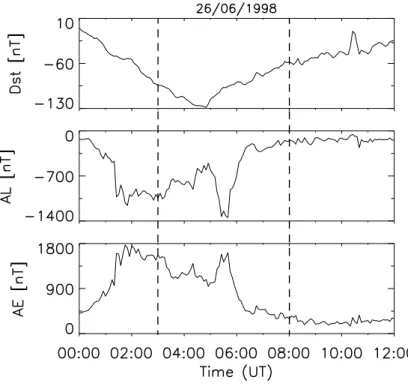
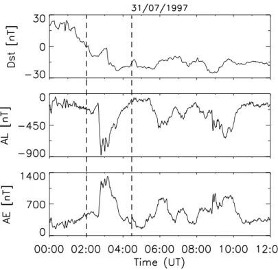
Fig. 1. The AE, AL and Dst-indices

between 00:00 and 12:00 UT on 26 June 1998. AE and AL are calculated from 63 stations between 55 and 76◦ in magnetic latitudes. Dstis calculated

from 24 stations below 40◦in magnetic latitudes. The two vertical dashed lines indicate our time interval with data be-tween 03:00 and 08:00 UT.

we have excluded the PIXIE measurements from regions not covered by UVI.

4 Results 4.1 26 June 1998

The geomagnetic indices AE(63), AL(63) and Dst(24) are

presented in Fig. 1, showing very disturbed conditions dur-ing the early part of this day. Note that the numbers in the parenthesis of 63 and 24, respectively, indicate the number of magnetometer stations included in the calculation of the indices. We have measurements from PIXIE and UVI be-tween 03:00 and 08:00 UT, as indicated by the two verti-cal dashed lines. The main phase of a geomagnetic storm lasted until 04:50 UT, when the Dst(24) index reached a

min-imum of −128 nT and thus, is classified as an intense storm (Gonzalez et al., 1994). At the beginning of the recovery phase, a substorm event took place with the magnitude of the

AE(63) and the AL(63) indices at 05:40 UT exceeding 1600 and −1300 nT, respectively.

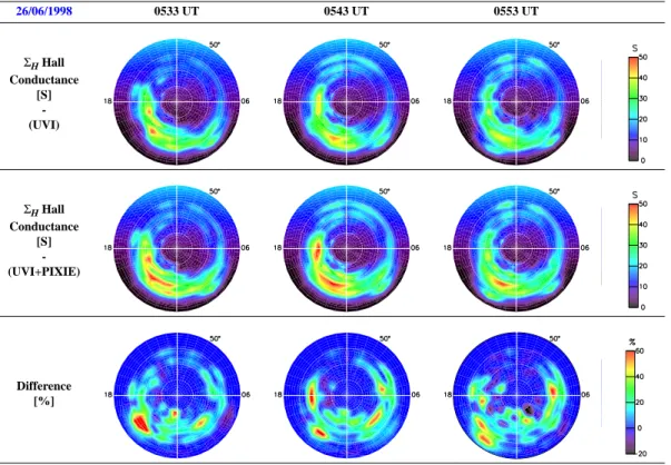
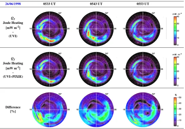
In Fig. 2 we present global maps of the Hall conduc-tance 6H derived during the time period between 05:30 and

06:00 UT on 26 June 1998. The images are 10 min apart, with an integration time of about 4.5 min and the middle time as indicated on top of each column. The upper row con-tains the distribution of the Hall conductance calculated with the AMIE procedure by using magnetometer data and the UVI measurements. In the middle row, the PIXIE data have also been included in the calculation of Hall conductance. We note that the values of Hall conductance are significantly

higher when we make use of the PIXIE data, as the improved spectral characterization of the most energetic electrons has resulted in a larger flux at higher electron energies. This is clearly illustrated by the images in the bottom row, which show the local differences in percent when we take into ac-count the energetic electrons from the PIXIE measurements. We find that the differences in Hall conductance can exceed 60% in some regions when including the PIXIE data. It should be noted, though, that some of the largest differences are found in regions where the Hall conductance values are relatively low. The Pedersen conductance 6P remains more

or less unaffected by the increased electron flux at larger en-ergies, as shown in Fig. 3. By comparing global maps of the Pedersen conductance without the PIXIE data (upper row) with the ones that includes the PIXIE measurements (middle row) for the same time interval, as presented in Fig. 2, we hardly see any difference at all. The images in the bottom row showing the differences in percent tell us that the local variations are generally less than 5%.

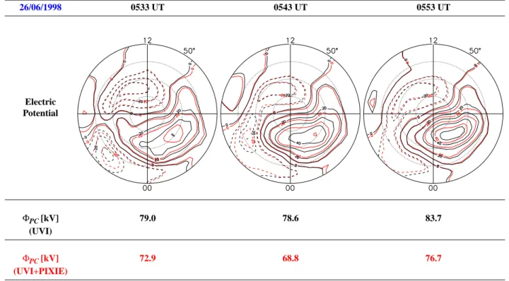
In Fig. 4, we present the distributions of electric potential during the same 3 successive time periods, as in Fig. 2 and Fig. 3. The black lines represent the electric potential pat-tern when we have not included PIXIE data, while the red lines show the situation after taking into account the ener-getic electrons. We note that the general configuration of the patterns remains the same. However, the potential contours shift as the estimated electric field values decrease in regions where the PIXIE data have resulted in a higher Hall conduc-tance. We observe that the lines more or less overlap around noon, consistent with the fact that the images in the bottom row of Fig. 2 show negligible differences in this region when

26/06/1998 0533 UT 0543 UT 0553 UT ΣH Hall Conductance [S] -(UVI) ΣHHall Conductance [S] -(UVI+PIXIE) Difference [%]

Fig. 2. Polar plots of the Hall conductance derived without (upper row) and with (middle row) PIXIE data between 05:30 and 06:00 UT on 26 June 1998. The differences in percent when including the PIXIE data are presented in the bottom row.

26/06/1998 0533 UT 0543 UT 0553 UT ΣP Pedersen Conductance [S] -(UVI) ΣP Pedersen Conductance [S] -(UVI+PIXIE) Difference [%]

Fig. 3. Polar plots of the Pedersen conductance derived without (upper row) and with (middle row) PIXIE data between 05:30 and 06:00 UT on 26 June 1998. The differences in percent when including the PIXIE data are presented in the bottom row.

Electric Potential PC[kV] (UVI) 79.0 78.6 83.7 PC[kV] (UVI+PIXIE) 72.9 68.8 76.7

Fig. 4. Polar plots of the electric potential derived without (black contour lines) and with (red contour lines) PIXIE data between 05:30 and 06:00 UT on 26 June 1998.

including the PIXIE data. However, from the pre-midnight sector until the morning region, we find significant modifica-tions of the electric field strength due to the precipitation of energetic electrons. Below each of the images presented in Fig. 4, we have listed the values of the calculated polar cap potential drop 8P C, showing a clear reduction when

includ-ing the PIXIE measurements.

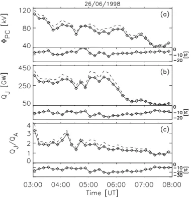
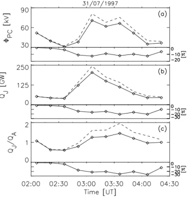
Values of the potential drop during the whole time period when we have measurements from PIXIE and UVI between 03:00 and 08:00 UT on 26 June 1998, are presented in the upper row of Fig. 5a. The dashed line represents the poten-tial drop derived without the PIXIE data, while the solid line gives the values after including the PIXIE measurements. The diamonds give the middle time in each integration pe-riod. We see that the inclusion of energetic electrons causes a reduction in the potential drop. The plot below presents the difference in percent with and without the PIXIE data, show-ing a general decrease between 5 and 10%. In Fig. 5b, we give the values of the Joule heating rate QJ integrated over

the Northern Hemisphere. Similarly to the electric poten-tial, we find that the estimated Joule heating decreases when including the PIXIE measurements. For most of the time pe-riod investigated, the decrease is between 10 and 15%, as shown in the bottom row of Fig. 5b. The larger decrease in Joule heating compared to that in the potential drop is not surprising, as Joule heating QJ depends on the square of the

electric field E according to the formula:

QJ =6PE2. (2)

The inferred energy flux QAby precipitating particles

in-creases when we include the energetic electrons from PIXIE. At most, the increase is about 7% during the time period in-vestigated from the event of 26 June 1998. Since Joule heat-ing decreases when includheat-ing the PIXIE data, we find that the energy flux QA compared with Joule heating QJ becomes

significantly more important. In Fig. 5c, we have plotted the ratio QJ/QA. The dashed line representing the ratios

with-out using the PIXIE data shows the highest ratios. When in-cluding the PIXIE data, the ratio decreases, as shown by the solid line. The difference sometimes exceeds 20%. We note that the ratio is larger than 1 throughout almost the entire pe-riod, meaning that the energy due to Joule heating generally exceeds the energy flux deposited by precipitating particles. However, the difference between Joule heating and energy flux reduces significantly when including the PIXIE data.

From Fig. 5, we can conclude that the maximum change in the hemispheric integrated Joule heating rate from adding PIXIE observations is ∼ 17%. However, there can be much larger decreases in localized regions, as shown in Fig. 6. Here we present global maps of Joule heating, showing lo-cal decreases sometimes exceeding 50% when including the PIXIE data. The changes in Joule heating take place in re-gions where there is a significant flux of energetic electrons. For instance, looking at the images from 05:33 UT, the up-per row shows the strongest Joule heating stretching from about 13:00 until 02:00 MLT. Including the PIXIE data re-sults in significant decreases of approximately 25 and 50% in the pre-midnight sector after 19:00 MLT. This corresponds

Fig. 5. (a) Polar cap potential drop

8P C, (b) Joule heating rate QJand (c)

the ratio QJ/QA between Joule

heat-ing and energy flux estimated through-out the time interval between 03:00 and 08:00 UT on 26 June 1998. The parameters have been calculated with-out (dashed line) and with (solid line) PIXIE data. The differences in per-cent when including PIXIE measure-ments are also presented.

well with the images of the Hall conductance in Fig. 2 from the same time period, showing the largest differences to take place in this pre-midnight sector.

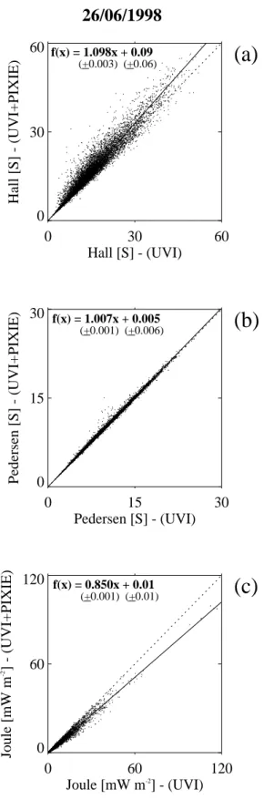
During the whole time period between 03:00 and 08:00 UT on 26 June 1998, when we have PIXIE and UVI measurements, AMIE provides 9058 data values from re-gions covered by both instruments.These values are pre-sented as a scatter plot in Fig. 7, showing the effects of energetic electrons occurring at different levels of tances and Joule heating. The distribution of Hall conduc-tance is given in Fig. 7a in terms of dots, giving the UVI derived values along the horizontal axis and the values when including the PIXIE measurements along the vertical axis. From Fig. 7a, we observe a rather systematic increase in the Hall conductance caused by the inclusion of energetic elec-trons. By performing a simple linear regression analysis, we find that the Hall conductance, on average, increases by 10% when taking into account the PIXIE measurements. This in-crease in the Hall conductance is indicated with the solid line representing a function f (x) having a proportionality factor of 1.098. We also note that in some cases the values dif-fer strongly, exceeding more than 100% when including the PIXIE data in the estimation of the Hall conductance. The dashed line having a proportionality factor of 1.0 is drawn to indicate the locations of the Hall conductance values in cases where the two data sets provide the same output. As inclusion of PIXIE data usually leads to a larger Hall con-ductance, we therefore find 84% of the dots located above the dashed line. In some cases the improved spectral char-acterization at higher energies by using PIXIE data results in a lower electron flux than calculated using extrapolated UVI spectra. This explains the dots located below the dashed line

in Fig. 7a. We should point out that the individual dots rep-resent a significant uncertainty considering the complex pro-cedure to estimate electron energy spectra from combined PIXIE and UVI measurements, as described in Sect. 2. The uncertainties will show up as noise though, and not as a sys-tematic error in our data. Taking the standard deviation on the slope of the regression line of 0.003 into account, we can therefore conclude that a larger estimated Hall conductance is to be expected when including PIXIE data in the calcu-lations. A similar scatter plot is presented in Fig. 7b, giv-ing the Pedersen conductance derived with and without the PIXIE data. Here we observe that almost all the values are located at the dashed line. A proportionality factor of 1.007 means that the Pedersen conductance remains very much un-affected by the increased electron flux at larger energies, in accordance with the results presented in Fig. 3. Effects of energetic electrons occurring at different Joule heating lev-els are presented in Fig. 7c, showing a significant reduction when taking the PIXIE data into account. By performing the linear regression analysis, we find that the Joule heating, on average, decreases by 15%. Though the values vary signifi-cantly, with the largest local decrease exceeding 58%.

In Fig. 8, we present the geomagnetic indices AE(67),

AL(67) and Dst(17) from 31 July 1997. The measurements

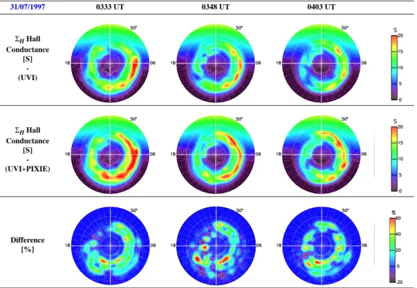
from PIXIE and UVI covering the time period between 02:00 and 04:20 UT involve a clear and isolated substorm event. An abrupt intensification was seen in the AE and AL in-dices around 02:45 UT, with peak values exceeding 1300 and −800 nT, respectively. In Fig. 9 we present three suc-cessive images of the distribution of Hall conductance from the later phases of the substorm, when the conductance max-imum takes place on the morning side. We find that the high

QJ Joule Heating [mW m-2] -(UVI) Q_J Joule Heating [mW m-2] -(UVI+PIXIE) Difference [%]

Fig. 6. Polar plots of Joule heating derived without (upper row) and with (middle row) PIXIE data between 05:30 and 06:00 UT on 26 June, 1998. The differences in percent when including the PIXIE data are presented in the bottom row.

energy electrons derived from the PIXIE data strongly in-crease the Hall conductance, in accordance with the results from the event on 26 June 1998.

Similarly, we find that the estimated Joule heating de-creases, as presented in Fig. 10. In the upper row, where the PIXIE data have not been included, the images show max-ima in both the postnoon sector as well as the morning sec-tor. After including the energetic electrons from PIXIE, the images in the middle row reveal that the Joule heating maxi-mum in the morning sector decreases significantly. However, the maximum in the afternoon sector remains fairly unaf-fected, as the precipitation of energetic electrons is negligible in these regions, according to Fig. 9.

Figure 11 shows the same trends as Fig. 5. Both the calcu-lated potential drop and Joule heating are reduced when we take into account the energetic electrons. During the most active period after 02:45 UT, the potential drop decreases by as much as 13%, while the Joule heating at two occasions de-creases more than 20%. The inferred energy flux inde-creases in general around 5% when including the PIXIE data, resulting in a decrease in the ratio between Joule heating and energy flux by 20 to 30%.

4.2 31 July 1997

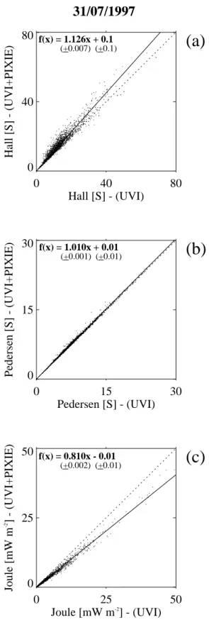
A scatter plot of the Hall conductance values given in Fig. 12a shows the distribution of the 1964 data values AMIE provides between 02:00 and 04:20 UT on 31 July 1997.

The linear regression analysis reveals that the Hall conduc-tance, on average, increases by 13% and with a maximum local increase of 99% when including the PIXIE measure-ments. The Pedersen conductance in Fig. 12b remains more or less unaffected by the energetic electrons, in accordance with the results presented in Fig. 3 and Fig. 7b. A reduc-tion by 19% and a maximum local decrease of about 39% is found in Fig. 12c when studying the PIXIE effects on the Joule heating values.

4.3 28 August 1997

The geomagnetic indices AE(68), AL(68) and Dst(16) from

28 August 1997 are presented in Fig. 13. During the time interval between 03:00 and 10:00 UT when measure-ments from PIXIE and UVI were available, two relatively clear peaks can be seen in the AE(68) and AL(68) in-dices. The first intensification is rather extended in time from about 03:30 until 06:00 UT, with AE exceeding 900 nT and AL reaching −700 nT. This substorm took place dur-ing the main phase of a minor geomagnetic storm, as the

Dst(16) decreased from around −5 nT at 03:00 UT to around −48 nT at 05:30 UT. Then the recovery phase commenced, as the Dst(16) index started to increase. However, around

07:00 UT, another intensification was observed as the mag-nitude of the AE(68) and AL(68) indices increased sig-nificantly, reaching almost 1100 and −800 nT, respectively, around 07:55 UT. Thereafter, the activity slowly diminished.

26/06/1998

0

60

120

Joule [mW m

] - (UVI)

0

60

120

Joule [mW m

] - (UVI+PIXIE)

(c)

0

15

30

Pedersen [S] - (UVI)

0

15

30

Pedersen [S] - (UVI+PIXIE)

(b)

0

30

60

Hall [S] - (UVI)

0

30

60

Hall [S] - (UVI+PIXIE)

(a)

Fig. 7. (a) Hall conductances 6_H, (b) Pedersen conductances 6_P and (c) Joule heating values QJderived with and without the PIXIE

data throughout the time interval between 03:00 and 08:00 UT on 26 June 1998. The data values are taken from the regions covered by the PIXIE and UVI instruments. The solid line results from a linear regression analysis of the data points.

In Fig. 14 we present similar plots, as presented in Fig. 5 and Fig. 11. Again we note the effects of the energetic elec-trons on polar cap potential, Joule heating and energy flux. Overall, the effects are less than the ones found during the event on 26 June 1998, and 31 July 1997. According to Fig. 14a, the calculated potential drop is generally reduced by 5% at most for the first geomagnetic disturbed period be-tween 03:00 and 06:00 UT. The inferred Joule heating de-creases by 5 to 10% during the same period, as shown in Fig. 14b. However, the second intensification after 07:00 UT seen in Fig. 13 results in relatively large effects. Figure 14c reveals that the ratio between Joule heating and energy flux is reduced by about 25% around 08:30 UT. Similar to Fig. 7 and Fig. 12, we also present in Fig. 15 the distribution of conductances and Joule heating values for the 5767 data val-ues provided by AMIE between 03:00 and 10:00 UT on 28 August 1997.

By performing the linear regression analysis, we derive an average increase of the Hall conductance of 7.4%, as given in Fig. 15a. This result is somewhat lower than the correspond-ing values of 10 and 13% from the events of 26 June 1998, and 31 July 1997, respectively. Figure 15 further shows that the decrease in the Joule heating values caused by the en-ergetic electrons, on average, reaches 15%, while the Peder-sen conductance remains practically unaffected by the PIXIE data.

5 Discussion

We have studied the effects of energetic electrons on iono-spheric electrodynamics during periods of substorm activity occurring on 31 July and 28 August 1997, and 26 June 1998. On 31 July 1997, we have measurements prior to and during an isolated substorm event. Before substorm onset around 02:40 UT, the PIXIE effects are minor, as shown in Fig. 11. This indicates that the growth phase was dominated by less energetic particles, in accordance with the statistical study by Østgaard et al. (1999) presented in Sect. 1. Fig-ure 11 further shows that the effects of energetic electrons increase as the expansion phase commences. Østgaard et al. (2001) and Aksnes et al. (2002) have investigated this sub-storm event thoroughly, showing an eastward drift of the en-ergetic electrons and the development of a maximum in the morning sector during the recovery phase of the substorm. This explains the significant effects of energetic electrons re-ducing the estimated Joule heating integrated over the North-ern Hemisphere by more than 20% and the ratio between Joule heating and energy flux by almost 30%. On 26 June 1998, the effects of energetic electrons are largest during the substorm event between 05:00 and 06:00 UT, according to Fig. 5. From Fig. 2, we now observe a shift westward of the Hall conductance maximum. At 05:33 UT, the maximum is located around 19:00 MLT. Ten minutes later, we find the largest Hall conductance in the MLT sector 17–18. This shift westward may be associated with a westward travelling surge (WTS). Ground magnetometer data from the station Barrow

Fig. 8. The AE, AL and Dst-indices

between 00:00 and 12:00 UT on 31 July 1997. AE and AL are calculated from 67 stations between 55 and 76◦in mag-netic latitudes. Dst is calculated from

17 stations below 40◦in magnetic lat-itudes. The two vertical dashed lines indicate our time interval with data be-tween 02:00 and 04:20 UT.

indicate the appearance of a WTS, as we observe typical fea-tures like a negative dip in the H component and a positive bay in the Y component. As summarized by Miller and Von-drak (1985), WTS is associated with energetic electrons.

In Fig. 14, we show effects of energetic electrons on iono-spheric electrodynamics during the event of 28 August 1997. The second intensification starting around 07:00 UT results in large differences, in accordance with the results from 31 July 1997, and 26 June 1998. However, we also note that the first intensification this day between 03:00 and 06:00 UT only leads to minor differences. Except for the results around 04:30 UT, the effects of energetic electrons are less than we might have expected when observing the relatively large in-crease in the geomagnetic indices. This results from the fact that the precipitating electrons were mostly less ener-getic during this time period. We note that the AE and AL indices peaked at about 900 nT and −700 nT, respectively. During the second intensification on 28 August, the AE in-dex reached almost 1100 nT and the AL inin-dex was close to

−800 nT. The two other events from 31 July and 26 June both show much larger values of the AE and AL indices, as presented in Fig. 1 and Fig. 8.

In Fig. 16a we give an example of a typical precipitat-ing electron energy spectrum derived from PIXIE and UVI measurements.The solid line represents the full spectral char-acterization where both PIXIE and UVI data are taken into account. While the lower electron energies are determined from UVI data, the PIXIE measurements enable us to char-acterize the most energetic electrons. Also plotted is a dashed line showing the situation without PIXIE data, where the UVI derived electron spectrum has been extrapolated to-wards higher energies. Such an extrapolation is obviously

not sufficient here, as we see a significant drop in the elec-tron flux at higher energies. As pointed out in Sect. 1, the PIXIE data may sometimes reveal a lower electron flux at higher energies than provided by the extrapolated UVI spec-tra. This explains the cases with negative differences when including PIXIE data in Figs. 2, 3, 7, 9, 12, and 15. Never-theless, from the same figures we can conclude that the sit-uation presented in Fig. 16a, showing a higher electron flux when including PIXIE data, is by far the most typical. In Fig. 16b we present the effects on the electron energy depo-sition from the two situations described in Fig. 16a with and without PIXIE data. The dashed line giving the height profile of the electron energy deposition based on the extrapolated UVI derived spectrum falls off steeply below 100 km. At al-titudes lower than 90 km, the electron energy deposition val-ues are practically insignificant, as the valval-ues have dropped below 10 keV·cm−3_·s−1_{. In comparison, the solid line}

rep-resenting the energy deposition from the electron spectrum derived using combined PIXIE and UVI measurements re-mains large in the upper part of the D-region and first starts to fall off drastically below 80 km. We find that including PIXIE data increases the total height-integrated energy de-position by about 40%. However, if we only consider the region below 100 km, the increase is more than 600%.

In Fig. 16c, we present similar height profiles of the Hall conductance. We note the discrepancy below 100 km, result-ing in a large difference in the total height-integrated Hall conductivity. Without PIXIE data, we derive a Hall con-ductance of 27 S. By including the information from the X-ray measurements, the resulting Hall conductance value is 39 S, an increase of ∼44%. The importance of the energetic electrons for the Hall conductance has been pointed out by

31/07/1997 0333 UT 0348 UT 0403 UT ΣH Hall Conductance [S] -(UVI) ΣH Hall Conductance [S] -(UVI+PIXIE) Difference [%]

Fig. 9. Polar plots of the Hall conductance derived without (upper row) and with (middle row) PIXIE data between 03:30 and 04:05 UT on 31 July 1997. The differences in percent when including the PIXIE data are presented in the bottom row.

31/07/1997 0333 UT 0348 UT 0403 UT QJ Joule Heating [mW m-2] -(UVI) QJ Joule Heating [mW m-2] -(UVI+PIXIE) Difference [%]

Fig. 10. Polar plots of Joule heating derived without (upper row) and with (middle row) PIXIE data between 03:30 and 04:05 UT on 31 July 1997. The differences in percent when including the PIXIE data are presented in the bottom row.

Fig. 11. (a) Polar cap potential drop

8P C, (b) Joule heating rate QJand (c)

the ratio QJ/QA between Joule

heat-ing and energy flux estimated through-out the time interval between 02:00 and 04:20 UT on 31 July 1997. The parameters have been calculated with-out (dashed line) and with (solid line) PIXIE data. The differences in per-cent when including PIXIE measure-ments are also presented.

Schlegel (1988). From two years of EISCAT data, 8337 con-ductivity profiles were calculated within a height region be-tween 90 and 180 km. The maximum Hall conductivity was usually located at 109 km. In comparison, the largest Hall conductivity in Fig. 16c is at an altitude of 108 km, along with a significant contribution to the Hall conductance at lower heights. During times with very energetic particle pre-cipitation, Schlegel sometimes found the maximum in Hall conductance at heights below 100 km. For such events, the conductivity profiles were extrapolated exponentially down to 75 km altitude, in order to derive a more accurate height-integrated Hall conductivity.

From Fig. 16, we can conclude that the difference between including PIXIE data or not may be tremendous in the lower E-region below 100 km. Significant effects on physical pro-cesses in the lower thermosphere and mesosphere should be expected. When interpreting the results found in this study, though, we need to keep in mind the limitations described in Sect. 2.5. First of all, the rather coarse PIXIE resolution (600–900 km) prevents us from identifying localized struc-tures in the electron precipitation. Secondly, the procedure for establishing electron spectra and thereafter calculating ionospheric conductances from PIXIE and UVI measure-ments may also be a source of uncertainty. As explained in Sect. 2.4., several assumptions and relations have been in-corporated in the computer code used to infer height profiles of the ionization. We should therefore be careful when dis-cussing ionospheric effects at specific altitudes from the in-vestigation performed. Nevertheless, the results presented in Sect. 4. undoubtedly indicate that the inclusion of PIXIE data may have a large effect on the ionospheric electrodynamics.

5.1 Effects on the electric field

The large-scale ionospheric electric field has its origin in the interaction between the magnetosphere and the solar wind, and its configuration depends on the conditions of the inter-planetary magnetic field (IMF). During periods of a south-ward pointing IMF, a two-cell electric convection pattern is established at higher latitudes. The electric potential drop across the polar cap is calculated as the difference between the minimum and maximum electric potentials and is often used to compare different electrodynamical states. Particle precipitation leads to an enhancement of ionospheric conduc-tivities, resulting in electric polarization fields and thereby a modification of the electric field in the ionosphere locally (Bostrøm, 1973). Significant increases in the Hall conduc-tance when including the PIXIE data during periods of sub-storm activity are seen in Figs. 2 and 9. The largest local effects of energetic electrons on the Hall conductances reach about 100%, as shown in Fig. 7a, Figs. 12a and 15a. By as-suming that the magnetosphere acts as a current generator, the computational effect of a larger Hall conductance from the AMIE calculations is a reduction of the estimated elec-tric field. This has been shown in Figs. 4a, 11a and 14a. Such an anticorrelation between Hall conductance and iono-spheric electric field has been reported in several papers us-ing measurements from rockets (Wescott et al., 1969; Went-worth, 1970; Evans et al., 1977; Marklund et al., 1982), satel-lites (Shue and Weimer, 1994; Johnson et al., 1998), and radars (de la Beaujardi`ere et al., 1977; Kirkwood et al., 1988; Opgenoorth et al., 1990; Aikio et al., 1993; Lanchester et al., 1996).

31/07/1997

0

25

50

Joule [mW m

_{] - (UVI)}

0

25

50

Joule [mW m

] - (UVI+PIXIE)

(c)

0

15

30

Pedersen [S] - (UVI)

0

15

30

Pedersen [S] - (UVI+PIXIE)

(b)

0

40

80

Hall [S] - (UVI)

0

40

80

Hall [S] - (UVI+PIXIE)

(a)

Fig. 12. (a) Hall conductances 6_H, (b) Pedersen conductances 6_P and (c) Joule heating values QJderived with and without the PIXIE

data throughout the time interval between 02:00 and 04:20 UT on 31 July 1997. The data values are taken from the regions covered by the PIXIE and UVI instruments. The solid line results from a linear regression analysis of the data points.

5.2 Effects of proton precipitation

The UVI camera is potentially sensitive to protons, as men-tioned in Sect. 2.2. According to Frey et al. (2001), LBH emissions may contain contributions from proton excitation, though, this should be limited to regions with strong pro-ton precipitation. Particle observations from polar orbiting satellites (Hardy et al., 1989, 1991; Newell et al., 1991) and ground-based optical H emission observations (Creutzberg et al., 1988) show that the proton aurora can be of particular importance in the cusp and at the equatorward boundary of the auroral oval before midnight. Even though the statistical studies by Hardy et al. (1989) and Galand et al. (2001) show that electrons are the dominant source of ionization, protons, on average, contribute ∼ 15% to the total energy inferred. Protons precipitating in the atmosphere are treated as elec-trons in the UVI calculations, as the measured UV-emissions are assumed to be caused by precipitating electrons. This may lead to an underestimation of the electron density, ac-cording to a study by Galand et al. (1999). Galand et al. (1999) investigated the ionization by energetic protons in the auroral atmosphere using the Thermosphere-Ionosphere Electrodynamics General Circulation Model (Richmond et al., 1992). First, they calculated the ionospheric ionization caused by proton precipitation. Then they treated the protons as electrons, and showed that the resulting electron density was being underestimated. The largest difference occurred around 130 km, near the region where the Pedersen conduc-tivity peaks. This indicates that the Pedersen conductance may change somewhat when treating protons as electrons. A proton with an energy of 10 keV will deposit most of its en-ergy in this height region around 130 km (Rees, 1982). In comparison, an electron with a similar energy of 10 keV can penetrate down below 110 km (Rees, 1963). For a proton to penetrate down to approximately 105 km where the Hall con-ductivity is largest, an energy of almost 100 keV is needed (Rees, 1982). According to Hardy et al. (1989) the proton aurora can typically be expressed as a Maxwellian with a characteristic energy between 1 and 20 keV, indicating that the Hall conductance, in general, should be more or less un-affected by proton precipitation. If we assume that precipi-tating protons takes place during the three events of 31 July and 28 August 1997, and 26 June 1998, this might affect the calculation of Pedersen conductance. However, the possible change in the Pedersen conductance should be the same for a calculation with and without the PIXIE data, meaning that the proton aurora should not affect the results presented in this study. In order for proton precipitation to make a signif-icant impact on the results, we need precipitating protons in the energy range of 100 keV or more. Since the protons do not produce measurable X-rays because of their large mass compared with electrons, we might underestimate the Hall conductance during such a situation. Taking energetic pro-tons in the energy range of 100 keV into account, we should then find the effects presented in Sect. 4 to be slightly larger.

Fig. 13. The AE, AL and Dst-indices

between 00:00 and 12:00 UT on 28 Au-gust 1997. AE and AL are calculated from 68 stations between 55 and 76◦ in magnetic latitudes. Dstis calculated

from 16 stations below 40◦in magnetic latitudes. The two vertical dashed lines indicate our time interval with data be-tween 03:00 and 10:00 UT.

Fig. 14. (a) Polar cap potential drop

8P C, (b) Joule heating rate QJand (c)

the ratio QJ/QA between Joule

heat-ing and energy flux estimated through-out the time interval between 03:00 and 10:00 UT on 28 August 1997. The parameters have been calculated with-out (dashed line) and with (solid line) PIXIE data. The differences in per-cent when including PIXIE measure-ments are also presented.

28/08/1997

0

15

30

Joule [mW m

] - (UVI)

0

15

30

Joule [mW m

] - (UVI+PIXIE)

(c)

0

10

20

Pedersen [S] - (UVI)

0

10

20

Pedersen [S] - (UVI+PIXIE)

(b)

0

20

40

Hall [S] - (UVI)

0

20

40

Hall [S] - (UVI+PIXIE)

(a)

Fig. 15. (a) Hall conductances 6H, (b) Pedersen conductances 6P

and (c) Joule heating values QJderived with and without the PIXIE

data throughout the time interval between 03:00 and 10:00 UT on 28 August, 1997. The data values are taken from the regions covered by the PIXIE and UVI instruments. The solid line results from a linear regression analysis of the data points.

5.3 Joule Heating vs. AE

Several studies have investigated and found a nearly linear re-lationship between hemispheric integrated Joule heating and the AE index. Such studies are motivated by the fact that we are often only able to provide Joule heating in localized regions. A possible relation with a geomagnetic index like

AEmeans we can estimate Joule heating continuously over the entire polar region. Papers report a proportionality fac-tor between the Joule heating rate and the AE index rang-ing from 0.16 to 0.54 GW/nT (Ahn et al., 1983b; Baumjo-hann and Kamide, 1984; Richmond et al., 1990; Cooper et al., 1995; Lu et al., 1996, 1998). The discrepancy be-tween the studies may be attributed to the fact that different methods are used to obtain Joule heating and the AE index. Both Ahn et al. (1983b) and Baumjohann and Kamide (1984) used the Kamide-Richmond-Matsushita algorithm (Kamide et al., 1981). However, while Ahn et al. (1983b) derived the conductances on the basis of ground magnetic perturbations, Baumjohann and Kamide made use of an improved version (Kamide et al., 1982) of the statistical conductance model developed by Spiro et al. (1982). Like the study presented in this paper, Richmond et al. (1990), Cooper et al. (1995) and Lu et al. (1996, 1998) applied the AMIE procedure. Though Richmond et al. adopted AE(12) in their analysis, the other papers calculated AE from the north-south component of the magnetic perturbations measured by all available mag-netometer stations in the high-latitude auroral zone. Cooper et al. estimated a proportionality factor of 0.54 GW/nT when using AE(12). However, when using a multistation-derived

AEfrom AMIE, they found the relation between Joule heat-ing and the AE index to be 0.28 GW/nT.

We have done a similar investigation with the studies de-scribed here, by performing a linear regression analysis. When using the Joule heating derived without the PIXIE data, we find the proportionality factors to vary between 0.15 and 0.26, meaning that we are in the lower end of the results found by others. Including the effects of energetic electrons results in even lower proportionality factors, as presented in Fig. 17.

For the events of 31 July and 28 August 1997, we find proportionality factors of 0.15 and 0.13 GW/nT, respectively. On 26 June 1998, we obtain a somewhat larger value of 0.23 GW/nT. While the isolated substorm event of 31 July takes place during a non-storm period and the event of 28 August occurs during a minor geomagnetic storm, the sub-storm activity investigated on 26 June is related to a se-vere storm with the Dst index reaching a minimum value

of −128 nT. The large proportionality factor established be-tween the Joule heating and the AE index for the event of 26 June may be attributed to the intense geomagnetic storm condition for this date. A characteristic of a geomagnetic storm is a strong convective electric field (Gonzalez et al., 1994), indicating that the electric field may contribute more to the ionospheric current responsible for the AE values dur-ing storms than durdur-ing non-storm conditions. As Joule heat-ing depends strongly on the electric field strength, we should

UVI

UVI

-PIXIE

extrapolated

Fig. 16. (a) An example of a typi-cal precipitating electron energy spec-trum derived using UVI data at lower electron energies (solid line) and then PIXIE data at higher energies (solid line) and an extrapolation of the UVI derived electron spectrum (dashed line). (b) Height profiles showing the electron energy deposition for the two situations presented in (a). (c) Height profiles of the Hall conductivity for the two situa-tions presented in (a).

therefore expect a larger ratio between Joule heating and AE index during storm periods. When looking at the different papers investigating this relationship using the AMIE proce-dure, we find such a tendency. Richmond et al. (1990) and Lu et al. (1996) study non-storm events and find proportion-ality factors ranging between 0.16 and 0.21 GW/nT. Cooper et al. (1995) and Lu et al. (1998) find larger values between 0.25 and 0.54 GW/nT when studying storm events. A more thorough investigation is needed, though, for this suggested relationship between Joule heating, AE index and geomag-netic storm condition.

From Fig. 17, we see that the linear correlation coefficient

ris high for all events, ranging from 0.88 to 0.94. However, we should point out that the number of points is limited. For the events on 28 August 1997, and 26 June 1998, we have 34 and 30 data points, respectively. From the isolated substorm event on 31 July 1997, we have only 10 values. Therefore, one must be cautious when interpreting the results. Even though the statistics are rather limited, the results neverthe-less show that the Joule heating turns out to be lower than previous studies have reported. The events of 31 July and 28 August, operating with proportionality factors of 0.15 and 0.13 GW/nT, respectively, provide lower values for the rela-tionship between Joule heating and AE than found by oth-ers studying non-storm events. Likewise, the proportionality factor of 0.23 GW/nT for the event of 26 June is less than

that found by previous studies using data from storm time conditions.

5.4 Effects on energy budget

We have found that the inferred Joule heating integrated over the Northern Hemisphere decreases by up to 20 percent when energetic electrons are taken into account. According to Fig. 5c, Fig. 11c and Fig. 14c, the ratio between Joule heating and electron energy flux decreases even more, as the calcu-lated energy flux increases when we include the PIXIE data. These results show that auroral energy input by precipitating particles probably contributes relatively more to the total en-ergy budget than previous papers have reported. One of the fundamental questions in space physics involves the energy coupling between the solar wind and the Earth’s magneto-sphere. The energy budget during magnetic storms and sub-storms has been evaluated and presented in several papers in the literature (Akasofu, 1981; Harel et al., 1981; Stern, 1984; Tsurutani and Gonzalez, 1995; Lu et al., 1995, 1998; Knipp et al., 1998; Østgaard et al., 2002a). The studies agree that the most important forms of energy dissipation in the near-Earth space are the magnetospheric ring current injec-tion, atmospheric Joule heating and the energy flux carried by precipitating particles. However, the relative importance of the different energy forms is still much argued. Most studies

0

300

600

900

1200

1500

AE index [nT]

0

50

100

150

200

250

300

Joule Heating [GW]

0

375

750

1125

1500

AE index [nT]

0

50

100

150

200

Joule Heating [GW]

0

400

800

1200

1600

2000

AE index [nT]

0

100

200

300

400

Joule Heating [GW]

Fig. 17. The relationship between Joule heating and the AE index for the peri-ods with substorm activity occurring on (a) 31 July 1997 (b) 28 August 1997, and (c) 26 June 1998. Note that the PIXIE data have been included when deriving Joule heating presented here. The solid line in each plot represents the result from the linear regression an-alyze.

report that Joule heating represents by far the largest iono-spheric energy sink to the total energy budget. Atmoiono-spheric heating can affect thermospheric winds and cause vertical motions which, in turn, change the atmospheric composition. Another possible effect is the expansion of the atmosphere resulting in increasing atmospheric drag on near-Earth satel-lites (AFSPCPAM15-2, 1997). Even though we usually find Joule heating to be higher than the precipitating electron en-ergy flux, our result strongly indicates that the contribution from auroral particles is more important than that presented in most studies considering the energy budget. This is in accordance with a recent paper by Østgaard et al. (2002b).

They have investigated the energy dissipation rate during 7 substorms from 1997 by using observations from PIXIE and UVI. Nonlinear relations between the energy flux and the AE and AL indices have been established and compared with similar linear relations performed by others. The result by Østgaard et al. (2002b) is much in accordance with a paper by Lu et al. (1998). However, Østgaard et al. (2002b) find values which are a factor 1–2 times larger than the results by Spiro et al. (1982) and Richmond (1990), and about 4 times larger than reported in studies by Akasofu (1981) and Ahn et al. (1983b).

Hall conductance and Joule heating are found in regions of limited extent, as demonstrated in Fig. 2, Fig. 6, Fig. 9, and Fig. 10. We have excluded values less than 10 S and 10 mWm−2, respectively, to avoid effects caused by statistical uncertainties.

Largest effects of energetic electrons during the event of: 31 July 1997 28 August 1997 26 June 1998 02:00–04:20 UT 03:00–10:00 UT 03:00–08:00 UT Local Hall Conductance 16H 99% 84% 138%

Local Joule Heating 1QJ -39% -47% -58%

Polar Cap Potential Drop 18_{P C} -13% -9.2% -12% Hemispheric Integrated Joule Heating 1QJ -21% -20% -17%

Hemispheric Integrated Energy Flux 1Q_A 8.6% 6.7% 7.4% Radio Between Joule Heating and Energy Flux 1QJ/QA) -27% -25% -22%

In Figs. 5c, 11c and 14c, the ratio between the hemispheric integrated Joule heating QJ and energy flux by precipitating

particles QA is presented. By integrating the total

contribu-tions from these two ionospheric energy forms throughout the respective time periods with measurements and then cal-culating the ratio QJ/QA, we estimate the largest ratio of

1.67 for the severe storm event of 26 June 1998. This value is much larger than the corresponding average ratios of 1.04 and 0.955 for the events of 31 July and 28 August 1997, in-dicating that the energy flux by the precipitating particles is of special importance for substorm events occurring during non-storm periods or minor geomagnetic storms. It is in-teresting to note that an inclusion of the neutral wind in the AMIE calculations would probably lead to less Joule heating values and, therefore, even lower ratios between Joule heat-ing and energy flux by precipitatheat-ing particles. Lu et al. (1995) investigated the effects of neutral wind on Joule heating for 28–29 March 1992, when several intensifications could be seen in the AE index. On the average, for this two-day pe-riod, the hemispheric integrated Joule heating was reduced by 28 percent due to the neutral wind.

6 Conclusion

In this study we have investigated the effects of energetic electrons on ionospheric electrodynamics. This was done by running the AMIE procedure using UVI and magnetometer data and then investigating energetic electrons by repeating the study and including PIXIE data. We find that the im-proved spectral characterization of the precipitating electrons using PIXIE data most often results in a larger electron flux at higher energies and consequently, a higher Hall conduc-tance. The increased Hall conductance then leads to a re-duction in the estimated electric field, and we find that the calculated polar cap potential drop sometimes decreases by more than 10% during geomagnetic disturbed periods. This further affects the estimation of Joule heating, which may be 20% lower on a global scale. In some localized regions, Joule heating can decrease by more than 50%. Including the

PIXIE data increases the energy flux of precipitating particles by approximately 5%, resulting in a decrease in the calcu-lated ratio between Joule heating and energy flux, sometimes by more than 25%. The largest estimated effects of ener-getic electrons during the three events studied in this paper are presented in Table 1.

We note that the inclusion of the PIXIE data affects the calculation of Hall conductance, polar cap potential, Joule heating and energy flux, while the estimated Pedersen con-ductance is hardly affected at all.

The relationship between Joule heating and the AE index has also been studied in this paper. In accordance with pre-vious studies, we find a nearly linear relationship between these two quantities. However, our investigation gives pro-portionality factors between Joule heating and the AE in-dex ranging from 0.13 and 0.23 GW/nT. We suggest that the largest value of 0.23 GW/nT derived from the event of 26 June 1998, may be attributed to the geomagnetic storm conditions during this day. A more thorough investigation is needed, though, for this proposed relationship, as only three events have been studied in this paper. By comparing our data with the results found by others considering storm and non-storm conditions, respectively, we obtain lower values of the ratio between Joule heating and AE index than reported in previous studies. An investigation has also been performed regarding the relative importance of the ionospheric energy sinks. For the severe storm event of 26 June 1998, the hemi-spheric integrated Joule heating represents the largest energy form and contributes 1.67 times more than the hemispheric integrated energy flux by precipitating particles. However, corresponding ratios of 1.04 and 0.955 are found for the events of 31 July and 28 August 1997, indicating the impor-tance of the auroral particle precipitation to the energy bud-get for substorm events occurring during non-storm or minor geomagnetic storm periods.

Acknowledgements. This study was supported by the Research

Council of Norway (NFR).

A. Aksnes thanks HAO/NCAR for their hospitality and support dur-ing a three-months stay in 2002.