Towards improving the electroanalytical speciation analysis of indium

HAL Id: hal-01950315

https://hal.archives-ouvertes.fr/hal-01950315

HAL is a multi-disciplinary open access archive for the deposit and dissemination of sci-entific research documents, whether they are pub-lished or not. The documents may come from teaching and research institutions in France or abroad, or from public or private research centers.

L’archive ouverte pluridisciplinaire HAL, est destinée au dépôt et à la diffusion de documents scientifiques de niveau recherche, publiés ou non, émanant des établissements d’enseignement et de recherche français ou étrangers, des laboratoires publics ou privés.

analysis of indium

Élise Rotureau, Pepita Pla-Vilanova, Josep Galceran, Encarna Companys,

Jose Paulo Pinheiro

To cite this version:

Élise Rotureau, Pepita Pla-Vilanova, Josep Galceran, Encarna Companys, Jose Paulo Pinheiro. To-wards improving the electroanalytical speciation analysis of indium. Analytica Chimica Acta, Elsevier Masson, 2019, 1052, pp.57-64. �10.1016/j.aca.2018.11.061�. �hal-01950315�

1

Towards improving the electroanalytical

2

speciation analysis of indium

3

4

Elise Rotureau*

_{, Pepita Pla-Vilanova}

_{, Josep Galceran}

_{, Encarna Companys}

_,

5

José Paulo Pinheiro

6

7

1 _{CNRS, LIEC (Laboratoire Interdisciplinaire des Environnements Continentaux), UMR7360,}

8

Vandoeuvre-lès-Nancy F54501, France. 9

2 _{Université de Lorraine, LIEC, UMR7360, Vandoeuvre-lès-Nancy F54501, France.}

10

3 _{Departament de Química, Universitat de Lleida and AGROTECNIO, Rovira Roure 191,}

11

25198 Lleida, Catalonia, Spain 12

13

Keywords: indium, free metal, AGNES, SCP, electroanalytical techniques, speciation

14 15 16 17 18

ABSTRACT

19

The geochemical fate of indium in natural waters is still poorly understood, while recent 20

studies have pointed out a growing input of this trivalent element in the environment as a 21

result of its utilisation in the manufacturing of high-technology products. Reliable and easy-22

handling analytical tools for indium speciation analysis is, then, required. In this work, we 23

report the possibility of measuring the total and free indium concentrations in solution using 24

two complementary electroanalytical techniques, SCP (Stripping chronopotentiometry) and 25

AGNES (Absence of Gradients and Nernstian Equilibrium Stripping) implemented with the 26

TMF/RDE (Thin Mercury Film/Rotating Disk Electrode). Nanomolar limits of detection, i.e. 27

0.5 nM for SCP and 0.1 nM for AGNES, were obtained for both techniques in the 28

experimental conditions used in this work and can be further improved enduring longer 29

experiment times. We also verified that AGNES was able (i) to provide robust speciation data 30

with the known In-oxalate systems and (ii) to elaborate indium binding isotherms in presence 31

of humic acids extending over 4 decades of free indium concentrations. 32

The development of electroanalytical techniques for indium speciation opens up new routes 33

for using indium as a potential tracer for biogeochemical processes of trivalent elements in 34

aquifers, e.g. metal binding to colloidal phases, adsorption onto (bio)surfaces, etc. 35

1. Introduction

36

In the context of extensive expansion of low-carbon energy technologies, indium has been 37

classified by the EU commission as a near-critical metal regarding the risk of supply chain 38

bottlenecks [1]. The principal industrial application of indium worldwide is for producing 39

indium oxide (In2O3) and indium tin oxide (ITO) to make electrically conducting transparent

40

thin films, mainly used for liquid crystal displays and photovoltaic cells. The world’s indium 41

production has increased tenfold since the nineties [2]. Indium is almost exclusively obtained 42

as a by-product in zinc smelters operating using sphalerite (a zinc sulphide ore mineral). 43

Besides, the potential of indium recyclability is relatively limited [3]. It is now recognized that 44

the steadily increased use of indium for technology applications is leading to a significant 45

anthropogenic input in the biogeochemical cycle of indium [4]. While measured total amounts 46

of indium in freshwaters are usually low e.g. ranging from 1 to 15 pM in Japanese rivers [5], 47

more abundant concentrations are found in (i) groundwaters, with reported values of 81 nM 48

and 0.18 µM in Canada [6] and in a polluted site in Taiwan [7], respectively, (ii) acid mine 49

drainage waters, where the amount may reach up to 0.25 µM [8] (iii), soils with measured 50

average values of 0.15 µmol kg-1 [9] and (iv) sediments, with measured values ranging from 51

0.13 to 0.87 µmol kg-1 [10]. 52

In recent years, there is a growing interest in the environmental fate [6,9] and toxicity [11–13] 53

of indium, but they remain mostly unknown [4]. The aqueous geochemistry of indium is very 54

close to other trivalent ions such as gallium and scandium, elements that are all heavily 55

influenced by hydrolysis reactions [14]. In aqueous solution, indium acts as a hard acid which 56

preferentially interacts with ligands containing oxygen donor atoms, e.g. hydroxides, 57

carboxylate and phenolate groups. As for other metal cations, the fate of indium will likely be 58

controlled by its interaction with natural organic matter (NOM) and/or with the mineral 59

surfaces, mostly clays or iron hydro-oxides [15]. Since the understanding of metal speciation is 60

considered as a key issue for evaluating the adverse effects of metallic contamination in natural 61

ecosystems and especially in aquifers, and there are growing demands for on-site indium 62

detection, robust and versatile techniques for laboratory set-up need to be urgently developed. 63

To date, analytical determinations of indium in the environment are commonly performed using 64

inductively coupled spectroscopy and atomic absorption spectroscopy preceded usually by a 65

pre-concentration step [4]. Therefore, current efforts are made to conceive new techniques 66

trying to minimize handling steps before the measurement of free or total indium concentrations 67

in aqueous samples. Among them, ion selective electrodes have been successfully designed 68

with organic solid-contact indium sensors reaching the detection threshold of 0.1 µM [16,17]. 69

Electroanalytical sensors offer great opportunities to quantify the total indium amount at 70

micromolar concentrations levels, using ex-situ plated antimony film [18–20] or bismuth film 71

[21] electrodes. Another study reported the analytical performance of the adsorptive stripping 72

electrochemical techniques (AdSV) in terms of linear ranges of calibration and limits of 73

detection [22]. Because AdSV requires the addition of a complexing agent, further speciation 74

analyses are more involved. Very recently, the technique Absence of Gradients and Nernstian 75

Equilibrium Stripping (AGNES), commonly used for free ions quantification of trace metal 76

elements [23–25], has been extended to indium analysis with a sensitivity below nanomolar 77

concentrations [26]. This equilibrium technique provides new perspectives for acquiring 78

thermodynamic information pertaining to indium binding properties with molecular or colloidal 79

ligands. As detailed in this pioneering work, the methodology using mercury drop electrodes 80

still necessitates some improvements regarding the measurement reproducibility and the rather 81

long acquisition times which can exceed 30 min [26]. 82

In this work, we report the possibility of measuring the total and the free indium concentrations 83

using two complementary electroanalytical techniques. The first one is Stripping 84

chronopotentiometry (SCP) [27] which is used to quantify the total indium amount in the 85

samples, after a preliminary acidification step. SCP is a stripping technique, thus presenting a 86

very low detection limit, typically on the nanomolar level, and furthermore is not affected by 87

the adsorption of organic ligands at the surface of the working electrode [28]. The second 88

technique exploited in this work, AGNES [29] is employed for the direct determination of the 89

free metal concentration, thus providing an estimation of the stability constants of the 90

complexed metal species in solution. 91

This study explores the analytical indium sensing performance and robustness of these two 92

techniques using a thin film mercury electrode (TMFE) deposited on a rotating disk electrode 93

(RDE). The results demonstrate the added advantages of these two techniques e.g. their easy 94

handling, high sensitivity (sub-nanomolar detection limits), good reproducibility and ability to 95

perform indium speciation studies. 96

97

2. Material and methods

98

2.1.Reagents and solutions 99

All solutions were prepared with ultra-pure water (18.2 MΩ cm, Elga labwater). In(III) and 100

Hg(II) solutions were obtained from dilution of a 1000 mg L-1 certified standard solution 101

(Fluka). The ionic strength is set with sodium perchlorate (NaClO4) (Fluka, >>98%),

102

perchlorate acid (HClO4) (Fluka) or sodium hydroxide (NaOH) (Merck suprapur) solutions

103

were used to adjust the pH. Nitrogen (>99.999% pure) for the electrochemical experiments was 104

purchased from Air Liquide. Ammonium acetate (NH4Ac), ammonium thiocyanide (NH4SCN)

105

and hydrochloric acid (HCl) (all p.a. from Merck) were used to prepare the solution for the 106

cleaning of the working electrode and re-dissolution of the mercury film. Oxalate solution was 107

obtained from solid sodium oxalate (Na2C2O4.2H2O) from (Fluka, >99.5% pure). The humic

108

substances were extracted following the IHSS procedure for soil organic matter [30] from peat 109

in the Mogi river region of Ribeirão Preto, São Paulo State, Brazil. The elemental analysis 110

yielded C: 51.3%; H: 4.2% and N: 3.8% with an ash content of 0.6%, while potentiometric 111

titrations showed carboxylic and phenolic groups of 3.2 and 3.0 mol kg-1 respectively, well 112

within the usual values for a peat humic acid [31]. 113

2.2.Apparatus 114

An Ecochemie Autolab type III potentiostat controlled by GPES 4.9 software (Ecochemie, The 115

Netherlands) was used in conjunction with a Metrohm 663VA stand. Dri-ref-5 electrode from 116

WPI (Sarasota, FL, U.S.A.) and a glassy carbon electrode were used as reference and counter 117

electrode, respectively. The working electrode was a thin mercury film (TMF) plated onto a 118

rotating glassy carbon disk of 2 mm diameter (Metrohm) as detailed in section 2.3. The 119

preparation of the rotating disk/thin mercury film electrode (TMF/RDE) was repeated daily for 120

each set of experiments. A 827 pH lab (Metrohm) was used as pH-meter for this study. 121

122

2.3.Working electrode preparation 123

The first step consists in polishing the electrode surface using alumina (Metrohm) slurry for 1 124

min, followed by a thorough washing with ultrapure water, then sonicating the electrode in 125

ultrapure water during 1 min. 126

The second step consists in an electrochemical pre-treatment of 50 successive cyclic 127

voltammograms between -0.8 and +0.8 V at 0.1 V s-1 in NH4Ac 1 M /HCl 0.5 M solution [32].

128

The third step is the electrodeposition of the thin Hg film. So, the glassy carbon was immersed 129

in a Hg(II) solution 0.12 to 0.24 mM (pH 1.9) and deposited using a potential of -1.3 V for a 130

period of time ranging from 240 s to 420 s using a rotation rate of 1000 or 1500 rpm. The 131

different conditions produce electrodes of different thicknesses, thus after each working day, 132

the charge associated with the deposited Hg was determined to assess the state of the mercury 133

film. This was carried out by electronic integration of the linear sweep stripping peak of Hg 134

with a scan rate v = 0.005 V s-1 in 5 mM of ammonium thiocyanide (pH 3.4) using a stripping 135 range from -0.15 V to +0.4 V [25]. 136 137 2.4.Experimental protocol 138

In the laboratory set-up, a disposable polystyrene cell is placed in a double-walled container 139

connected to a refrigerated-heating circulator and the temperature of the solution is set to 25°C. 140

The solution is initially purged using nitrogen for 15 min and afterwards a nitrogen blanket is 141

always maintained above the sample solution. 142

SCP experimental parameters are as follows: (i) the deposition step is carried out at the specified 143

deposition potential Ed in the limiting current region for a set time, td (between 45 and 180 s)

144

using a rotation rate of 1000 rpm (ii) a stripping current, Is of 3 µA, under non-rotating

145

conditions, is applied until the potential reaches a value well past the reoxidation transition 146

plateau. 147

AGNES measurements were performed following the hereafter detailed protocol. The metal 148

deposition step at the Hg electrode was achieved by applying a potential 𝐸d fixed for a suitable

149

deposition time (td) using a rotation rate of 1000 rpm. The magnitude of the potential 𝐸_d is

150

chosen in order to accumulate a sufficient amount of indium to be safely quantified, while 151

establishing a situation without concentration gradients in the solution at the vicinity of the 152

electrode surface and Nernstian equilibrium (more details in the section 3 of the supplementary 153

material) within a reasonable time. The gain (or preconcentration factor) Y is the ratio between 154

the concentrations of reduced and oxidised metal at equilibrium. The charge (Q) of the stripping 155

stage (in the variant called AGNES-SCP [33]) was taken as response function. It has been 156

shown that the measured stripping charge is proportional to the free metal concentration, which 157

for indium reads: 158

𝑄 = 𝑌 𝜂_Q [In3+]

(1)

where [In3+] is the free indium concentration and Q is a proportionality factor that (due to

160

Faraday’s law) can be computed from the mercury volume VHg, as

161

𝜂_Q = 3 𝐹 𝑉_Hg

(2)

162

where F is the Faraday constant. 163

The experimental protocol for calibration measurements, for both SCP and AGNES, consists 164

of preparing a solution made up from 20 mL of 100 mM NaClO4, 60 µL of 1M HClO4 to fix

165

the pH at 2.5, so as ca. 97.4% of indium is in free from, according to Visual MinteQ [34] using 166

Biryuk’s constants [35]. Then several additions of indium stock solution 10 µM and 100 µM 167

are achieved to construct the calibration plots. 168

The determination of free indium in presence of oxalate was carried out for a total indium 169

concentration of 0.6 µM at pH 3 with various sodium oxalate concentrations i.e. 10, 20, 40 and 170

100 µM and at pH 4 with sodium oxalate concentration of 10, 20 and 40 µM. 171

172

2.5.Quantification of free indium in humic acids suspensions by using AGNES 173

Batch suspensions of 5 mg L-1 purified humic acids stabilized in 100 mM NaClO4 electrolyte

174

were prepared. Indium concentration was fixed at values in the concentration range of 0.1 µM 175

to 2.5 µM. Then, the pH was fixed at 3.75 by addition of HClO4 and the solutions were

176

equilibrated at least 24 h prior to the measurements. Before the determination of the free indium 177

concentration, a calibration plot was performed using the AGNES parameters previously 178

mentioned. The batches were disposed in the electrochemical cell and AGNES measurement 179

was repeated three times to determine the free indium concentration. 180

3. Results and Discussion

181

3.1 Total metal determination 182

The determination of the total concentration of indium by electrochemistry in natural samples 183

needs a previous acidification step to pH values equal or below 2.5 in order to destroy 184

complexes with organic matter or particles and to prevent the formation of indium hydroxides. 185

This is best achieved using HClO4, due to the absence of indium perchlorate complexes, which

186

is not the case with nitrate, sulphate [36] or chlorate [14]. 187

As mentioned in the introduction, environmental concentrations of indium in natural waters 188

vary from extremely low values in surface waters (picomolar) to relatively high (sub-189

micromolar) values in polluted groundwater. In soils and sediments, the content per kg lies in 190

a relatively large interval with an average value close to 150 nmol kg-1. Thus, the target 191

detection limit should be as low as possible to account for the surface waters concentrations, 192

while being able at the same time to reach the relatively high concentration values to measure 193

sediment and soil extracts. 194

The detection linearity range obtained with a unique time deposition of 45 s is very large for 195

indium element when using mercury electrodes. As observed in Figure S1 of the supplementary 196

material (section 1), the linearity domain reaches upper concentrations of 30 µM. This high 197

value stems from the extraordinary amalgamation of indium in mercury (up to 57% (w/w)), 198

which is the highest of all metals [37]. 199

Regarding the detection limit, the electroanalytical stripping techniques have the potential to 200

reach extremely low values due to the pre-concentration in the deposition step. Observing the 201

equations for SCP (section 2 in supplementary material), SCP key parameters are stripping 202

current (Is) and deposition time (td) in Eq. (S2.3) and electrode area (A) and thickness of the

203

diffusion layer () in Eq. (S2.4). 204

The detection limit in SCP is conditioned by the presence of dissolved oxygen, since it can 205

reoxidise chemically the amalgamated metal. For the TMF/RDE case, this problem may be 206

minimized using relatively large oxidising currents (Is), thus competing with the chemical

207

oxidation induced by the dissolved oxygen in solution. Our previous experience with 208

performing SCP in TMF/RDE’s showed that Is larger than 10 A tends to increase the noise in

the signal, so that a trade-off combination of an Is on the order of 2-5 A coupled with a

210

reasonable nitrogen purge (usually 15 to 20 minutes) followed by blanketing the system with 211

nitrogen provides the best results in terms of detection limit. Applying values of Is lower than

212

1 A demands longer purging times driving the method unsuitable for field conditions. 213

Regarding the electrode area, the commercial electrodes are normally circular with diameters 214

spanning over 2 and 5 mm. This size is constrained by the three electrodes cell configuration 215

used in voltammetry that demands a counter electrode (significantly) larger than the working 216

electrode. Also increasing the electrode area might increase the instrumental noise meaning that 217

the detection limit gain may be marginal. 218

The third parameter is the thickness of the diffusion layer () which is dependent on cell 219

geometry and hydrodynamic conditions. In the case of the RDE, increasing the rotation speed 220

will provide better detection limits, however this might impact negatively on the stability of the 221

mercury film. We have observed that the RDE rotation speed should not exceed 1500 rpm to 222

obtain durable electrodes. 223

So, for the parameters discussed above, several constrains define their values leaving only the 224

deposition time (td) as a relatively free parameter to obtain better detection limits for total

225

indium determination in acidic media. 226

Figure 1 shows the calibration plots obtained for deposition times 45, 90 and 180 s with 227

TMF/RDE using a rotation speed of 1000 rpm and Ed=-0.7000V, at pH 2.3 in 100 mM NaClO4.

228

The calculated detection limits from the standard deviation of residuals (LOD=3sy/m with sy

229

the standard deviation of the blank response and m the slope of the calibration curve) of the 230

calibration curve for the different deposition times are 21 nM for 45 s, 13 nM for 90 s and 0.5 231

nM for 180 s. According to Eq. (S2.3) of the supplementary material, whenever the oxygen 232

current is negligible in front of Is, the signal is the product of the deposition time and limiting

233

current, which depends directly on the (total) metal concentration in solution (for a solution 234

with no complexation). Since the LOD is computed using the standard deviation of residuals 235

and the slope of the calibration plot, it can be reasoned that if the signal is good enough, the 236

standard deviation of residuals will be reasonably constant, hence the LOD will be inversely 237

proportional to the slope of the calibration plot. This hypothesis seems to be well confirmed by 238

the results presented in Figure 1, where a fourfold increase in deposition time (45 s to 180 s) 239

produced a fourfold decrease in LOD (2 to 0.5 nM). Following this correlation, a LOD of 0.1 240

nMwould require a fivefold increase in deposition time from 180 s to 900 s (15 min). 241

242

Figure 1: SCP calibrations for deposition times of 45 s (blue), 90 s (orange) and 180 s (red), obtained

243

at Ed=-0.7000V with the TMF/RDE rotation speed 1000 rpm, in 100 mM NaClO4 medium, pH 2.3. 244

Inset: SCP curves for indium concentration of 3 and 5 nM for the deposition time of 180 s showing the

245

signal to noise ratio.

247

The inset of Figure 1 depicts two SCP curves for 3 and 5 nM indium giving some insight on the 248

signal to noise ratio. We point out that the signal is the area under the peak and not the peak 249

height. 250

251

3.2 Free metal determination

252

According to Tehrani et al [26], the free In3+ quantification can be performed using AGNES in 253

a hanging drop mercury electrode (HMDE) which provides a good detection limit. However, 254

they reported repeatability problems and a relatively long analysis time, typically 800 s. To 255

overcome these limitations, we replaced the working HMDE by the TMF/RDE, exhibiting a 256

larger surface to volume ratio, thereby potentially reducing the measurement time [38]. 257

From a theoretical point of view, the detection limit for a free metal ion using AGNES depends 258

on the gain (i.e. the deposition potential, Eq. (S3.1) of the section 3 of the supplementary 259

material), implying that it effectively depends on the amount of time we are willing to wait until 260

reaching equilibrium. Reasonability constrains these deposition times to less than one hour (a 261

few experimental points per day), and practicality to times up to 10 minutes. 262

With this in mind, we tested AGNES with our TMF/RDE system by carrying out calibration 263

plots for indium in NaClO4 medium at pH 2.5, initially using deposition potentials roughly in

264

the mid-point of the ancillary Scanning Stripping Chronopotentiometry wave [39] and 265

sufficiently long deposition times to reach equilibrium. 266

A total of 51 calibrations plots were carried out at 10 mM, 30 mM and 100 mM NaClO4 ionic

267

strength. Repeatability of the calibrations was tested involving three different operators and 268

three voltammetry stands. 269

Table S1 of section 4 in the supplementary material shows that the detection limits (LOD) 270

determined using the standard deviation of residuals of the calibration plot range from a 271

minimum of 0.7 nM to a maximum 9.5 nMfree indium, depending both on the gain used and 272

the noise of the baseline. 273

The results obtained are repeatable and, during the experimental work, we only discarded one 274

working day, thus demonstrating the robustness of this method. The detection limit obtained in 275

experimental conditions is very satisfactory. 276

The advantage of AGNES is that, by using more negative deposition potentials, the gain (Y) 277

increases, and in turn, the detection limits decreases, provided that a sufficiently long deposition 278

time is applied to guarantee equilibrium. 279

Following Tehrani et al [26], the gain (Ycalib, associated to the applied potential Ecalib) is not

280

computed from any ancillary polarographic experiment, but, rather, from the calibration (based 281

on Eq. (3)), once the proportionality factor Q is determined from the mercury volume using

282

Eq. (2). 283

Figure 2 shows the calibration plots obtained in 100 mM NaClO4 at pH 2.6 for different

284

deposition potentials ranging from -0.5850 V to -0.5950 V, where it can be observed that the 285

slope increases significantly corresponding to the calculated gains from 20500 to 58500. 286

287

Figure 2: AGNES calibrations at pH 2.6 in 100 mM NaClO4 medium using different Ed: -0.5850

288

V, td=180 s (red dot), -0.5875 V, td=210 s (green triangle), Ecalib= -0.5900 V, td=240 s (orange

289

square), Ecalib=-0.5925 V, td=330 s (blue diamond) and Ecalib=-0.5950 V, td=390 s (purple

290

triangle). Free indium concentration has been computed by Visual MinteQ [34] using Biryuk 291

constant values [35]. The calculated gain (Y) for each calibration plot is reported. 292

293

In order to reach better detection limits, larger gains than the calibrated ones might be necessary. 294

This can be safely done as long as the measurement corresponds to the same calibration interval 295

for Q and one checks that the equilibrium condition is attained for the pair (deposition 296

potential)/(deposition time). Deposition potentials (Ej) for new gains (Yj) can be computed

297

taking into account Nernst equation, given the expected linearity of the logarithm of the gain 298

with the deposition potential: 299

ln( 𝑌𝑗/𝑌calib) = − ( 3𝐹

𝑅𝑇(𝐸𝑗− 𝐸calib))

(3)

To confirm that the equilibrium condition is attained, we performed a series of trajectories 301

which consist in measuring the accumulated charge in the electrode upon the increase of the 302

deposition times for given deposition potentials. Figure 3 shows the different trajectories 303

obtained for 30 nM indium solution in 100 mM NaClO4 at pH 2.6 obtained for several

304

deposition potentials indicated in the figure caption. As depicted in Figure 3A, all trajectories 305

asymptotically tend towards plateau values for sufficiently large deposition time, evidencing 306

that the equilibrium state is reached after a suitable accumulation stage. The results clearly show 307

that, for more negative deposition potentials, the equilibrium time is longer and the charge (or 308

gain) is higher. 309

Figure 3: Experimental trajectories (A) obtained for deposition potentials of 0.5850 V (red dot),

-310

0.5875 V (blue diamond), -0.5900 V (green triangle), -0.5925 V (orange square), -0.5950 V (purple

311

triangle) and -0.6000 V (light blue circle) for 30 nM indium concentration in 100 mM NaClO4, pH 2.6 312

and for a rotation speed of 1000 rpm, and normalized trajectories (B) by the calculated gain (Y) as a

313

function of the deposition time over Y.

314 315

Figure 3B reports the trajectories normalized by the gain as determined from the calibration 316

plots constructed for each deposition potential. This so-obtained master curve allows an 317

estimation of the empirical relationship between the equilibrium deposition time and the gain. 318

Thus, we obtain td=5×10-3Y (s). The proportionality factor is significantly smaller than the value

of 10 obtained by Tehrani et al [26] using the HMDE, meaning that for a certain gain, the 320

TMF/RDE will reach equilibrium 2000 times faster than the HMDE. 321

As shown in Figure 4, we validate the Nernstian behaviour of the electrochemical system by 322

plotting the linear dependence of ln(Yj/Ycalib) vs. Ej-Ecalib (Eq. (3)), according to the

323

experimentally determined couple (Ecalib; Ycalib).

324 325

326 327

Figure 4: Dependence of Ln(Yj/Ycalib) according to Eq. (S3.4) for a solution of 30 nM indium in 100 328

mM NaClO4 at pH 2.6, with rotation speed 1000 rpm. Different deposition potentials were

329

employed (blue circle) -0.5825 V, -0.5850 V, -0.5875 V, -0.5900 V, -0.5925 V, -0.5950 V and 330 (red diamond) -0.5750 V, -0.5775 V, -0.5800 V, -0.5825 V, -0.5850 V, -0.5875 V, -0.5900 V 331 and -0.5950 V. 332 333

This Nernstian behaviour is the key to one of the most striking AGNES feature which allows 334

probing a very large range of detection limits, as depicted in Figure 3. The establishment of a 335

calibration at a certain concentration range (for instance from 10 to 300 nM of indium) provides 336

the initial couple (Ecalib; Ycalib). Then, it is possible to target a relevant gain (Yj) using Eq. 3

337

derived from Nernst relationship, by applying the calculated Ej. This is particularly helpful in

338

the construction of indium binding isotherms over a wide range of metal coverage of the 339

reactive sites. We will address this feature in detail in the following section for the speciation 340

of indium in presence of complexing ligands. 341

342

3.3 The hydrolysis of indium 343

As for most trivalent metal ions, indium speciation in an aqueous solution is heavily influenced 344

by hydrolysis reactions. AGNES calibration is performed in acidic condition to warrant the 345

predominance of the free form. Although it is expected that no complex species can interfere in 346

the determination of free indium with AGNES, upon pH increase, electrochemically active 347

species In(OH)2+ can help in reaching equilibrium faster [40]. 348

349

Figure 5: pH dependence of the percentage of free indium in 100 mM NaClO4 experimentally 350

determined by the AGNES technique and compared to the thermodynamic speciation of indium

351

according to the stability constants in [14,35]. The total concentration of indium is 50 µM, Ed=-0.5800V 352

and td=120 s. Error bars are estimated from the relative uncertainties over three AGNES measurements. 353

354

So, we compared the experimental AGNES results with the thermodynamic speciation 355

according to Biryuk et al [35] and the NIST 46.6 database in the pH range of 2.5 to 5.5. Figure 356

5 shows a slightly better agreement between the percentages of free ions as determined by 357

AGNES with those computed by Visual MinteQ using the following values of hydrolysis of 358

In3+ _logK

1=-3.54, logK2=-7.82 and logK3=-12.98 from Biryuk et al [35] at infinite dilution. As

359

expected from its principles, AGNES is measuring the free indium concentration without any 360

special interference from a possible electroactive In(OH)2+. Indeed, when we reach the 361

equilibrium by the end of the deposition stage of AGNES, In3+ is in equilibrium with In0, and 362

In3+ is in equilibrium with In(OH)2+ (like in the bulk, if we have absence of gradients in the 363

concentrations profiles), so In(OH)2+ should also be in equilibrium with In0. The only impact 364

expected from In(OH)2+ _{being more electroactive than In}3+ _{is a contribution from In(OH)}2+ _to

365

the (transient) accumulation flux, so that the approach to the equilibrium should be faster, but 366

the finally accumulated amount is not influenced by other complexes. 367

368 369

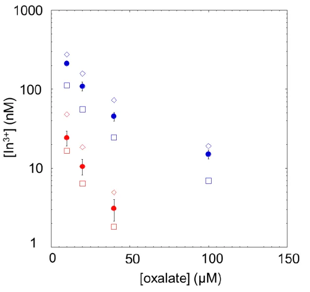
3.4 Speciation of indium with oxalate and humic acids 370

After establishing that the species measured by AGNES is indeed the free In3+, it is fundamental 371

to evaluate its performance in speciation studies. 372

Figure 6 shows that the results obtained in this study for In-oxalate binding are in reasonable 373

agreement with previously published results, since they lie halfway between the ones reported 374

by Pingarron et al [41] and the ones reported by Vasca et al [42]. In a previous work using 375

AGNES in the HMDE Tehrani et al [26] using somewhat different experimental conditions 376

observed values closer to the ones reported by Vasca et al [42]. We must warn that, because of 377

a typing error, the total concentration of indium of 100 mol L-1 was unduly reported as 5 mol 378

L-1 in the caption of figure 6 in [26]. 379

We estimated the errors for our AGNES measurements using the 95% confidence interval 380

obtained from the standard deviation of the 4 measurements multiplied by Student factor for 381

binomial distributions (t95,3=3.182). As expected, the errors are larger for the smaller values

382

obtained at pH 4, since they are closer to the detection limit. 383

384

Figure 6: Free indium concentrations measured by AGNES in presence of increasing

385

concentrations of oxalate in 100 mM NaClO4 at pH 3 (blue circle) and pH 4 (red circle). Total

386

indium concentration is 0.1 µM. The rotation speed is 1000 rpm. Computed values using Visual 387

MinteQ with the stability constants determined by Pingarron et al [41] (open diamond) and 388

Vasca et al [42] (open square), and using the Biryuk et al [35] constants for the indium 389

hydroxides complexes. 390

391

One of our main interests in developing these methodologies is the ability to perform indium 392

speciation directly in environmental samples. Since the interaction of indium with natural 393

organic matter (NOM) is expected to be one of the key parameters, about which there is no 394

information in the literature, we decided to test AGNES in presence of a well-characterised 395

humic sample [31], as a representative colloidal phase in freshwaters. 396

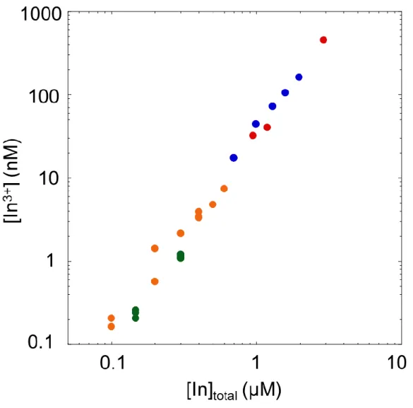
Figure 7 depicts an indium titration of 5 mg L-1 of humic acid substance, at pH 3.75, 100 mM 397

NaClO4, i.e., the free indium evolution as a function of the total indium concentration added.

The orange and green points at very low indiumconcentration were obtained using the strategy 399

of changing the deposition potential and computing the new gain using Eq. (3.3). In this 400

particular case the calibration linked Ecalib = 0.5800V with Ycalib = 1.6×104, and the new gain

401

for the experiment in presence of humic acids at Ed = 0.6300V was Y = 3.3×106. In this way,

402

four decades of free indium concentrations are probed by the AGNES technique with 403

reasonable equilibrium times (less than 10 min). Thus, this methodology opens the way to the 404

elaboration of indium binding isotherms over a wide range of metal coverage to humic acid 405

particles. Moreover, we observe a reasonable repeatability amongst the different measurement 406

(replicates) demonstrating the ability of AGNES to provide robust speciation data. 407

408

Figure 7: Free indium concentrations measured by AGNES in several suspensions of humic acids (5

409

mg L-1_{) containing known total indium concentrations, at pH 3.75 and ionic strength of 100 mM NaClO} 4. 410

The rotation speed is 1000 rpm. Each colour corresponds to replicates. Error bars estimated from the

411

relative uncertainties over three AGNES measurements, are smaller than points.

412 413 414

Conclusions

415

In this work we investigated the ability of two electroanalytical techniques to measure low 416

concentration of total (SCP) and free indium (AGNES). For the total concentration, at pH <2.3, 417

we obtained an excellent detection limit of 0.5 nM for 180 s deposition time. 418

For the free metal determination using AGNES, we demonstrated the enormous saving in 419

experimental time when using the TMF/RDE instead of the HMDE and confirmed the excellent 420

performance of these electrodes in speciation studies, especially when determining extremely 421

low free indium concentrations (down to 10-10 _{M). We also verified that AGNES was able to}

422

provide robust speciation data in experiments in presence of humic matter. 423

Due to the absence of trivalent cation complexation data with humic matter, it is our intention 424

to pursue these studies with experiments at different pH values and different ionic strengths, 425

followed by adequate complexation modelling, especially at higher pH values where the 426

influence of indium hydrolysis will be noticeable. Such investigations will open new 427

perspectives for using indium as a powerful tracer of geochemical processes of trivalent 428

elements in terrestrial waters. 429

430

Acknowledgements

431

This work has been supported by the French National Research Agency through the national 432

program “Investissements d’avenir” with the reference ANR-10-LABX-21-01 / LABEX 433

RESSOURCES21. We thank the contribution of Jérémy Gloux, Paco Iglesias and Mirella 434

Dammous from University of Lorraine in the preliminary experimental work. Funding from the 435

Spanish Ministry of Economy, Industry and Competitiveness MINECO, project CTM2016-436

78798 (EC, PPV, JG) is acknowledged. PPV thanks Generalitat de Catalunya for a doctoral FI-437 AGAUR fellowship. 438 439 Supplementary material 440

Section 1: Linearity range for In3+ _{in SCP with TMF/RDE.}

441

Section 2: Stripping Chronopotentiometry (SCP) at the TMF/RDE. 442

Section 3: Fundamentals of AGNES. 443

Section 4: Calibration plots obtained with AGNES. 444 445 AUTHOR INFORMATION 446 Corresponding Author 447 *Email: [email protected] 448 449 References 450

[1] European Commission, Critical Metals in the Path towards the Decarbonisation of the EU 451

Energy Sector: Assessing Rare Metals as Supply-Chain Bottlenecks in Low-Carbon 452

Energy Technologies, (2013). https://ec.europa.eu/jrc/en/publication/eur-scientific-and-453

technical-research-reports/critical-metals-path-towards-decarbonisation-eu-energy-454

sector-assessing-rare-metals-supply. 455

[2] U.S. Geological Survey, 2017, Mineral commodity summaries 2017, (2017). 456

https://doi.org/10.3133/70180197. 457

[3] L. Ciacci, B.K. Reck, N.T. Nassar, T.E. Graedel, Lost by Design, Environ. Sci. Technol. 458

49 (2015) 9443–9451. doi:10.1021/es505515z. 459

[4] S.J.O. White, H.F. Hemond, The Anthrobiogeochemical Cycle of Indium: A Review of 460

the Natural and Anthropogenic Cycling of Indium in the Environment, Crit. Rev. Environ. 461

Sci. Technol. 42 (2012) 155–186. doi:10.1080/10643389.2010.498755. 462

[5] Y. Nozaki, D. Lerche, D.S. Alibo, M. Tsutsumi, Dissolved indium and rare earth elements 463

in three Japanese rivers and Tokyo Bay: Evidence for anthropogenic Gd and In, Geochim. 464

Cosmochim. Acta. 64 (2000) 3975–3982. doi:10.1016/S0016-7037(00)00472-5. 465

[6] A. Tessier, C. Gobeil, L. Laforte, Reaction rates, depositional history and sources of 466

indium in sediments from Appalachian and Canadian Shield lakes, Geochim. Cosmochim. 467

Acta. 137 (2014) 48–63. doi:10.1016/j.gca.2014.03.042. 468

[7] H.-W. Chen, Gallium, Indium, and Arsenic Pollution of Groundwater from a 469

Semiconductor Manufacturing Area of Taiwan, Bull. Environ. Contam. Toxicol. 77 470

(2006) 289–296. doi:10.1007/s00128-006-1062-3. 471

[8] S.J.O. White, F.A. Hussain, H.F. Hemond, S.A. Sacco, J.P. Shine, R.L. Runkel, K. 472

Walton-Day, B.A. Kimball, The precipitation of indium at elevated pH in a stream 473

influenced by acid mine drainage, Sci. Total Environ. 574 (2017) 1484–1491. 474

doi:10.1016/j.scitotenv.2016.08.136. 475

[9] A. Ladenberger, A. Demetriades, C. Reimann, M. Birke, M. Sadeghi, J. Uhlback, M. 476

Andersson, E. Jonsson, GEMAS: Indium in agricultural and grazing land soil of Europe - 477

Its source and geochemical distribution patterns, J. Geochem. Explor. 154 (2015) 61–80. 478

doi:10.1016/j.gexplo.2014.11.020. 479

[10] K. Folens, G. Du Laing, Dispersion and solubility of In, Tl, Ta and Nb in the aquatic 480

environment and intertidal sediments of the Scheldt estuary (Flanders, Belgium), 481

Chemosphere. 183 (2017) 401–409. doi:10.1016/j.chemosphere.2017.05.076. 482

[11] N.R. Brun, V. Christen, G. Furrer, K. Fent, Indium and Indium Tin Oxide Induce 483

Endoplasmic Reticulum Stress and Oxidative Stress in Zebrafish (Danio rerio), Environ. 484

Sci. Technol. 48 (2014) 11679–11687. doi:10.1021/es5034876. 485

[12] C. Zeng, A. Gonzalez-Alvarez, E. Orenstein, J.A. Field, F. Shadman, R. Sierra-Alvarez, 486

Ecotoxicity assessment of ionic As(III), As(V), In(III) and Ga(III) species potentially 487

released from novel III-V semiconductor materials, Ecotoxicol. Environ. Saf. 140 (2017) 488

30–36. doi:10.1016/j.ecoenv.2017.02.029. 489

[13] C.I. Olivares, J.A. Field, M. Simonich, R.L. Tanguay, R. Sierra-Alvarez, Arsenic (III, V), 490

indium (III), and gallium (III) toxicity to zebrafish embryos using a high-throughput multi-491

endpoint in vivo developmental and behavioral assay, Chemosphere. 148 (2016) 361–368. 492

doi:10.1016/j.chemosphere.2016.01.050. 493

[14] S.A. Wood, I.M. Samson, The aqueous geochemistry of gallium, germanium, indium and 494

scandium, Ore Geol. Rev. 28 (2006) 57–102. doi:10.1016/j.oregeorev.2003.06.002. 495

[15] A. Tessier, C. Gobeil, L. Laforte, Reaction rates, depositional history and sources of 496

indium in sediments from Appalachian and Canadian Shield lakes, Geochim. Cosmochim. 497

Acta. 137 (2014) 48–63. doi:10.1016/j.gca.2014.03.042. 498

[16] V.K. Gupta, A.J. Hamdan, M.K. Pal, Comparative study on 2-amino-1,4-naphthoquinone 499

derived ligands as indium (III) selective PVC-based sensors, Talanta. 82 (2010) 44–50. 500

doi:10.1016/j.talanta.2010.03.055. 501

[17] M.N. Abbas, H.S. Amer, A Solid-Contact Indium(III) Sensor based on a Thiosulfinate 502

Ionophore Derived from Omeprazole, Bull. Korean Chem. Soc. 34 (2013) 1153–1159. 503

doi:10.5012/bkcs.2013.34.4.1153. 504

[18] C. Pérez-Ràfols, N. Serrano, J.M. Díaz-Cruz, C. Ariño, M. Esteban, Simultaneous 505

determination of Tl(I) and In(III) using a voltammetric sensor array, Sens. Actuators B 506

Chem. 245 (2017) 18–24. doi:10.1016/j.snb.2017.01.089. 507

[19] J. Zhang, Y. Shan, J. Ma, L. Xie, X. Du, Simultaneous Determination of Indium and 508

Thallium Ions by Anodic Stripping Voltammetry Using Antimony Film Electrode, Sens. 509

Lett. 7 (2009) 605–608. doi:10.1166/sl.2009.1117. 510

[20] H. Sopha, L. Baldrianova, E. Tesarova, S.B. Hocevar, I. Svancara, B. Ogorevc, K. Vytras, 511

Insights into the simultaneous chronopotentiometric stripping measurement of 512

indium(III), thallium(I) and zinc(II) in acidic medium at the in situ prepared antimony film 513

carbon paste electrode, Electrochimica Acta. 55 (2010) 7929–7933.

514

doi:10.1016/j.electacta.2009.12.089. 515

[21] I. Geca, M. Korolczuk, Sensitive Anodic Stripping Voltammetric Determination of 516

Indium(III) Traces Following Double Deposition and Stripping Steps, J. Electrochem. 517

Soc. 164 (2017) H183–H187. doi:10.1149/2.0581704jes. 518

[22] K.C. Honeychurch, Recent Developments in the Stripping Voltammetric Determination 519

of Indium, World J. Anal. Chem. World J. Anal. Chem. 1 (2013) 8–13. doi:10.12691/wjac-520

1-1-2. 521

[23] J. Galceran, E. Companys, J. Puy, J. Cecilia, J.L. Garces, AGNES: a new electroanalytical 522

technique for measuring free metal ion concentration, J. Electroanal. Chem. 566 (2004) 523

95–109. doi:10.1016/j.jelechem.2003.11.017. 524

[24] R.F. Domingos, C. Huidobro, E. Companys, J. Galceran, J. Puy, J.P. Pinheiro, Comparison 525

of AGNES (absence of gradients and Nernstian equilibrium stripping) and SSCP (scanned 526

stripping chronopotentiometry) for trace metal speciation analysis, J. Electroanal. Chem. 527

617 (2008) 141–148. doi:10.1016/j.jelechem.2008.02.002. 528

[25] L.S. Rocha, E. Companys, J. Galceran, H.M. Carapuça, J.P. Pinheiro, Evaluation of thin 529

mercury film rotating disk electrode to perform absence of gradients and Nernstian 530

equilibrium stripping (AGNES) measurements, Talanta. 80 (2010) 1881–1887. 531

doi:10.1016/j.talanta.2009.10.038. 532

[26] M.H. Tehrani, E. Companys, A. Dago, J. Puy, J. Galceran, Free indium concentration 533

determined with AGNES, Sci. Total Environ. 612 (2018) 269–275.

534

doi:10.1016/j.scitotenv.2017.08.200. 535

[27] N. Serrano, J.M. Díaz‐Cruz, C. Ariño, M. Esteban, Stripping Chronopotentiometry in 536

Environmental Analysis, Electroanalysis. 19 (2007) 2039–2049.

537

doi:10.1002/elan.200703956. 538

[28] R.M. Town, H.P. van Leeuwen, Effects of adsorption in stripping chronopotentiometric 539

metal speciation analysis, J. Electroanal. Chem. 523 (2002) 1–15. doi:10.1016/S0022-540

0728(02)00747-7. 541

[29] E. Companys, J. Galceran, J.P. Pinheiro, J. Puy, P. Salaün, A review on electrochemical 542

methods for trace metal speciation in environmental media, Curr. Opin. Electrochem. 3 543

(2017) 144–162. doi:10.1016/j.coelec.2017.09.007. 544

[30] E.M. Thurman, R.L. Malcolm, Preparative isolation of aquatic humic substances, Environ. 545

Sci. Technol. 15 (1981) 463–466. doi:10.1021/es00086a012. 546

[31] W.G. Botero, M. Pineau, N. Janot, R.F. Domingos, J. Mariano, L.S. Rocha, J.E. 547

Groenenberg, M.F. Benedetti, J.P. Pinheiro, Isolation and purification treatments change 548

the metal-binding properties of humic acids: effect of HF/HCl treatment, Environ. Chem. 549

14 (2018) 417–424. doi:10.1071/EN17129. 550

[32] S.C.C. Monterroso, H.M. Carapuca, J.E.J. Simao, A.C. Duarte, Optimisation of mercury 551

film deposition on glassy carbon electrodes: evaluation of the combined effects of pH, 552

thiocyanate ion and deposition potential, Anal. Chim. Acta. 503 (2004) 203–212. 553

doi:10.1016/j.aca.2003.10.034. 554

[33] C. Parat, L. Authier, D. Aguilar, E. Companys, J. Puy, J. Galceran, M. Potin-Gautier, 555

Direct determination of free metal concentration by implementing stripping 556

chronopotentiometry as the second stage of AGNES, Analyst. 136 (2011) 4337–4343. 557

doi:10.1039/C1AN15481H. 558

[34] J.P. Gustafsson, Visual MINTEQ version 3.0. KTH, Department of Land and Water 559

Resources Engineering, Stockolm, Sweden, 2009. Available at http://vminteq.lwr.kth.se/, 560

(n.d.). 561

[35] E.A. Biryuk, V.A. Nazarenko, R.V. Ravitskaya, Spectrophotometric determination of the 562

hydrolysis constants of indium ions, Russian Journal of Inorganic Chemistry. 14 (1969) 563

503–506. 564

[36] W.W. Rudolph, D. Fischer, M.R. Tomney, C.C. Pye, Indium(III) hydration in aqueous 565

solutions of perchlorate, nitrate and sulfate. Raman and infrared spectroscopic studies and 566

ab-initio molecular orbital calculations of indium(III)–water clusters, Phys. Chem. Chem. 567

Phys. 6 (2004) 5145–5155. doi:10.1039/B407419J. 568

[37] F. Vydra, K. Štulík, E. Juláková, Electrochemical stripping analysis., E. Horwood, 569

Chichester, 1976. 570

[38] C. Huidobro, E. Companys, J. Puy, J. Galceran, J.P. Pinheiro, The use of microelectrodes 571

with AGNES, J. Electroanal. Chem. 606 (2007) 134–140.

572

doi:10.1016/j.jelechem.2007.06.001. 573

[39] E. Rotureau, Analysis of metal speciation dynamics in clay minerals dispersion by 574

stripping chronopotentiometry techniques, Colloids Surf. Physicochem. Eng. Asp. 441 575

(2014) 291–297. doi:10.1016/j.colsurfa.2013.09.006. 576

[40] R.R. Nazmutdinov, T.T. Zinkicheva, G.A. Tsirlina, Z.V. Kuz’minova, Why does the 577

hydrolysis of In(III) aquacomplexes make them electrochemically more active?, 578

Electrochimica Acta. 50 (2005) 4888–4896. doi:10.1016/j.electacta.2005.02.091. 579

[41] J.M. Pingarron, R. Gallego-Andreu, P. Sanchez-Batanero, Potentiometric determination 580

of stability constants of complexes formed by Indium(III) and different chelating agents, 581

Bull. Soc. Chim. Fr. 3–4 (1984) 115–122. 582

[42] E. Vasca, D. Ferri, C. Manfredi, L. Torello, C. Fontanella, T. Caruso, S. Orrù, Complex 583

formation equilibria in the binary Zn2+–oxalate and In3+–oxalate systems, Dalton Trans. 584

0 (2003) 2698–2703. doi:10.1039/B303202G. 585