DOCTORAT DE L'UNIVERSITÉ DE TOULOUSE
Délivré par :
Institut National Polytechnique de Toulouse (INP Toulouse)
Discipline ou spécialité :
Océan, Atmosphère et surfaces continentales
Présentée et soutenue par :
M. SILIANG LIU
le mercredi 11 juin 2014
Titre :
Unité de recherche :
Ecole doctorale :
IMPLEMENTATION OF A SATELLITE-BASED PROGNOSTIC DAILY
SURFACE ALBEDO DEPENDING ON SOIL WETNESS: IMPACT STUDY
IN SURFEX MODELLING PLATFORM OVER FRANCE
Sciences de l'Univers de l'Environnement et de l'Espace (SDUEE)
Centre National de Recherches Météorologiques (CNRM)
Directeur(s) de Thèse :
M. JEAN-LOUIS ROUJEAN
Rapporteurs :
Mme CRYSTAL BARKER SCHAAF, UNIVERSITY OF MASSACHUSSETS BOSTON M. SHUNLIN LIANG, UNIVERSITE DE MARYLAND
Membre(s) du jury :
1 M. FRANCK ROUX, UNIVERSITE TOULOUSE 3, Président
2 M. JEAN-LOUIS ROUJEAN, METEO FRANCE TOULOUSE, Membre
2 Mme DOMINIQUE COURAULT, INRA AVIGNON, Membre
Thèse préparée au sein du Laboratoire de Centre National de Recherches Météorologiques, Météo-France
Résumé
L’albédo de la surface est une variable clé en météorologie car elle assure le contrôle du rayon-nement solaire absorbé par la surface, et par là même elle régule le bilan d’énergie en surface. L’albédo est encore généralement prescrit à ce jour comme une grandeur climatologique organi-sée par classe d’occupation des sols afin de disposer d’atlas globaux spatialement cohérents. Une telle approche a fait son chemin alors que la télédétection propose maintenant des produits albé-dos fiables et fréquemment réactualisés, notamment réactifs à la chronologie des précipitations. C’est l’objet majeur de cette étude en cherchant à calibrer l’albédo de sol nu avec l’humidité superficielle et à mesurer l’impact sur les flux d’énergie.
La première étape de l’étude consiste à réaliser un état de l’art de la climatologie d’albédo de surface fondée sur les produits satellitaires, parmi quoi figure la base de données duale ECO-CLIMAP qui comprend une carte d’occupation des sols et des paramètres de surface associés. Une originalité de l’étude repose sur le développement d’une méthode pour obtenir un albédo MODIS journalier à 500m à partir du produit standard BRDF/Albédo à 8 jours et de la réflec-tivité mesurée lors du passage d’orbite de MODIS, ensuite renormalisé donc en albédo quotidien MODIS. Ce dernier est ensuite validé avec l’albédo similaire de l’instrument SEVIRI à bord du satellitaire géostationnaire MSG. Les 2 produits albédos montrent un bon accord général avec toutefois des différences en hiver, ce qui semble lié à la géométrie d’illumination, différente dans les 2 cas. Mais ces écarts restent faibles comparé à la climatologie actuelle de l’albédo considérée dans le schéma de surface ISBA-A-gs.
Dans les schémas de surface tel ISBA-A-gs, la séparation entre les albédos du sol nu et de la végétation permet de mieux prendre en compte des processus qui sont spatialement et temporel-lement indépendants. Alors que l’albédo de la végétation évolue plutôt sur une base saisonnière, celui du sol nu varie sur de courtes échelles de temps comme étant impacté par les événements de pluie générant une humidité superficielle. L’accumulation de séries pluri-annuelles de données MODIS a permis tout d’abord d’établir des albédos de sol nu et de végétation sur une base climatologique, pour être ensuite comparés, favorablement, avec leurs équivalents dans le modèle JULES du Met Office.
Un albédo de surface pronostique est ensuite mis en place pour les besoins du schéma de surface ISBA-A-gs en prenant en compte notamment l’humidité des sols et la chlorophylle des feuilles. Le volet humidité est cependant mieux consolidé grâce notamment à une calibration entre les albédos satellitaires de sol nu et l’humidité du sol mesurée en routine sur les 12 stations
SMOSMANIA du sud-ouest de la France. Le résultat est la prescription d’un albédo évolutif avec l’humidité bien corrélé avec les albédos satellitaires à l’échelle du paysage. Pour la composante végétation de l’albédo, l’étude repose sur des simulations du modèle détaillé de transfert radiatif PROSAIL. On en déduit des relations simplifiées entre l’albédo de la feuille et la chlorophylle, puis une nécessaire prise en compte de l’indice foliaire LAI lors du passage à l’échelle de la canopée végétale. L’albédo de la végétation ainsi obtenu combiné avec celui du sol nu permet de prescrire un albédo total, ce qui se vérifie bien avec les données de la station de Majadas (Espagne) situé dans l’écosystème naturel de grande échelle ‘dehesa’ et pour lequel humidité, chlorophylle et LAI sont continûment mesurés. Une fois consolidé la paramétrisation d’un albédo de surface pronostique, il est regardé les études d’impact de celui-ci par rapport à la climatologie. Pour cela, on considère le modèle SURFEX du bilan d’énergie sur la France et le forçage SAFRAN. Des simulations offline montrent des effets non négligeables sur la température et l’humidité à 2m ainsi que sur les flux (rayonnement net, chaleurs sensibles et latentes) pendant plusieurs jours en raison de la prise en compte d’un albédo réaliste qui soit moins sec. Dans une dernière étape, on a développé un schéma d’assimilation de l’albédo de type Simple Ensemble Kalman Filter (SEKF), ce qui a un effet sur le LAI simulé par ISBA-A-gs pour des végétations de densité faible à moyenne.
Abstract
Surface albedo is a key parameter in meteorology as it controls the absorbed solar radiation and besides regulates the surface energy balance. It is generally established as a climatologic value staged in land cover units to get trusting atlas. Such approach yields obviously some limits whe-reas today remote sensing observations offer a frequent update of surface albedo fields to be the echo of rainfall chronology. Owing to this, the surface albedo could be predicted from soil wetness. The first step of this study consists to review state-of-art satellite-based climatology of surface albedo, amongst which ECOCLIMAP-II, as it still popular for meteorology. The novelty relies on method development to get a a 500m daily surface albedo from LEO (low elevation orbit) MODIS 8 day BRDF/Albedo standard product renormalized to orbital pass reflectance. Daily MODIS surface albedo is further validated against LSA SAF product issued from geostationary (GEO) sensor SEVIRI data. LEO and GEO surface albedo show discrepancies over SMOSMA-NIA stations in winter and early spring periods in relation to the geometry of illumination. But more significant bias are conspicuous between satellite-based surface albedo products and the actual climatology used in ISBA-A-gs model. In land surface models, the partitioning of the surface albedo into soil and vegetation distinct albedo components allows to address different processes that are time-scale dependent. Vegetation albedo primarily varies along with the gro-wing season while soil albedo shows day-to-day variations caused by rainfall events. Multi-years MODIS accumulated observations are harnessed to firt stress a static unravelling between soil and vegetation serving for climatology. Resulting visible and near infrared albedos present assets in terms of completion and spatial consistency compared to equivalence in JULES model.
A prognostic surface albedo is further implemented for the purpose of ISBA-A-gs land sur-face model in accounting for (1) soil moisture and more preliminary on (2) leaf chlorophyll. Tests are carried on over the 12 SMOSMANIA anchor stations designed to measure routinely the soil moisture (SM) in south-western France for the cal/val SMOS. Using a physically-based parameterization between soil albedo and SM, forecast surface albedo matches well in time with LEO and GEO products. Besides, numerical simulations of vegetation canopies with PROSAIL radiative transfer model serve to derive a generic relationship between visible vegetation albedo and chlorophyll content (Cab), that is however constrained by the leaf area index (LAI). This relationship yields an update of vegetation albedo further combined with soil albedo to get a completion of the prognostic surface albedo. The approach is validated with in-situ measure-ments from ICOS station of Majadas (Spain) representative of the dehesa ecosystem.
Impact of changing surface albedo is accomplished using ISBA-A-gs over France running offline with SAFRAN as forcing. Through incorporating an ’albedo-soil moisture’ dependence in ISBA-A-gs, improvements are demonstrated for its modeling ability for energy balance. The energy fluxes (net radiation, sensible heat, latent heat) and surface temperature are revealing distinct seasonal and daily variations after introducing this soil wetness dependence of prognostic albedo.
Table des figures
1 Vue schématique des composantes du système climatique, de leurs processus et interactions. (Source from IPCC, 2007) . . . xx 2 Estimation du bilan d’énergie annuel et global de la Terre.(Source from Kiehl and
Trenberth, 1997) . . . xx 3 Résumé des principales composantes du forçage radiatif en lien avec le changement
climatique. La ligne horizontale rattachée à chaque couleur représente le rang d’incertitude pour la valeur respective. (Source from IPCC, 2007) . . . xxii 4 Skematic view of the components of the climate system, their processes and
inter-actions. (Source from IPCC, 2007) . . . xxvii 5 Estimate of the Earth’s annual and global mean energy balance. (Source from
Kiehl and Trenberth, 1997) . . . xxviii 6 Summary of the principal components of the radiative forcing of climate change.
The think black line attached to each color bar represents the range of uncertainty for the respective value. (Source from IPCC, 2007) . . . xxx 1.1 Sketch figure on the definitions of Black Sky Albedo, White Sky Albedo and Blue
Sky albedo. . . 2 1.2 Schematic representation of amplitude and duration of the sources of albedo
va-riations inferred from 7 years of MODIS and in situ data. (Sources from Samain et al., 2008) . . . 4 1.3 Global distribution of BSRN stations. Red dots denote BSRN stations which have
already submitted data offered in the WRMC. Green dots represent accepted BSRN stations which plan to submit data in future. BSRN stations which are closed are marked in blue. (Source from BSRN website http://www.bsrn.awi. de/.) . . . 9 1.4 Global distribution of the FLUXNET stations. (Source from website http://bwc.
berkeley.edu/Fluxnet-LaThuile/map/) . . . 10 1.5 Duration period of long-term available continental and global satellite albedo
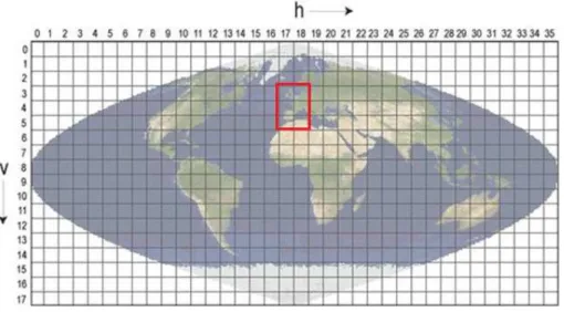
pro-ducts. . . 11 2.1 Tiles covering the study area in MODIS ISIN projection (red frame). . . 20 2.2 Processing chain of daily MODIS albedo. . . 23
2.3 Seasonal evolution of selected daily shortwave WSA over France in 2007 : (a)Julian Day 006-017, (b)Julian Day 186-197. Pixels influenced by cloud, snow, and
indi-cated with poor BRDF quality are rendered in grey color. . . 26
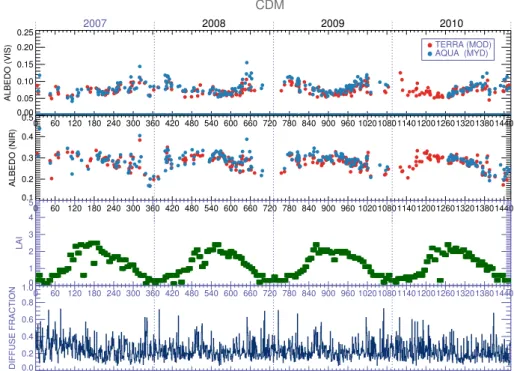
2.4 Time series of daily (a) MODIS WSA (VIS), (b) WSA (NIR), (c) LAI and (d) Diffuse Fraction during 2007-2010. Daily LAI is a linear interpolation from 8D MCD15A1 product. . . 27
2.5 Spatial distribution of 13 FLUXNET stations over France. (Noted : Lq1 and Lq2 are located in the same site, while the records begin at different time.) . . . 30
2.6 High resolution of GOOGLE MAPTM used to check the homogenity. Image co-vers an area of 1km2centre at the coordinate of the FLUXNET station.(a)Aurade, (b)Avignon, (c)Bilos, (d)Couhins, (e)Fontainbleu, (f)Grignon, (g)Hesse, (h)Lamsquerre, (i)Laqueuille, (j)LeBray, (k)Lusignan, (l)Peuchabon. . . 31
2.7 Time series comparison of TERRA/AQUA daily MODIS albedo with FLUXNET in 2007. . . 32
2.8 Diurnal variation of in-situ measured albedo at two FLUXNET stations : (a) Fontainebleau, (b) Le Bray comparing with daily MODIS albedo during Julian Day 110-120, 2007. . . 33
2.9 Scatter Plot of daily MODIS TERRA/AQUA albedo compared with FLUXNET measurements. Albedo retrievals from TERRA and AQUA are indicated in two different colors : orange and red, respectively. . . 33
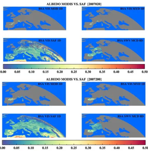
2.10 Comparison of Black Sky Albedo (BSA) between TERRA MODIS (MOD 1D), AQUA MODIS (MYD 1D), TERRA+AQUA MODIS (MCD 8D), SEVIRI (SAF 1D) on Julian Day 20 and 200 during 2007. . . 35
2.11 Density scatter plot of Black Sky Albedo (BSA) comparing MOD 1D, MYD 1D, MCD 8D, SAF 1D on (a) Julian Day 20 and (b) Julian Day 200 during 2007. . . 36
2.12 Seasonal evolution of MODIS and SEVIRI albedo products over four SMOSMA-NIA stations in 2007. . . 38
2.13 Composition of ECOCLIMAP database. . . 40
2.14 Scheme for aggregating parameters for mixed vegetation or soil types. . . 41
2.15 ECOCLIMAP II 273 ecosystem covers in Europe ((Faroux et al., 2013)) . . . 42
2.16 Comparison of three types of albedo : (a) ISBA model simulation, (b) MODIS MCD43B3, and (c) SAF L2 1-D albedo on two selected days : 2008/02/03 and 2008/08/03. . . 45
2.17 Difference of albedo : (a) MODIS-MODEL, and (b) SAF-MODEL on two selected days : 2008/02/03 and 2008/08/03. . . 46
2.18 Scatter plots of albedo on two selected days 2008/02/03 and 2008/08/03 : (a) MODIS-MODEL, and (b) SAF-MODEL. . . 47
3.1 Five components of radiation in our 2-stream model (a) rdd-reflectance : diffuse incoming->diffuse outgoing ; (b) tdd-transmittance : diffuse incoming->diffuse outgoing ; (c) rsd-reflectance : solar direction incoming->diffuse outgoing ; (d) tsd-transmittance : solar direction incoming-> diffuse outgoing ; (e) tss-tsd-transmittance : solar direction incoming-> solar direction outgoing. . . 53
3.3 Fraction of vegetation (fveg, red color), fraction of soil (fsoil, blue color) and their sum (orange color). Two cases are tested for VIS and NIR taking leaf single scatter reflectance as 0.09 and 0.35, respectively. . . 56 3.4 The fveg comparison : (1) fVEG from 2-stream model of SZA=0, (2) fVEG
from 2-stream model of SZA=30, (3) fVEG from 2-stream model of SZA=60, (4) fVEG=1-exp(-0.6LAI), (5) fVEG=1-exp(-0.5LAI). . . 57 3.5 Spectral response functions of MODIS and SEVIRI sensors. Typical spectral curves
of soil and green leaves are imposed as slash curves. . . 58 3.6 Sensitivity simulation of VIS and NIR albedo with rho and Rsoil. . . 58 3.7 Sensitivity test of VIS and NIR WSA with ALA under different configurations of
LAI and soil albedo. . . 59 3.8 Sensitivity test of VIS and NIR WSA with TAU under different configurations of
LAI and soil albedo. . . 59 3.9 Sensitivity test of VIS and NIR BSA with ALA under different configurations of
LAI and soil albedo. SZA is fixed as 45 degree. . . 60 3.10 Comparison of CNRM and SWANSEA global soil background albedo. Noted, the
VIS and NIR are using different legends. . . 63 3.11 Scatter plots of CNRM vs. SWANSEA global soil background albedo in VIS and
NIR ranges. . . 66 3.12 Rsoil and Wveg retrieval in two stations : CDM and URG. . . 68 3.13 Time series of MODIS total albedo is compared with the reconstructed total
al-bedo in two stations during a 4-year period of 2007-2010 : CDM and URG. In the upper panel, MODIS orginal 8-D time series (ORI) are plotted in orange color, reconstructed total albedo (REC) is shown in grey. In the middle panel, the resi-dual of (ORI-REC) is shown. In the lowest panel, in-situ soil moisture recorded from Theta-probe is plotted. . . 70 3.14 Rsoil and Wveg retrieval and associated goodness of fit in the box over the France. 71 3.15 Patches of ISBA over the box containing the France. . . 72 3.16 Leaf Single Scattering Reflectance (Wveg) analysis over (a) dominant PFTs and
(b) ecosystem in France. . . 72 3.17 Probability density functions for (a) ρvis (τvis) and (b) ρnir (τnir) as a priori
information. . . 74 3.18 Histogram of Wveg (Leaf Single Reflectance) within 4 ’pure’ PFTs for (a) VIS and
(b) NIR. . . 76 3.19 Histogram of Wveg (Leaf Single Reflectance) for ecosystem 325, 363. . . 77 3.20 Histogram of Rsoil (Soil Albedo) within soil units for (a) VIS and (b) NIR. . . . 78 3.21 Leaf reflectance ρ and background albedo R assimilation for Condom station in
(a) VIS broadband, and (b) NIR broadband. A priori and climatology information are marked as dashed straight lines in blue and black color, respectively. . . 79 3.22 Reconstructed WSA for (a) VIS and (b) NIR in Condom station. Original MCD43A3,
reconstruction from (1) Gradient method, (2) A priori information and (3) Clima-tology are also plotted for comparison. . . 80 3.23 Scatter plot of reconstructed albedo from Gradient method comparing with
4.1 The spatial distribution of SMOSMANIA stations. . . 88 4.2 (a) SVC Spectroradiometer for bare soil spectral sampling (b) ML3 Theta-Probe
for soil moisture measurements. . . 89 4.3 Different types of bare soil within 6 SMOSMANIA stations : (a)LZC, (b)SBR,
(c)SFL, (d)URG, (e)CDM, (f)CRD. . . 90 4.4 Bare soil spectral measured using SVC over 6 SMOSMANIA stations : (a)LZC,
(b)SBR, (c)SFL, (d)URG, (e)CDM, (f)CRD. . . 91 4.5 Spectral Response Function of four sensors : SEVIRI, MODIS, VEGETATION
and MERIS. . . 92 4.6 Soil line of bare soil albedo within 7 SMOSMANIA stations. . . 94 4.7 The dependence of surface soil albedo on moisture, calibrated at three stations :
(a)LHS (b)SBR and (c)URG. . . 95 4.7 Sensitivity test of reflectance and foliage chlorophyll content. . . 98 4.8 Sensitivity test of reflectance and leaf area index. . . 98 4.9 The relationship between reflectance SEVIRI B1 (0.6µm) and Cab calibrated using
PROSAIL, stratified by LAI. The variation range is caused by different configura-tions of other parameters are represented by black vertical bars, while the average dependence is marked by the straight curves. . . 100 4.10 Graph the relationship between TOC reflectance MERIS Band 5 (0.56µm) and
Cab calibrated using PROSAIL model and various LAI values. The same relation-ship at 510nm is shown for the sake of comparison. . . 100 4.11 Site map of Majadas extracted from GOOGLE MAP. . . 101 4.12 Seasonal variation of fraction of vegetation cover. . . 101 4.13 VIS albedo regressed against fraction of vegetation cover to separate soil albedo
and vegetation albedo. Two types of products are serving as inputs, namely MO-DIS (red circles) and BIOPAR(blue circles). . . 102 4.14 (a) Time series of various albedo products at 4km resolution : broadband VIS
black sky albedo of SEVIRI(black circles), BIOPAR(brown curves), spectral al-bedo at 560nm of MODIS(green curve). The in-situ surface soil moisture at -4cm is imposed (dark blue curve). (b) In-situ soil moisture measurements at 4 layers : -4cm, -8cm, -10cm, -20cm, in reaction with local rainfall. (c) albedo calibrated with surface soil moisture (-4cm) using an exponential-like function. . . 103 4.15 (a) Seasonal variation of measured Cab (red circles), averaged measured Cab (blue
circles), and the quantity R560*sqrt(LAI) using MODIS reflectance at 560nm and Biopar LAI (black circles) (b) R560*sqrt(LAI) against 1/Cab, the red points are in-situ measurement of Cab, where the dark blue line shows the regression using Eq. 4.1. . . 104 4.16 Relationship between total chlorophyll and nitrogen at Majadas anchor station
for tree leaves. . . 105 4.17 Yearly variations of observed and simulated albedo et Majadas station. Chronology
of rainfall events is shown for the sake of comparison with albedo products. Error bar represents uncertainty assessment for SEVIRI albedo in link to persistence information. . . 105 4.18 Phenology of the herbaceous layer in Majadas. . . 106
5.1 Impact assessement on (a)TALB, (b)WG1, (c)TG1, (d)RN, (e)H, (f)LE over
France. Scenario at 12 :00 UTC on Aug 1, 2007 is rendered as illustration. . . 111
5.2 Comparison of monthly average variations over France between the 2 scenarios (NEWS a REFE) regarding the impact on possible wet albedo on (a)TALB, (b)WG1, (c)TG1, (d)RN, (e)H, (f)LE. Time series of one year at 12 :00 UTC from Aug 1, 2007 to Jul 31, 2008 is shown. . . 114
5.3 Same as Fig. 5.2 but showing daily average instead of monthly average. . . 115
5.4 Diurnal variation of bare soil albedo impact on (a)TALB, (b)WG1, (c)TG1, (d)RN, (e)H, (f)LE in 10 days since Aug 1,2009. . . 118
5.5 Flow chart of ’propagation’ process during assimilation. . . 121
5.6 Comparison between the 4 experiments for LAI assimilation. . . 124
5.7 Same as Fig. 5.6 for SSM. . . 125
5.8 Same as Fig. 5.6 for DH_VI. . . 126
5.9 Same as Fig. 5.6 for DH_NI. . . 127
5.10 Same as Fig. 5.6 for DH_BB. . . 128
Liste des tableaux
1 Albédo de surface : résolution, précision et stabilité. . . xxi
2 Alb de surface : rlution, prsion et stabilit . . . xxix
1.1 Symbols and subscripts for albedo definition. . . 2
1.2 Albedo variation scale and driven factors for vegetation and soil . . . 6
1.3 Comparison of existing albedo products from satellites. . . 14
2.1 Spectral-to-Broadband Conversion coefifcients for MODIS (adopted from MOD09 ATBD) . . . 24
2.2 Site information of FLUXNET stations. Avalability during 2007-2010 is reported as ’*’. . . 29
2.4 Information of MODIS and SEVIRI albedo products . . . 34
2.5 ISBA vegetation patches used in ECOCLIMAP . . . 39
2.6 Vegetation albedo parameterization in ECOCLIMAP I . . . 43
3.1 The input variables of the 2-stream model. . . 52
3.2 The variation range of input variables to generate LUT. . . 67
3.3 2-stream retrieval Wveg, Rsoil and statistical scores for SMOSMANIA stations . 69 3.4 A priori information used for describing leaf single reflectance ρ and soil albedo r Gaussian probability distribution function. . . 73
4.1 Soil composition and vegetation types for SMOSMANIA stations. . . 87
4.2 Parameters and its variation range for PROSAIL model. . . 99
5.1 List of observed variables and associated errors. . . 122
5.2 Presentation of the four experimental scenarios for assimilation. . . 124
Table des matières
Résumé iii
Abstract v
Introduction Générale xix
General Introduction xxvii
1 Scientific Context 1
1.1 Physical Principle . . . 1
1.2 Environment Factors Driving Albedo Variation . . . 3
1.3 State-of-the-art albedo modeling in surface models . . . 6
1.4 Albedo Observations . . . 8
1.4.1 Site Measurements . . . 8
1.4.2 Satellite albedo products . . . 10
2 Observed and modeled surface albedo for NWP 17 2.1 Introduction . . . 17
2.2 Presentation of SEVIRI albedo product . . . 19
2.3 Construction of a Daily MODIS Albedo product . . . 19
2.3.1 Input data sets . . . 20
2.3.1.1 Geographic Domain and Input MODIS files . . . 20
2.3.1.2 Ancillary files . . . 21
2.3.2 Presentation of the Method . . . 21
2.3.2.1 Underlying physical assumptions and general description . . . . 21
2.3.2.2 Scaling BRDF shape . . . 22
2.3.2.3 Narrow to Broad Band conversion . . . 24
2.3.3 Calculate Sky Diffuse Fraction and Total Sky Albedo . . . 24
2.3.4 Results . . . 25
2.3.4.1 Examination of the input data . . . 25
2.3.4.2 Extracting time series over SMOSMANIA sites . . . 27
2.3.4.3 Validation with FLUXNET stations . . . 28
2.4 Intercomparison and validation of daily MODIS and SEVIRI albedo . . . 34
2.4.2 Comparison results . . . 34
2.5 ISBA albedo simulation state-of-art . . . 38
2.5.1 Patch Strategy . . . 38
2.5.2 Two versions of ECOCLIMAP database . . . 40
2.5.2.1 ECOCLIMAP I . . . 40
2.5.2.2 ECOCLIMAP II . . . 41
2.5.2.3 Albedo parameterization in ECOCLIMAP I . . . 41
2.5.2.4 Albedo parameterization in ECOCLIMAP II . . . 42
2.5.2.5 Differences between ECOCLIMAP I and ECOCLIMAP II vege-tation and soil albedo parameterization . . . 43
2.6 Comparison of ISBA simulation and daily MODIS/SEVIRI albedo . . . 44
2.7 Conclusion . . . 48
3 Separation between Soil and Vegetation Albedo 49 3.1 Introduction . . . 49
3.2 Physical justification of soil and vegetation separation . . . 50
3.2.1 A simple 2-stream model . . . 51
3.2.1.1 Physical Basis of Two-stream Scheme . . . 53
3.2.1.2 Fraction of vegetation cover . . . 54
3.2.2 Sensitivity test . . . 57
3.3 Static Soil and Vegetation Albedo Separation . . . 61
3.3.1 Existing Global Static Soil Maps . . . 61
3.3.1.1 SWANSEA soil background albedo . . . 61
3.3.1.2 CNRM soil background albedo . . . 61
3.3.1.3 Intercomparison of two Global Soil Albedo Maps . . . 62
3.3.2 2-Stream method based on SAIL . . . 66
3.3.2.1 Retrieval of Soil Albedo and Leaf Single Reflectance over France 66 3.3.2.2 Analysis of the results . . . 68
3.4 Dynamic Soil and Vegetation Albedo Separation . . . 73
3.4.1 A Priori Information . . . 73
3.4.1.1 A priori Information . . . 73
3.4.1.2 A priori information constrained within PFT, ecosystem, soil unit 73 3.4.2 Radiative Transfer Model for Dynamic Retrieval . . . 75
3.4.3 Application over SMOSMANIA stations . . . 75
3.5 Conclusion . . . 81
4 Construction of prognostic albedo 83 4.1 Introduction . . . 83
4.2 Calibration of Soil Surface Albedo with Soil Moisture . . . 84
4.2.1 Theoretical rationale . . . 84
4.2.2 Validation over SMOSMANIA stations . . . 86
4.2.2.1 Description of filed measurement sites and equipements . . . 86
4.2.2.2 Measurement method . . . 90
4.3 Calibration of Vegetation Albedo with Foliage Chlorophyll Content . . . 97
4.3.1 Introduction . . . 97
4.3.2 PROSAIL model and sensitivity experiment . . . 97
4.3.3 Calibration of reflectance with chlorophyll content . . . 99
4.4 In-situ Validation at Majadas . . . 100
4.4.1 Site information . . . 100
4.4.2 Separation of Aveg and Asoil . . . 101
4.4.3 Variation of albedo with soil moisture . . . 102
4.4.4 Calibration of Aveg with Cab . . . 104
4.5 Conclusion . . . 107
5 Implementation in SURFEX 109 5.1 Introduction . . . 109
5.2 Impact of changing albedo . . . 110
5.2.1 Description of experiment . . . 110
5.2.2 Results of changing albedo on energy flux components . . . 111
5.2.2.1 Spatial distribution over France . . . 111
5.2.2.2 Seasonal and Daily Variation . . . 113
5.2.2.3 Diurnal variation . . . 117
5.3 Joint Assimilation of LAI, SSM and albedo . . . 120
5.3.1 Study station, model and observations . . . 120
5.3.2 Data Assimilation Scheme and Experiment setup . . . 120
5.3.3 Results . . . 123
5.4 Conclusion . . . 130
6 Conclusion and Prospectives 131
7 Conclusion et Perspectives 133
Acronyms 135
Bibliographie 141
Annexes 153
A A parameterization of SEVIRI and MODIS daily surface albedo with soil
moisture : Calibration and validation over southwestern France 155
B Processing of the input directional reflectance and BRDF products 173
Introduction Générale
Le changement climatique global est devenu l’un des plus importants centres d’intérêt scien-tifique et politique en matière de débat. Il existe plusieurs signes avant-coureurs à l’origine de la causalité du changement climatique, tel l’augmentation de la concentration des gaz à effet de serre, les aléas extrêmes, l’augmentation de la température, l’accroissement des précipita-tions, l’acidification des océans, la hausse du niveau des mers, le retrait des glaces, etc (Stocker et al., 2013). Ces constats avérés ont gagné la reconnaissance du public et influencé les décisions politiques quelque peu, mais ont avant tout renforcé une collaboration internationale afin de dynamiser les études en science environnementales axées sur le système Terre.
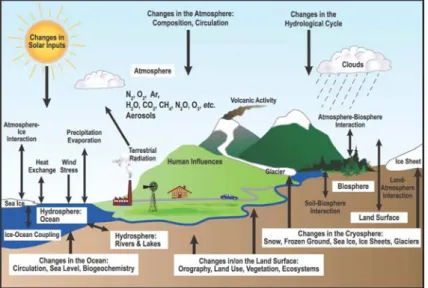
Le système Terre comprend plusieurs composantes ayant des frontières ténues : l’atmosphère, l’hydrosphère, la cryosphère, la biosphère et la géosphère. L’état de l’art des modèles représen-tant le fonctionnement du système Terre montre que ceux-ci peuvent représenter les processus pour chacune des composantes et simuler le stockage et les échanges de flux d’eau, d’énergie, et de matière biochimique entre les différents composants. En outre, les activités humaines, qui est l’un des facteurs les plus actifs et contrôlables, a de plus en plus d’influence sur le système clima-tique depuis l’ère industrielle. Comme montré en Fig.4, les différentes composantes du système Terre-atmosphère interagissent entre elles.
Les modèles de climat sont des outils puissants pour simuler la variabilité climatique consta-tée et pour faire des projections sur ce que pourrait être son état futur sous plusieurs scénarios de l’impact humain (Stocker et al., 2013). Les représentations des processus du système Terre se sont améliorées avec le temps en raison des ressources de calcul croissantes qui permettent de considérer des modèles ayant des résolutions de grille affinées. Ceci est particulièrement évident pour les composantes radiatives et les aérosols en liaison avec les interactions avec les nuages, aussi pour le traitement de la cryosphère. La représentation du cycle du carbone a été incorporée de façon extensive dans un grand nombre de modèles avec un effort significatif soutenu en matière de représentation depuis les conclusions du 4ième rapport d’évaluation de l’IPCC.
Le bilan d’énergie est l’une des composantes les plus importantes représentée dans les mo-dèles de climat étant donnée que le système climatique est piloté par le rayonnement solaire. Une carte schématique montre la contribution du rayonnement incident distribué entre les différentes composantes (fig.5). La réflectance de la planète Terre est approximativement 0.30, ce qui signifie qu’à peu près 30% de l’énergie rayonnée est rétro réfléchie vers l’espace. Le reste représente le rayonnement solaire incident rétro réfléchi vers l’atmosphère, les nuages, la surface, alors que la
Figure 1 – Vue schématique des composantes du système climatique, de leurs processus et interactions. (Source from IPCC, 2007)
part restante est absorbée par la surface ou l’atmosphère. Cette quantité représente approximati-vement 240 W/m2. Généralement, le rayonnement réchauffe la surface et refroidit l’atmosphère. L’énergie absorbée par la surface est retournée vers l’atmosphère sous forme de flux d’énergie sensible et latente. Pour équilibrer l’énergie incidente, la Terre elle-même émet du rayonnement infra-rouge, en moyenne d’une quantité équivalente à l’énergie dirigée en direction de l’espace.
Figure 2 – Estimation du bilan d’énergie annuel et global de la Terre.(Source from Kiehl and Trenberth, 1997)
Le flux d’énergie entre le soleil, la terre et l’espace relatif à l’équilibre radiatif Top of At-mosphere (TOA) peut être mesuré à partir du bilan radiatif réalisé par des missions tel CERES (Clouds and the Earth’s Radiant Energy System) (Wielicki et al., 1998) et Solar Radiation and
Table1 – Albédo de surface : résolution, précision et stabilité. Variable
para-meter
Horizontal Re-solution
Temporal Resolution Accuracy Stability
BSA 1KM Daily to Weekly max(5%,0.0025) max(1%,0.0001)
WSA 1KM Daily to Weekly max(5%,0.0025) max(1%,0.0001)
Climate Experiment (SORCE) (Kopp et al., 2005), respectivement. Les composantes du bilan radiatif à la surface sont plus difficiles à estimer de par le fait qu’elles ne peuvent être mesurées directement par satellite alors que les mesures en surface à partir de réseaux sol sont trop dis-persées pour être régionalement ou globalement représentatives. Des études récentes révèlent en global une atténuation et un éclaircissement, partant d’observations à long terme de photomètres solaires. Plusieurs études (Wild et al., 2008, 2004) ont indiqué un déclin dans le rayonnement net terrestre de l’ordre de 2W/m2 par décade entre 1960s et 1980s, et une augmentation du même taux entre 1980s et 2000. Ces constats sont fondés sur les échanges estimés des composantes radiatives individuelles qui constituent le rayonnement net à la surface :
Rn = (1 − α)Fds+ εFdl− σεTs4 = H + λE + G (1)
où apparaît le rayonnement descendant ondes-courtes Fs
d et thermique Fdl. L’albédo (α) et l’émissivité (ε) sont également 2 variables critiques déterminantes pour le rayonnement net, en optique et en thermique, respectivement, en considérant la constante de Planck σ et la tempéra-ture de peau T pour la seconde quantité. Le rayonnement net est équilibré par le flux de chaleur sensible (H), de chaleur latente (λE) et le terme de transport dans le sol (G).
Un suivi interprétable du climat de la Terre requiert des observations en routine de plusieurs paramètres atmosphériques, océaniques et terrestres. De fait, cela doit répondre à des technolo-gies combinées, depuis des instruments basés au sol à des bateaux, bouées, profileurs océaniques, ballons, avions, instruments embarqués, etc.. Global Climate Observing System (GCOS, 2009) a défini une liste de 50 Variables Climatiques Essentielles (ECV en anglais), qui sont techni-quement et économitechni-quement possiblement observables, afin de supporter le travail des United Nations Framework Convention on Climate Change(UNFCCC) et de l’IPCC. Parmi les ECV terrestres, l’albédo de surface en est une de particulièrement critique pour le bilan d’énergie dans le spectre solaire. Les résolutions temporelles et spatiales de l’albédo de surface et ses précision et stabilité attendues sont listées dans la Table 2.
Les changements dans l’atmosphère, la surface émergée, l’océan, la biosphère et la cryosphère – à la fois naturels et anthropiques - peuvent perturber le bilan radiatif de la Terre, et pro-duire un forçage radiatif (RF) qui affecte le climat. RF est une mesure du changement net du bilan d’énergie en réponse à une perturbation externe. Tous ces forçages radiatifs issus d’un ou de plusieurs facteurs affectant le climat et comme étant associés avec l’activité humaine ou les processus naturels sont discutés ici. L’albédo de surface est listé comme étant une variable ECV en lien avec le changement climatique qui soit possiblement encore quelque peu erronée et qui doit définitivement gagner en précision. Fig.6 montre les rangs de variation du forçage
radiatif moyen et leur incertitude pour les différents termes, parmi lesquels l’albédo indique un effet double. Selon les estimations faites entre 1750 et 2005 par le Intergovernmental Panel on Climate (IPCC), le changement sur l’albédo de surface causé par l’occupation des sols est estimé avoir un forçage négatif (refroidissement), de l’ordre de -0.2±0.2W/m2; et un forçage positif (réchauffement) causé par le dépôt de carbone suie sur la neige, de l’ordre de 0.1±0.1W/m2.
Figure 3 – Résumé des principales composantes du forçage radiatif en lien avec le changement climatique. La ligne horizontale rattachée à chaque couleur représente le rang d’incertitude pour la valeur respective. (Source from IPCC, 2007)
Les rétroactions de l’albédo de surface sur le climat et le cycle du carbone ont fait l’objet de nombreuses études. A ce propos, la région du Sahel a été un premier exemple mis en exergue du-rant la sécheresse sévissant dans la période 1970s-1980s (Charney et al., 1977). Un autre exemple de rétroaction positive typique existe avec l’albédo de la neige sur le système climatique pour les régions les plus septentrionales (Fletcher et al., 2009). En outre, la forêt Amazonienne a aussi été le centre d’intérêt de nombreuses études. De manière générale, il est maintenant largement reconnu que les mécanismes dus à un accroissement des valeurs d’ albédo soit dues à la désertifi-cation ou la déforestation résultent en une réduction des précipitations et de l’évapotranspiration (Dirmeyer and Shukla, 1994; Lofgren, 1995; Xue, 1996; Xue and Shukla, 1993). La déforestation boréale due à une baisse de l’albédo de surface a montré un biais pour les puits de carbone potentiels (Betts, 2000). Cependant, l’effet de refroidissement inhérent à un bond de l’ albédo de surface est possiblement compensé par un scénario de réchauffement résultant d’une évapo-transpiration significativement réduite. Le manque d’accord entre les résultants de modèle est en partie du à des différences entre les formulations des schémas de surface et de leurs champs de
paramètres, en dehors du fait que les mécanismes d’interaction surface-atmosphère ne sont pas entièrement maîtrisés.
La surface terrestre est une composante en soit du système Terre et aussi une composante interactive avec l’atmosphère et l’océan. Les modèles de surface (LSM en anglais) ont été originel-lement développés pour simuler grossièrement les échanges d’énergie, de matière et de moments vers l’atmosphère. De nos jours, le degré de sophistication des LSM a considérablement évolué pour répondre aux besoins des simulations climatiques. Dans la revue qui en a été faite de ces modèles par (Sellers et al., 1997), les LSM ont suivi 3 stades de développement :
(1) Le premier, opéré entre 1960 et 1970, était basé simplement sur les formules de transfert aérodynamique pour un bloc avec le plus souvent une prescription uniforme de paramètres de surface (albédo, rugosité aérodynamique, et disponibilité en humidité du sol).
(2) Dans les années 1980s, une seconde génération de modèles ont explicitement reconnu les effets de la végétation dans le calcul du bilan d’énergie à la surface. Les paramètres des propriétés de la surface furent assemblés selon des considérations écologiques et géographiques disponibles dans la littérature scientifique.
(3) La troisième génération de modèles utilise des théories modernes sur la photosynthèse et sa relation avec l’eau des plantes afin de fournir une description consistante du transfert d’énergie, de l’évapotranspiration, et des échanges de carbone par les plantes. Une série d’expériences de grand échelle ont pu être réalisées pour valider les processus des modèles et les hypothèses de changement d’échelle induites dans les schémas surface-atmosphère. Ces expériences ont aussi accéléré le développement de méthodes pour assurer le transfert de données satellitaires dans des jeux de données globales de paramètres de surface au bénéfice des modèles.
Les processus de surface ont été pris en compte dans les modèles de climat via des para-métrisations qui vont de schémas simples à des représentations complexes. Les paramètres clé des modèles incluent notamment l’albédo, la fraction de végétation et la couverture de neige, la longueur de rugosité, la température de peau, et les propriétés du couvert végétal. Cependant, ces variables ont été représentées de façon crue avec le temps en raison des capacités limitées d’observation. Mais la génération actuelle des satellites peut maintenant fournir le degré souhai-table d’information en terme d’échantillonnage spatial global à des intervalles de temps réguliers. Ainsi, la télédétection a clairement atteint un niveau de capacité suffisant pour estimer avec pré-cision maintenant les paramètres de surface de façon systématique, comme requis. D’un autre côté, la disponibilité des données d’observation des satellites a motivé les modélisateurs avides d’améliorer leur représentation des interactions entre le sol, la végétation, et l’atmosphère avec quelques différences sensibles mises en lumière dans le cadre de l’initiative PILPS (the Intercom-parison of Land-surface Parameterization Schemes).
Dans la droite ligne de PILPS, comme étant un ‘open-access’ et une activité pérenne, RA-diation transfer Model Intercomparison (RAMI) a opéré des phases successives. Chacune de ces phases cherche à redéfinir la capacité, la performance et l’accord de la dernière génération de modèles de transfert radiatif (RT). Ceci peut conduire à des perfectionnements de modèle et plus loin à des développements au bénéfice de la communauté modélisatrice en charge du transfert radiatif. Les modèles sont comparés à différents scénarios avec des densités de végétation
diffé-rentes, ce qui vaut aussi pour le LAI, le sol, etc. Depuis la première phase de RAMI I en 1999, 4 phases ont été réalisées. La dernière, RAMI IV, constitue une comparaison prenant en compte un modèle 3D de Monte Carlo comme référence. Le détail d’information peut être retrouvé sous http://rami-benchmark.jrc.ec.europa.eu/HTML/. Cependant, RAMI est axé sur des couverts thématiquement homogènes avec pour objectif de guider le développement de modèles de trans-fert radiatif. Cela ne peut servir pour valider les modèles de TR à la résolution de grille lâche du pixel d’un instrument satellitaire où des attributs complexes de la surface se trouvent être mélangés.
Avec la nouvelle génération de satellites d’observation de la Terre durant les 2 dernières dé-cades, des jeux variés d’albédos de surface à l’échelle globale et continentale ont été constitués. Cela concerne les instruments à orbite polaire tel MODIS (Moderate Resolution Imaging Spectro-radiometer), POLDER (Polarization and Directionality of Earth Reflectance) et VEGETATION embarqué sur SPOT, aussi les systèmes géostationnaires d’observation tel SEVIRI (Spinning Enhanced Visible and InfraRed Imager) sur METEOSAT Second Generation (MSG). Ces don-nées enregistrées sont dérivées de réflectance bien calibrées grâce à l’utilisation de chaînes de traitement élaborées et à des algorithmes physiques mieux consolidés. Les communautés climat et aussi prévision du temps sensible avancent régulièrement qu’une précision de l’ordre de 2-5% est requise pour un albédo de surface observé utilisable dans la modélisation de la surface. (se-lon le GCOS) Plusieurs exercices de validation (exemple du LPV/CEOS) ont confirmé la bonne précision obtenue avec les produits satellitaires récents, i.e. MODIS (Jin, 2003). Cela suppose davantage d’efforts pour raffiner la description de l’albédo de surface dans les modèles d’interface (Oleson, 2003). L’accumulation de jeux d’ observations consistants sur le long terme, typique-ment sur une base pluriannuelle, est jugée prometteuse pour servir à établir une climatologie des albédos du sol et de la végétation. Récemment une carte statique globale de l’albédo du sol nu a été proposée par (Houldcroft et al., 2009) en exploitant des séries pluriannuelles de données MODIS. Mais les variations à court terme de l’albédo du sol nu, principalement pilotées par l’humidité de surface (SSM en anglais) ne furent pas explorées. En fait, un examen quotidien de l’albédo de surface est au minimum requis afin d’évaluer l’humidité superficielle du sol. Il s’agit là véritablement d’un challenge pour les instruments à orbite polaire tel MODIS étant donné qu’avec une simple revisite quotidienne, toute information potentiellement réactualisable peut être sévèrement occultée par une haute fréquence d’ennuagement pour certaines régions. D’un autre côté, une analyse soignée des variations à court-terme de l’albédo de surface est réalisable avec les satellites géostationnaires mais pour des zones limitées du globe. Cependant les sys-tèmes d’observation LEO (low elevation orbit) peuvent toujours offrir des résolutions spatiales et spectrales améliorées comparées aux satellites GEO (geostationnary). De fait, une combinai-son entre LEO et GEO paraît opportune, ce qui passe nécessairement par des études séparées pour commencer. En sus d’un produit humidité du sol SSM, les aléas climatiques (inondations, orages, vents violents) peuvent être à la base de variations à court terme de l’albédo de surface du fait qu’ils alimentent et modulent la chronologie des épisodes de chute de pluie, de neige et des périodes alternées de croissance et de sénescence pour la végétation.
Dans les modèles de type SVAT, on considère une séparation entre la végétation et le sol nu car ces 2 entités font référence à différentes propriétés prises en compte dans différents processus
relativement au rayonnement solaire, à la chaleur, et au transfert hydrique. L’albédo de la végé-tation peut varier à des échelles de temps journalières et semainales en phase avec la variation de croissance des feuilles, du déplacement du contenu en chlorophylle, des pigments bruns ou même du contenu en eau des feuilles, tout cela dépendant plus ou moins de la longueur d’onde. D’un autre côté, l’albédo d’un sol nu va plutôt varier sur une base horaire car le champ principal de perturbation est l’humidité SSM liée aux précipitations. La modélisation des variations saison-nières de l’albédo de la végétation est primordiale pour réaliser des estimations quantitatives du changement de l’écosystème. Au lieu de cela, de rapides variations causées sur l’albédo du sol nu seront connectées avec la chronologie de la pluie, ce qui doit forcément être pris en compte dans la recherche de fermeture du bilan d’énergie.
Bien que plusieurs objectifs soient balayés dans ce travail de thèse, on peut résumer l’étude en se focalisant simplement sur les points suivants : (1) en premier lieu la mise en oeuvre d’un albédo de surface pronostique dans ISBA fondée sur un étalonnage des données de satellites LEO et GEO avec des données d’humidité SSM mesurées in-situ, et pour un cas pilote avec la chlorophylle ; (2) ensuite il est évalué l’impact d’un changement de l’albédo de surface du à l’humidité dans le bilan d’énergie de la plate-forme de développement SURFEX sur la France ; (3) en dernier lieu, on montre pour la première fois une assimilation de l’albédo de surface conjointement avec l’indice folaire LAI et l’humidité pour une station pilote de référence.
General Introduction
Global climate change has becoming one of the most important scientific and political topics. Many indicators have implied climate change, as green house gas concentration augmentation, extreme events, surface temperature rising, precipitation change, ocean acidification, sea level rise, glacial retreat, etc (Stocker et al., 2013). These findings gained the public recognition, in-fluenced political decision, enhanced the international cooperation, and boosted the study of earth system science.
Earth system has various components : atmosphere, hydrosphere, cryosphere, biosphere and geosphere. State-of-the-art Earth System Models (ESMs) can represent the processes within each components and simulate the storage and exchange fluxes of water, energy, and biochemistry mat-ter between different components. Further, the human activities, which is one of the most active and controllable factor, has more and more influence to the climate system since industry era. As shown in Fig.4, various components in the Earth-atmosphere system interact with each other.
Figure 4 – Skematic view of the components of the climate system, their processes and inter-actions. (Source from IPCC, 2007)
Climate models are used to simulate climate variability and to project the future status under various scenarios of human impact (Stocker et al., 2013). The horizontal and vertical resolution is augmenting. Representations of Earth system processes are much more extensive and improved, particularly for the radiation and the aerosol cloud interactions and for the treatment of the cryosphere. The representation of the carbon cycle was added to a larger number of models and has been improved since IPCC 4th Assessment Report.
Energy balance is one of the most important components represented by climate models since the climate system is driven by solar radiation. A sketch map shows the participation of inco-ming radiation distributed between different components (fig.5). The Earth’s planet reflectance is approximate 0.30, meaning that nearly 30% energy is reflected back to the space. Incoming solar radiation is reflected back by atmosphere, cloud, and surface, while the remaining part is absorbed by surface or atmosphere. The energy that is not reflected back to space is absorbed by the Earth’s surface and atmosphere. This amount is approximately 240 Watts per squaremetre (W/m2). Generally, the radiation warms the surface and cools the atmosphere. The absorbed energy of surface is returning back through atmosphere as sensible and latent heat fluxes. To balance the incoming energy, the Earth itself radiate through longwave radiation, on average, the same amount of energy back to space.
Figure5 – Estimate of the Earth’s annual and global mean energy balance. (Source from Kiehl and Trenberth, 1997)
The energy flux between Sun, Earth, and Space relative to Top of Atmosphere (TOA) ra-diation balance can be measured from CERES (Clouds and the Earth’s Radiant Energy Sys-tem) (Wielicki et al., 1998) and the Solar Radiation and Climate Experiment (SORCE), (Kopp et al., 2005), respectively. While the components of the radiation budget at the surface are more difficult to estimate since they can not be measured by satellite directly and the sur-face measurements are not regionally or globally representative. Recent studies reveal the global ’dimming’ and ’brightening’ from long-term sun-photometer observations. Wild et al. (2008, 2004) inferred a decline in land surface net radiation on the order of 2W/m2 per decade from
Table2 – Alb de surface : rlution, prsion et stabilit Variable
para-meter
Horizontal Re-solution
Temporal Resolution Accuracy Stability
BSA 1KM Daily to Weekly max(5%,0.0025) max(1%,0.0001)
WSA 1KM Daily to Weekly max(5%,0.0025) max(1%,0.0001)
the 1960s to the 1980s, and an increase at a similar rate from the 1980s to 2000, based on estimated changes of the individual radiative components that constitute the surface net radia-tion.
Rn = (1 − α)Fds+ εFdl− σεTs4 = H + λE + G (2)
Surface net radiation can be expressed as the combination of downward shortwave radiation Fds and longwave radiation Fdl . Albedo and emissivity are two critical variables determining the net radiation, in shortwave and thermal range, respectively. This net radiation is balanced by sensible heat (H), latent heat (λE) and ground transportation (G).
Improved understanding and systematic monitoring of Earth’s climate requires observations of various atmospheric, oceanic and terrestrial parameters and therefore has to reply on various technologies (ranging from ground-based instruments to ships, buoys, ocean profilers, ballons, air-craft, satellite-borne sensors, etc.). The Global Climate Observing System (GCOS, 2009) defined a list of 50 so-called Essential Climate Variables (ECVs), that are technically and economically feasible to observe, to support the work of the United Nations Framework Convention on Cli-mate Change(UNFCCC) and the IPCC. Among the terrestrial ECVs, albedo is a critical one for energy balance in solar range. The temporal and spatial resolution of surface albedo and its precision are listed in talbe 2.
Changes in the atmosphere, land, ocean, biosphere and cryosphere-both natural and anthropogenic-can perturb the Earth’s radiation budget, producing a radiative forcing (RF) that affects climate. RF is a measure of the net change in the energy balance in response to an external perturbation. All these radiative forcings result from one or more factors that affect climate and are associated with human activities or natural processes as discussed in the text. Surface albedo is listed as one of the uncertain variables for climate change. Fig.6 shows the radiative forcing mean range and uncertainty for different terms, among which albedo shows a two-side effect. According to the estimation between 1750 and 2005 from Intergovernmental Panel on Climate (GIEC), the surface albedo change caused by land use is estimated to have a negative forcing (cooling effect), as -0.2±0.2W/m2; and a positive forcing (warming effect) caused by black carbon deposition on snow, ranging from 0.1±0.1W/m2.
A number of studies carried out have explored the effects of land cover change on regional climate since late 1970s (Lofgren, 1995). The effect of surface albedo feedback to climate and carbon cycle has been investigated by bulks of studies. Among them, Sahel is a hot region
cha-Figure6 – Summary of the principal components of the radiative forcing of climate change. The think black line attached to each color bar represents the range of uncertainty for the respective value. (Source from IPCC, 2007)
racterized by the drought from 1970s-1980s (Charney et al., 1977). A positive snow/ice-albedo feedback within the global climate system has been recognized (Fletcher et al., 2009). It is wi-dely recognized that higher albedo due to desertification and deforestation result in a reduction of precipitation and evapotranspiration (Dirmeyer and Shukla, 1994; Lofgren, 1995; Xue, 1996; Xue and Shukla, 1993). Boreal deforest by decrease in surface albedo has shown a offset for potential carbon sink (Betts, 2000). The cooling effect of the surface albedo increase however is possibly balanced by warming resulting from significantly reduced evapotraspiration. The lack of agreement between model results is partly caused by the differences between the formulations of the land-surface schemes and their parameter fields, besides the fact that the mechanisms of the land-atmopshere interaction are not completely understood.
Snow deposition on vegetation has the effect to alter the albedo due to the complex inter-action between vegetation and snow. It is found that the forecast of temperature and humidity in ECMWF at high-latitude is always biased. Primary measurements has bee done under the framework of BOREAS field campaign (Betts and Ball, 1997). After reducing the albedo of snow surfaces from 0.8 to 0.2 for boreal forests in the European Centre for Medium-Range Weather Forecasts (ECMWF) model, it is showed that model’s systematic cold bias is largely eliminated over boreal forests in the spring (Viterbo and Betts, 1999). Snow impact the albedo of vegetated land surfaces is illustrated through analyzing MODIS albedo/BRDF dataset along with IGBP cover. Forests have the lowest albedo as expected from their high canopy density and the shading effects, while albedos of nonforested surfaces become much larger with snow but remain less than
that of Greenland, presumed to have albedos of pure snow (Jin et al., 2002). Snowy backgrounds is shown to enhance the absorption of visible light in forest canopies through analysis of Fpar derived from MODIS albedo products (Pinty et al., 2011c). Recent field campaign as SNOR-TEX (Snow Reflectance Transition Experiment) conducted during 2008-2010 is devoted to study the snow-melt pattern in boreal region at different scale (Roujean et al., 2009). Key variables (albedo, BRDF, fraction, water equivalent) are measured at site level and through helicopters for the validation of satellite products and improve the characterization of snow-forest interaction. Terrestrial surface is an important component of Earth system, interacting with atmosphere and ocean. Land surface models are developed to simulate the energy, matter and momentum exchange of land surface and atmosphere. They can be served as the surface component for weather forecast models and climate models. In the review of Sellers et al. (1997), land surface models have experienced three generations of development :
(1) The first, developed in the late 1960s and 1970s, was based on simple aerodynamic bulk transfer formulas and often uniform prescriptions of surface parameters (albedo, aerodynamic roughness, and soil moisture availability).
(2) In the early 1980s, a second generation of models explicitly recognized the effects of vege-tation in the calculation of the surface energy balance. The parameters of land surface properties were assembled from ecological and geographical surveys published in the scientific literature.
(3) The third generation models use modern theories relating photosynthesiss and plant water relations to provide a consistent description of energy exchange, evapotranspiration, and carbon exchange by plants. A series of large scale field experiments have been executed to validate the process models and scaling assumptions involved in land-atmosphere schemes. These experiments have also accelerated the development of methods for translating satellite data into global surface parameter sets for the models.
Land surface processes have been characterized in climate models by parameterizations that range from rather simple schemes to complex representations. Key model parameters include albedo, fractional vegetation and snow cover, roughness length, surface skin temperature, and canopy properties. However, these variables have been only crudely represented due to limi-ted observations. Satellites provide information of global spatial sampling at regular temporal intervals and thus have the capability to estimate accurately model parameters globally. The availability of satellite observations has motivated many modelers to improve the representation of interactions between soil, vegetation, and the atmosphere.
PILPS (the Intercomparison of Land-surface Parameterization Schemes) is a part of Glo-bal Land Atmosphere System Study (GLASS) program aiming to off-line evaluate land surface schemes. It was initialized in 1992, and experienced four phases. The philosophy is outlined by (Henderson-Sellers et al., 1995, 1993a). 23 participating models are inter-compared and compared with observations referring fluxes and state variables. The goal is to improve the parameteriza-tion of the land-surface schemes for the use in weather forecast and climate models.
As an open-access, on-going activity, RAdiation transfer Model Intercomparison (RAMI) operates in successive phases each one aiming at re-assessing the capability, performance and agreement of the latest generation of radiation transfer (RT) models. This might lead to mo-del enhancements and further developments that benefit the RT momo-deling community. Momo-dels are compared at several scenarios with different density of vegetation, LAI, soil, etc. Since the first phase of RAMI I in 1999, it has experienced four phases. The latest RAMI IV com-pared taking the 3D Monte Carlo model as reference. Detailed information can be found in http://rami-benchmark.jrc.ec.europa.eu/HTML/.
In virtue of the advent of new generation of Earth observing satellites during the last two decades, various global and continental scale albedo data records were generated , from polar orbiting instruments like MODIS (Moderate Resolution Imaging Spectroradiometer), POLDER (Polarization and Directionality of Earth Reflectance) and VEGETATION onboard SPOT, and also from geostationary observing systems like SEVIRI (Spinning Enhanced Visible and InfraRed Imager) onboard METEOSAT Second Generation (MSG). These data records are derived from well-calibrated reflectance by using well-suited pre-processing chains and consolidated physical algorithms. Climate and also weather forecast communities commonly argue that a 2-5% accu-racy range is required for an observed surface albedo to be used in surface modelling. Various validation exercises showed the accuracy of the recent satellite-based albedo products, e.g. MO-DIS (Jin, 2003), thereby justifying the efforts for refining the description of the surface albedo in land surface models (Oleson, 2003). The accumulation of observations over long time series, typi-cally pluriannual, can be judged useful in order to establish a climatology of soil and vegetation albedos. Recently a global soil background field for climate modelling using multi-annual time series of MODIS observations was produced by (Houldcroft et al., 2009) but the dynamic effects due to SSM were not thoroughly investigated so far. In the case of polar orbiting sensors such as MODIS, a daily revisit may be severely hampered by the high frequency of cloudiness for certain regions. On the other part, a short-term diagnose analysis can be realised by geostationary sa-tellites, while it is geographical limited to reach global coverage. Moreover, Low Elevation Orbit (LEO) observation system normally has higher spatial and spectral resolution comparing with GEO (GEOstationary) satellites. A trimmed analysis of time variations of surface albedo is now possible with the combination of polar and geostationary sensor systems. Apart from hazardous events (flood, storms, strong winds), short-term variations in surface albedo are driven by snow, by SSM, and by the vegetation growth and senescence periods. In this regard, the accumulation of observations over long time series, typically pluriannual, is needed to establish climatology of soil and vegetation albedos.
In SVAT models, vegetation and soil are parameterized separately since they are different properties and involved in different processes relative to solar radiation, heat, and water transfer. Vegetation albedo may vary at daily-weekly time scales corresponding to leaf amount variation, chlorophyll content shift, and brown pigment or even water leaf content, as wavelength depen-dence. On the other hand, soil albedo would more likely vary on an hourly-daily basis, as its main perturbing field is surface soil moisture (SSM). Modeling the seasonal variation of vegeta-tion albedo is paramount for quantitative assessment of the ecosystem change. Instead, amenable short-term variations of soil albedo would connect to rainfall events, which must be accounted for in the energy budget closure.
The objectives of the thesis are as follows : (1) to construct a prognostic surface albedo in ISBA based on the calibration of LEO and GEO satellite data with in-situ measured SSM and chlorophylle ; (2) to evaluate the impact on energy balance of surface albedo change with moisture within the SURFEX modelling famwork over France ; (3) to perform a joint assimilation of surface albedo with LAI and soil moisture at a reference station.
Organisation of the Paper
The thesis is organized as follows :Albedo intercomparison is presented in Chapter 2. The objective is to check the spatial and temporal consistency of model albedo with satellite products at daily basis. Firstly, a no-vel method is proposed to generate daily albedo using MODIS daily directional reflectance and BRDF/Albedo products. Then, the derived daily MODIS albedo is compared with SEVIRI coun-terparts over France during a 4 year period from 2007 to 2010. Finally, these two daily products are both used to assess the albedo database in ISBA-A-gs model.
Chapter 3 focuses on the separation of total albedo into vegetation and soil components. The motivation and ration is introduced in Section 3.1 towards a modeling perspective. In Section 3.2, a 2-stream radiative transfer scheme is proposed for simulate albedo from vegetation struc-ture, optical property parameters and background information. Stationary and dynamic methods are both applied to MODIS albedo products to generate soil background albedo and vegetation albedo datasets. In Section 3.3, two stationary soil background albedos using different methods : Centre National de Recherches Morologiques (CNRM) and SWANSEA are compared at global scale. In Section 3.4, a dynamic retrieval is performed over France to yield soil background albedo and vegetation leaf reflectance based on 2-stream radiative transfer proposed in Section 3.2. The retrieved soil background albedo and leaf single reflectance are statistically analyzed within main PFT types and soil units.
In Chapter 4, a prognostic total albedo is proposed depending on surface soil moisture and leaf chlorophyll content. The semi-empirical exponential relationship of surface soil albedo and surface soil moisture is calibrated with SEVIRI albedo product and in-situ moisture measure-ment. Vegetation albedo is parameterized as the function of LAI and leaf chlorophyll content, which is established from simulations using PROSAIL model. Sensitivity test is performed to found the most sensible spectral range with input parameters. MERIS albedo at 560nm is treated as a proxy for chlorophyll content, which would be applied as an observation to constrain the model status.
After integrating the new soil albedo parameterization (depending on surface soil moisture) into the surface model ISBA-A-gs. It is expected that the components of surface energy balance, as net radiation, sensible and latent heat, would be altered. This impact of these improvements of surface albedo on energy budget is evaluated under the framework of SURFEX in Chapter 5.
Conclusions and perspectives are summarized in Chapter 6. The subjects as the accuracy and precision of the satellite albedo products, representation of albedo parameterization in surface model, and assimilation of albedo products into land surface model are discussed.
Chapitre 1
Scientific Context
Contents
1.1 Physical Principle . . . 1 1.2 Environment Factors Driving Albedo Variation . . . 3 1.3 State-of-the-art albedo modeling in surface models . . . 6 1.4 Albedo Observations . . . 8 1.4.1 Site Measurements . . . 8 1.4.2 Satellite albedo products . . . 10
1.1
Physical Principle
Surface albedo, defined as the ratio of the reflected solar radiation at the land surface to the total incoming solar radiation, is a primary controlling factor for the surface energy balance. The definition of reflectance and albedo are clarified by (Schaepman-Strub et al., 2006), with different configurations of incoming and outgoing radiance (fig. 1.1). Here, we are focusing on the notations of DHR and BHR, since the two are mostly used in remote sensing products. These albedo are depending a description of directional function BRDF (Bidirectional Reflectance Distribution Function). Symbols and subscripts used in the equations are listed in table 1.1.
BRDF = fr(Θi, φi; Θr, φr) =
dLr(Θi, φi; Θr, φr) dEi(Θi, φi)
[sr−1] (1.1)
Directional-Hemispherical Reflectance (DHR), this is equivalent to Black Sky Albedo (BSA). It is the ratio of the radiant flux for light reflected by a unit surface area into the view hemisphere to the illuminated with a parallel beam of light from a single direction.
DHR = ρ(θi, φi, 2π) = dΦr(θi, φi, 2π) dΦr(θi, φi) = Z 2π 0 Z π2 0
Figure 1.1 – Sketch figure on the definitions of Black Sky Albedo, White Sky Albedo and Blue Sky albedo.
Table1.1 – Symbols and subscripts for albedo definition. Symbols φ Radiant flux L Radiance ρ Reflectance Θ Zenith angle ϕ Azimuth angle λ Wavelength Subscripts i Incident r Reflected
Bi-Hemispherical Reflectance(BHR), this is the ratio of the radiant flux reflected from a unit surface area into the whole hemisphere to the incident radiant flux of hemispherical angular extent. It is equivalent to Blue Sky Albedo.
BHR = ρ(2π, 2π) = 1 π Z 2π 0 Z π2 0 ρ(θi, φi, 2π)cosθisinθidθidθidφi (1.3) If the incoming radiation is pure diffuse, then BHR is the so-called White Sky Albedo (WSA) :
BHR = ρ(2π, 2π) = 1 π Z 2π 0 Z π2 0 ρ(θi, φi, 2φcosθisinθidθidφi (1.4) α(θi; Λ) = Fu(θi; Λ) Fd(θi; Λ) = Rλ2 1 Fu(θi; λ)d Rλ2 1 Fd(θi; λ)d (1.5)
In clear days, normally incoming radiation is the combination of direct and diffuse, the blue sky albedo.
Where, Λ denote the spectral band ranging from wavelength λ1 to λ2. The spectral integra-tion is conducted both to upwelling flux (Fu) and downward flux (Fd) respective to wavelength λ. The spectral albedo is the division of these two integrated fluxes. For narrow to brand band conversion, details can be referred from (Liang, 2001).
1.2
Environment Factors Driving Albedo Variation
Shifts in land cover tend to cause persistent changes in surface albedo. However, similar effects can be also generated by factors that are more temporally dynamic. A local study on the albedo variation conducted by (Samain et al., 2008) reveals the time scale and range of albedo variation caused by various factors : surface moisture, PAR/SW spectral composition, storm, vegetation growth and decay, precipitation inter-annual anomalies. The study used MODIS data, local daily albedo measurements, and aucilliary dataset.
After that, we are focusing on the impact on albedo of fire, surface soil moisture and vegeta-tion growth and decay.
(1) Fire. Fire is a factor of surface change, either natural or anthropogenic, and occurs in most vegetation zones over the world. It destroys vegetation and deposits charcoal and ash, which generally reduces reflectance, especially at infrared wavelengths, whose impact can be detected from satellite fire burn area products (Roy et al., 2008). Fire has two effects on radiative for-cing, through surface albedo changes and emission of greenhouse gases and aerosols emitted from biomass burning. The effect of fire on albedo is complex and depends on the pre-fire vegetation structure and underlying soil reflectance ; the combustion completeness of the fire ; unburned leaf drop ; and vegetation regrowth and recovery after the fire (Govaerts, 2002; Roy et al., 2005) analyzed a Meteosat temporal surface albedo data set over Northern Hemisphere Africa and estimated that fires cause a relative albedo decrease of up to 25%. The radiative forcing due to surface albedo relative to fire is estimated in northern Australia (Jin, 2005) and boreal North America (Jin et al., 2012) from MODIS albedo products.
(2) Surface Soil Moisture.
A theory explains the darkening of the soil due to wetness by a reduction of the inner ma-terial reflection in presence of films of water coating soil particles (Ångström, 1925). Somewhat as a paradox, the multiple bouncing between a light ray and soil attributes leads to an increase probability of light absorption by water component. According to (Twomey et al., 1986), such phenomenon could be even enhanced by having a weaker relative index of refraction between soil and water (compared to air), thereby having a less deviated light ray to the advantage of increased soil absorption. Above elements of physics seems to support a better coherent response
Figure 1.2 – Schematic representation of amplitude and duration of the sources of albedo variations inferred from 7 years of MODIS and in situ data. (Sources from Samain et al., 2008)
to water content for visible wavelengths compared to infrared range. In fact, water absorption is more significant in the near infrared, which could create noise on the results when its characteris-tics cannot be thoroughly prescribed at coarse scale. Being treated as pure extinction feature of light trapping by any medium, the modeling by an exponential formula seems to find here some justification. The influence of the texture is expected to be significant in theory since the com-position in pebbles, stones and relative proportion of sand and clay will shape the dependence of wetness on soil albedo. In this respect, it connects to the degree of porosity while it remains that apparent soil color changes lightly when soils darken. Despite a panorama of different textures between stations, it could not make clear its influence on the calibration between soil moisture and reflectance at the satellite moderate resolution. Even it is not certain that the collection of ground-based measurements would support a transposition to satellite applications due to the complexity of soil landscape in general. Another key issue that cannot be ignored is the chemis-try composition of the water, which encompasses air particles deposition and soil organic matter composition. Knowing how dissolved organic material plays on the deviation from an absorption