Lecture notes on "Decidable problems on counter systems", ESSLLI'10

(1)

HAL Id: hal-03192775

https://hal.archives-ouvertes.fr/hal-03192775

Submitted on 8 Apr 2021

HAL is a multi-disciplinary open access archive for the deposit and dissemination of sci-entific research documents, whether they are pub-lished or not. The documents may come from teaching and research institutions in France or abroad, or from public or private research centers.

L’archive ouverte pluridisciplinaire HAL, est destinée au dépôt et à la diffusion de documents scientifiques de niveau recherche, publiés ou non, émanant des établissements d’enseignement et de recherche français ou étrangers, des laboratoires publics ou privés.

Lecture notes on ”Decidable problems on counter

systems”, ESSLLI’10

Stéphane Demri

To cite this version:

Stéphane Demri. Lecture notes on ”Decidable problems on counter systems”, ESSLLI’10. Doctoral. Copenhagen, Denmark. 2010, pp.129. �hal-03192775�

(2)

Decidable Problems for Counter Systems

(revised version)

ESSLLI 2010, COPENHAGEN

St´ephane Demri

[email protected]

Laboratoire Sp´ecification et V´erification

Ecole Normale Sup´erieure de Cachan, France

(3)

This document contains a revised version of lecture notes for the advanced course “Decidable problems for counter systems” that has been delivered during ESSLLI’2010, Copenhagen, August 2010. A similar course (level M2) has been given at Département d’Informatique de l’Institut Galilée (Université Paris-Nord) for the master “Modélisation Informatique des Connaissances et du Raisonnement” (MICR), 2009/2010 and for the master MPRI, course 2.9, 2010/2011. I would like to thank Alain Finkel, Valentin Goranko, Arnaud Sangnier and Marc Zeitoun for their suggestions and remarks about a preliminary version of this document. I wish also to thank the attendees of the ESSLLI course and the master students for their questions, remarks and suggestions that helped me to improve the slides and the current version of the notes.

(4)

Preface

Model-checking is a well-known approach to verifying behavioral properties of computing sys-tems that has been very successful in the verification of finite-state syssys-tems, see e.g. [McM93, CGP00, BBF+_{01]. The situation is different for infinite-state systems. Despite that numerous}

symbolic representations have been proposed to deal with such systems (see e.g. timed au-tomata [AD94]), their formal verification remains a difficult problem. Many general formalisms referring to infinite-state systems have an undecidable model-checking problem. Sometimes, decidability can be regained by considering subproblems of the general problem. The class of counter systems is an example of such a formalism. Counter systems have many applications in formal verification. Their ubiquity stems from their use as operational models of numerous infinite-state systems, including for instance broadcast protocols [FL02], programs with pointer variables (see [BFLS06, BBH+_{06]) and logics for data words [BMS}+_{06]. Even the case of a}

single counter has found some applications in the verification of cryptographic protocols [LLT05] and the validation of XML streams [CR04]. However, numerous model-checking problems for counter systems, such as reachability, are known to be undecidable. This does not end the story since many subclasses of counter systems admit a decidable reachability problem such as reversal-bounded counter automata [Iba78, ISD+_{00] and flat counter automata [Boi98, CJ98, FL02]. These}

two classes of systems admit reachability sets effectively definable in Presburger arithmetic (as-suming some additional conditions, unspecified herein).

This course is dedicated to the presentation of decidable problems for counter systems. We develop techniques for various classes of counter systems (vector addition systems, reversal-bounded counter systems, counter systems with errors, etc.) and for various problems including reachability problems, and model-checking with linear-time temporal logics. Mainly, we focus on decision procedures based on Presburger arithmetic, on the direct analysis of runs and on the automata-based approach when it is relevant. Because of lack of space and time, the course does not deal with: proof techniques based on theory of well-structured transition systems [FS01] and decidability proof for the reachability problem on Petri nets [Reu90] (plus many other topics).

(7)

(8)

Chapter 1 Introduction to Counter Systems

In this chapter, we present the class of counter systems as well as several standard subclasses, some of them being further studied in the rest of the document. For instance, this includes Min-sky machines, relational counter systems and other classes obtained by restriction (on the control graph for example). Several decision problems are also defined. Moreover, this chapter presents some basic material about Presburger arithmetic, the first-order theory of the set of natural num-bers with addition. Indeed, this is a fundamental theory that is not only instrumental to define counter systems but although it is central to show the decidability of several problems on sub-classes of counter systems.

1.1 Introductory Example: Phone Controller

We start by presenting a simple computer system, namely a phone controller [CJ98], in order to illustrate the goal we pursue by introducing and studying counter systems. Figure 1.1 presents the phone controller from [CJ98, CC00].

⋆ Control state q1 is the initial and final contro state.

⋆ x1 is the number of coins which have been inserted.

⋆ x2 measures the total communication time. Herein, we assume that each coin allows a

communication for exactly one time unit. Total communication time is therefore the number of time units spent for communication.

⋆ x′₁ [resp. x′₂] is the next value of x1 [resp. x2].

⋆ The controller interacts with the environment including the phone box. It can receive or send messages. Messages followed by a question mark are received by the controller and messages followed by an exclamation mark are sent by the controller. The message ’coin?’ means that the controller receives the information that a coin has been inserted. Similarly, ’signal?’ means that a communication time unit has been used. In this example, the mes-sages are considered in order to clarify the role of the different transitions. Nevertheless, a complete treatment would deserve to introduce channels or similar objects.

(9)

q1 q2 q3 q4

q6 q5

x1 = x2 = 0,lift? dial? x1 >0,connected?

x2 ≤ x1 busy? hang? x₁ = x2, x′1 = x′2 = 0 x₁+ +, coin? x1+ +, coin? x₂ < x1, signal?, x2 + + x′₂ ≤ x1, x2+ +, coin!

Figure 1.1: Phone controller

⋆ A configuration of the controller is a triple (q, n1, n2) where q is a control state among

{q1, . . . , q6} and n1 [resp. n2] is the value of x1 [resp. x2]. It entirely describes the state of

the controller. The control state q1is both an initial state and a final state.

⋆ An execution is a (possibly infinite) sequence of configurations, constrained by transitions of the controller. Observe that different executions are possible, depending for instance on the received messages (signals). Here is one execution:

(q1,0, 0), (q2,0, 0), (q2,1, 0), (q2,2, 0), (q2,3, 0), . . .

For the sake of simplicity, the described system has no bound on the number of inserted coins.

⋆ The system presented in Figure 1.1 is a finite and concise representation of an infinite la-beled transition system (its interpretation). Moreover, this is obviously an abstraction of a more complex system and refinements are still possible, for instance the system could be completed in order to take into account situations when a break of communication occurs. Here are examples of properties that one may wish to specify about the system, assuming that the initial configuration is (q1,0, 0). For each property, we provide a specification in natural

language and in some temporal logic (dialect close to CTL⋆_).

⋆ Total communication time is never greater than the number of inserted coins (true): A G¬(x₂ > x1).

⋆ For all the executions, the number of coins is infinitely often equal to zero (false): A G F(x₁ = 0).

(10)

1.2. MINSKY MACHINES 9 ⋆ There is an execution of the controller such that the total communication time is always

equal to zero (true):

E G(x2 = 0).

From q1, it is sufficient to reach q2 (in one step) and then to loop on q2.

⋆ Whenever the communication is over, eventually the controller can reach the initial config-uration (true):

A G(q5 ⇒ Fq1).

⋆ Whenever the control state q1 is reached, x1 = x2 = 0 and conversely (false):

A G(q1 ⇔ (x1 = 0 ∧ x2 = 0)).

The systems introduced in the sequel can be viewed as finite-state automata augmented with counters (variables interpreted as natural numbers). Transitions are labelled by arithmetical con-straints on counters, and possibly by letters from a finite alphabet. So, the phone controller (with-out messages) shall be clearly an instance of counter system. Before defining the class of counter systems, and fragments allowing us to get decidable verification tasks, we present the Minsky ma-chines that use elementary operations and guards on transitions but still they are Turing-complete.

1.2 Minsky Machines

A Minsky machine [Min67] can be viewed as a finite-state automaton with two counters. Each counter stores a nonnegative integer. The operations on counters are the following

⋆ Check whether the counter is zero (zero-test). ⋆ Increment the counter by one (increment).

⋆ Decrement the counter by one if nonzero (decrement).

A Minsky machine is defined as a set of n intructions on two counters C1 and C2. The lth

instruc-tion has one of the form below (i ∈ {1, 2}, l′ ∈ {1, . . . , n}):

l: Ci := Ci+ 1; goto l′

l: if Ci = 0 then goto l′else Ci := Ci− 1; goto l′′.

Configurations are elements of {1, . . . , n} × N × N and the initial configuration is (1, 0, 0).

A computation is a sequence (finite or infinite) of configurations starting from the initial configu-ration and such that two successive configuconfigu-rations respect the instructions. Consider the Minsky machine described by the two instructions below:

1: C1 := C1+ 1; goto 2

(11)

Here is the unique computation:

(1, 0, 0) −→ (2, 1, 0) −→ (1, 1, 1) −→ (2, 2, 1) −→ (1, 2, 2) −→ (2, 3, 2) . . . We present below a classical decision problem for Minsky machines.

HALTING PROBLEM

Input: a Minsky machine M;

Question: is there a finite computation that reaches the instruction n?

An alternative way to define the halting problem is to assume that instruction n halts the machine (and therefore it has a special instruction).

Theorem 1.2.1. [Min67, pp. 255–258] For every Turing machine, there is a Minsky machine that simulates it.

Here are the different steps of the simulation (see also more details at http://en.wikipedia. org/wiki/Counter machine or in [Min67]).

1. A Turing machine can be simulated by two stacks: the infinite tape is cut in half. For instance, moving the head left or right is equivalent to popping a bit from one stack and pushing it onto the other.

2. A stack over a binary alphabet can be simulated by two counters. One counter contains the binary representation of the bits on the stack. For instance, pushing a 1 is equivalent to doubling and adding 1, assuming that in the binary representation the least significant bit is on the top. To do so, the second counter is auxiliary. Similarly, popping a zero is equivalent to dividing by two.

3. Four counters can be simulated by two counters. The counter values (a, b, c, d) ∈ N4 _are

encoded by the counter value 2a₃b₅c₇d_{. For instance, checking the third counter is zero}

is equivalent to dividing by 5 and see what the remainder is. The second counter is again auxiliary.

As a consequence, we get the following undecidability result based on the undecidability of halting problem for Turing machines [Tur36].

Theorem 1.2.2. [Min67] The halting problem is undecidable.

It is also possible to design nondeterministic Minsky machines by allowing nondeterministic choice after incrementation and decrementation. The instructions are of the forms below:

l: Ci := Ci+ 1; goto l′or goto l′′

l: if Ci = 0 then goto l′else Ci := Ci− 1; goto l′′₀ or goto l′′₁.

Another classical decision problem for nondeterministic Minsky machines is the following. RECURRENCE PROBLEM:

Input: a nondeterministic Minsky machine M;

Question: is there an infinite computation with instruction 1 occurring infinitely often?

Theorem 1.2.3. [AH94] The recurrence problem is Σ1

1-complete.

Σ1

(12)

1.3. A FUNDAMENTAL DECIDABLE THEORY: PRESBURGER ARITHMETIC 11

Toward counter systems. Even though Minsky machines have a strong computational power,

it is unlikely that one may wish to solve decision problems by programming Minsky machines. Moreover, undecidability of the halting problem prevents us from encoding decidable problems by Minsky machines without designing subclasses of Minsky machines with desirable computational properties. That is why, we shall introduce the class of counter systems (subsuming the class of Minsky machines) that is of more practical use, in particular by allowing more flexibility and by admitting a richer set of instructions (in the same way, it makes sense to design convenient programming languages). Nevertheless, we shall impose restrictions on such counter systems in order to design classes with decidable problems.

1.3 A Fundamental Decidable Theory: Presburger Arithmetic

Roughly speaking, Presburger arithmetic is the first-order theory of the structure (N, +) shown decidable in [Pre29] (which contrasts with Peano arithmetic). This logical formalism is used to define sets of tuples of natural numbers. Moreover, in this course, it will serve two purposes. Firstly, in the definition of counter systems, Presburger arithmetic is used as a language to de-fine guards and actions (updates on counter values) on transitions. Secondly, each formula from Presburger arithmetic defines a set of tuples (related to the set of valuations that make true the formula) and Presburger arithmetic is therefore a means to represent and manipulate symbolically infinite sets of tuples of natural numbers. This section is dedicated to the basics on Presburger arithmetic and to the main properties we shall use in the sequel.

1.3.1 Basics on tuples of natural numbers

We write N [resp. Z] for the set of natural numbers [resp. integers] and [m, m′] with m, m′ ∈ Z to denote the set {j ∈ Z : m ≤ j ≤ m′_{}. Given a dimension n ≥ 1 and a ∈ Z, we write ⃗a to}

denote the vector with all values equal to a. For ⃗x ∈ Zn_{, we write ⃗x(1), . . . , ⃗x(n) for the entries}

of ⃗x. For ⃗x, ⃗y ∈ Zn_{, ⃗x ≼ ⃗y} def

⇔ for i ∈ [1, n], we have ⃗x(i) ≤ ⃗y(i). We also write ⃗x ≺ ⃗y when ⃗

x≼ ⃗y and ⃗x ̸= ⃗y.

In the sequel, we shall regularly use Dickson’s Lemma [Dic13] that states that for any ω-sequence ⃗x0, ⃗x1, . . .of tuples in Nn, there are i < j such that ⃗xi ≼ ⃗xj.

1.3.2 Definition

Let VAR = {x, y, z, . . .} be a countably infinite of variables. Terms are defined by the grammar below:

t::= 0 | 1 | x | t + t

where x ∈ VAR and 0 and 1 are distinguished constants (interpreted by zero and one respectively). For k ≥ 1, we write kx instead of x + · · · + x (k times). Presburger formulae are defined by the grammar below:

ϕ::= t ≡kt | t < t | ¬ϕ | ϕ ∧ ϕ | ∃x ϕ | ∀x ϕ

where k ≥ 2. As usual, an occurrence of the variable x in the formula ϕ is free if it does not occur in the scope of either ∃x or ∀x. Otherwise, the occurrence is bound. For instance, in x1 < x2, all

(13)

the occurrences of the variables are free. In (∃ x1x2 x1 < x2) ∧ x1 < x2, each variable has a free

occurrence and a bound occurrence.

A valuation val is a map VAR → N and it can be extended to the set of all terms as follows: val(0) = 0, val(1) = 1 and val(t+t′) = val(t)+val(t′). The satisfaction relation for Presburger arithmetic is equipped with a valuation witnessing that Presburger formulae are interpreted over the structure (N, +).

⋆ val|= t ≡kt′

def

⇔ there is n ∈ Z such that kn + val(t) = val(t′_),

⋆ val|= t < t′ def

⇔ val(t) < val(t′_),

⋆ val|= ¬ϕ ⇔ val ̸|= ϕ,def ⋆ val|= ϕ ∧ ϕ′ def

⇔ val |= ϕ and val |= ϕ′_,

⋆ val |= ∃x ϕ ⇔ there is n ∈ N such that val[x 0→ n] |= ϕ where val[x 0→ n] is equal todef valexcept that x is mapped to n,

⋆ val|= ∀x ϕ ⇔ for every n ∈ N, we have val[x 0→ n] |= ϕ.def

Equality between two terms, written t = t′_{, can be expressed by ¬(t < t}′ _{∨ t}′ _{< t). Observe}

also that t ≡kt′is equivalent to the formula below (x is a variable that does not occur in t and t′):

∃ x (t = kx + t′∨ t′ = kx + t)

As an exercise, we invite the reader to check that 0, 1 and < can be removed from the above definitions without changing the expressive power of the formulae.

In the sequel, we assume that the variables in VAR are linearly ordered by their indices. So, any valuation restricted to n ≥ 1 variables can be viewed as a tuple in Nn_.

Given a Presburger formula ϕ, we write f ree(ϕ) to denote the free variables occurring in ϕ. Any formula with n ≥ 1 free variables x1, . . . , xndefines a set of n-tuples as follows:

REL(ϕ)= {(val(xdef 1), . . . , val(xn)) ∈ Nn: val |= ϕ}.

For instance, REL(x1 < x2) = {(n, n′) ∈ N2 : n < n′}. Similarly, the set of odd natural numbers

can be defined by the formula below:

∃y x = y + y + 1 The set {0} can be defined by the formula x = x + x.

A formula ϕ is satisfiable (in Presburger arithmetic) whenever there is a valuation val such that val |= ϕ. Similarly, a formula ϕ is valid (in Presburger arithmetic) when for all valuations val, we have val |= ϕ. When ϕ has no free variables, satisfiability and validity are equivalent notions. Moreover, assuming that ϕ has at least one free variable, satisfiability is equivalent to the nonemptiness of REL(ϕ). Furthermore, a formula ϕ with n free variables x1, . . . , xn is valid iff

∀ x1 · · · ∀ xnϕis valid/satisfiable.

Two formulae are equivalent (in Presburger arithmetic) whenever they define the same set of tuples.

(14)

1.3. A FUNDAMENTAL DECIDABLE THEORY: PRESBURGER ARITHMETIC 13 Theorem 1.3.1. [Pre29] (I) The satisfiability problem for Presburger arithmetic is decidable. (II) Every Presburger formula is equivalent to a Presburger formula without first-order quantification. Theorem 1.3.1(II) takes advantage of atomic formulae of the form t ≡k t′ that contain an

im-plicit quantification. Removing atomic formulae of the form t ≡k t′ does not change the

expres-sive power but the equivalence in Theorem 1.3.1(II) would not hold in that case. Moreover, in (II) above, the equivalent formula can be effectively built witnessing the quantifier elimination prop-erty. Here are a few known tools dealing with satisfiability based on automata: MONA [BKR96], LASH [BJW01] and TAPAS [LP09] to quote a few of them. In subsequent developments, we mainly consider quantifier-free Presburger formulae, which does not restrict the expressive power but may modify complexity issues. It is worth noting that the first-order theory of (N, ×) is decid-able too (known as Skolem arithmetic) whereas the first-order theory of (N, ×, +) is undeciddecid-able (see e.g. [Tar53]). Observe also that (Z, <, +) is decidable [Pre29].

Satisfiability problem for Presburger arithmetic can be solved in triple exponential time [Opp78] by analyzing the quantifier elimination procedure described in [Coo72]. Besides, satisfiabil-ity problem for Presburger arithmetic is shown 2EXPTIME-hard in [FR74] and in 2EXPSPACE

in [FR79]. An exact complexity charaterization is provided in [Ber80] (double exponential time on alternating Turing machines with linear amounts of alternations). Due to the wide range of ap-plications for Presburger arithmetic, computational complexity of numerous fragments has been also characterized, see e.g.,[Gr¨a88]. Moreover, its restriction to quantifier-free formulae is NP-complete [Pap81] (see also [BT76]).

As mentioned earlier, Presburger arithmetic will be shown to be an essential logical formal-ism to define the class of counter systems, providing symbolic constraints between counter val-ues. Furthermore, it is used in many occasions, for instance to verify infinite-state systems (see e.g., [Ler03, Sch07]), to express constraints on the number of event occurrences [BEH95], on XML documents [ZL03, SSM07], to define linear-time temporal logic LTL with counters [CC00, DG08] (see Chapter 2) or graded modal logics and description logics (see e.g. [Fin72, HB91, DL10]). This list is certainly not exhaustive.

1.3.3 Semilinear sets

A linear set X (of dimention k ≥ 1) is defined as a subset of Nk _{for which there exists a basis}

⃗b ∈ Nk _{and a finite set of periods P = {⃗p}

1, . . . , ⃗pm} ⊆ Nksuch that X = {⃗b + i=m ! i=1 nip⃗i : n1, . . . , nm ∈ N}

For example, the set of even numbers {0 + i × 2 : i ∈ N} is a linear subset of N (dimension 1). Similarly, {1 + i × 2 : i ∈ N} is a linear set with ⃗b = 1 and with unique period 2. A semilinear

set is defined as a finite union of linear sets. Each semilinear set can be represented by a finite set

of pairs of the form (⃗b, P ). Here is a linear set of dimension 2: "# 3 4 $ + i × # 2 5 $ + j × # 4 7 $ : i, j ∈ N %

(15)

By contrast, one can show that the sets below are not semilinear: {2i

: i ∈ N} {i2 _{: i ∈ N}}

By way of example, let us show that X = {2i _{: i ∈ N} is not semilinear. The proof is ad}

absurdum. Suppose that X is semilinear. Since X is an infinite set, there exist a basis b ∈ N

and period(s) p1, . . . , pm ∈ (N \ {0}) (m ≥ 1) such that Y = {b +&i=m_i=1 nipi : n1, . . . , nm ∈

N_{} ⊆ X. There exists 2}α _{∈ Y such that p}

1 < 2α. By definition of Y , we have 2α+ p1 ∈ Y but

2α _<₂α_{+ p}

1 <2α+1, which leads to a contradiction.

Theorem 1.3.2. [GS66] The class of semilinear sets are effectively closed under union, inter-section and complementation.

Closure by union is immediate from the definition of semilinear sets.

The class of semilinear sets happen to be much more interesting since it contains exactly the sets of tuples defined by Presburger formulae.

Theorem 1.3.3. [GS66] Semilinear sets coincide with sets definable by Presburger formulae, i.e.,

1. for every Presburger formula ϕ with n ≥ 1 free variables, REL(ϕ) is a semilinear subset of Nn_.

2. for every semilinear set X ⊆ Nn_{, there is a Presburger formula ϕ such that X = REL(ϕ).}

Observe that if X1 and X2 are semilinear subsets of Nn such that X1 = REL(ϕ1) and X2 =

REL(ϕ2), then X1∩ X2 = REL(ϕ1∧ ψ2) and Nn\ X1 = REL(¬ϕ1). An alternative proof can

be found in [Kra02].

For example, a Presburger formula for the semilinear set "# 3 4 $ + i × # 2 5 $ + j × # 4 7 $ : i, j ∈ N % is ∃ y, y′ _(x 1 = 3 + 2y + 4y′∧ x2= 4 + 5y + 7y′).

We conclude this section about Presburger arithmetic and semilinear sets by a result relat-ing commutative images of context-free languages and semilinear sets. Let Σ = {a1, . . . , ak}

equipped with an arbitrary linear ordering of the letters, say a1 <· · · < ak. Given a word u ∈ Σ∗,

its Parikh image is defined as a tuple Π(u) ∈ Nk _{such that for i ∈ [1, k], Π(u)(i) is the number}

of occurrences of the letter ai in the word u. For instance, the Parikh of the word abaab under

the ordering a < b is the tuple #

3 2

$

. Naturally, the Parikh image of the language L ⊆ Σ∗ _is

the set {Π(u) ∈ Nk _{: u ∈ L}. Parikh’s remarkable result states that the Parikh image of any}

context-free language is semilinear [Par66] and that its representation is effectively computable from pushdown automata.

This result can be refined by imposing constraints on the size of the representation in terms of basis and periods. Let A be a finite-state automaton with set of control states Q and finite alphabet Σ. The Parikh image of L(A), a subset of Ncard(Σ)_{, is a finite union X}

1∪ · · · ∪ Xm of linear sets

of the form Xi = {⃗b +

&h

j=1yj⃗pj : yj ≥ 0} where ⃗b and each ⃗pj is in {0, . . . , card(Q)}card(Σ)

(16)

1.4. CLASSES OF COUNTER SYSTEMS 15

1.3.4 Fragments

We define below several fragments of Presburger arithmetic that allow us to define fragments of CLTL(PrA) in Chapter 2. Formulae of the difference logic DL are the following:

ϕ::= x ∼ y + d | x ∼ d | ϕ ∧ ϕ | ¬ϕ

with d ∈ Z, ∼∈ {<, >, =}. Formulae of the logic DL+are obtained from those for DL by adding periodicity constraints x ≡k cand x ≡k y+ c with c ∈ N and k ≥ 1. Finally, the formulae of

quantifier-free Presburger arithmetic QFP are defined as follows:

ϕ::=! i∈I aixi ∼ d | ! i∈I aixi ≡kc | ϕ ∧ ϕ | ¬ϕ with the ai’s in Z.

Let us conclude this section by introducing the fragment IPC* made of qualitative constraints only, for which formulae are defined as follows:

ϕ::= x ∼ d | x ∼ y | x ≡k k′ | ¬ϕ | ϕ ∧ ϕ

with d ∈ Z, k′ _{< k} _{∈ N, ∼∈ {<, >, =, ≤, ≥}. Such constraints can be found in formalisms}

dealing with calendars or in DATALOG with integer periodicity constraints.

1.4 Classes of Counter Systems

1.4.1 Counter systems

A counter system S is defined below as a finite-state automaton equipped with counters, i.e. variables interpreted over N. In full generality, the counters are governed by constraints that can be expressed by Presburger formulae. Minsky machines form a special class of counter systems and therefore most interesting problems on counter systems happen to be undecidable. However, we shall study important subclasses of counter systems for which decidability can be regained for various decision problems.

Definition 1.4.1. A counter system S = (Q, n, δ) (of dimension n) is a structure such that ⋆ Qis a nonempty finite set of control states (a.k.a. locations),

⋆ n ≥ 1 is the dimension of the system, i.e. the number of counters; we assume that the counters are represented by the variables x1, . . . , xn,

⋆ δ is the transition relation defined as a finite set of triples of the form (q, ϕ, q′)

where q, q′_{are control states and ϕ is a Presburger formula whose free variables are among}

(17)

q0

x′ = x + 1

q1

(∃y(x = 2y) ∧ 2x′ _{= x) ∨ (¬∃y (x = 2y) ∧ x}′ _{= 3x + 1)}

x′ = x

Figure 1.2: An example of counter system

∇ Elements t = (q, ϕ, q′_{) are called transitions and are often represented by q} ₋_{→ q}ϕ ′_{. As usual,}

by convention, prime variables are intended to be interpreted as the next values of the unprimed variables. Moreover, observe that a counter system has no initial control state and no final control state but in the sequel we shall introduce such control states on demand. It is certainly possibly to propose an alternative definition without control states and to encode them by a new counter, for instance. However, when infinite-state transition systems arise in the modeling of computational processes, there is often a natural factoring of each system state into a control component and a memory component, where the set of control states (locations) is typically finite.

Figure 1.4.1 contains a counter system (augmented with an initial control state and a final control state). It is related to the famous Collatz problem (see e.g. http://mathworld. wolfram.com/CollatzProblem.html). The role of control state q0 is to compute an

arbitrary counter value before reaching the control state q1. At the control-state q1, if the counter

value is even, then divide by two the counter value. Otherwise, multiply by 3 and add 1. It is open whether whenever the system enters in the control-state q1, eventually it reaches the counter value

1.

A configuration of the counter system S = (Q, n, δ) is defined as a pair (q, ⃗x) ∈ Q×Nn_{. Given}

two configurations (q, ⃗x), (q′_{, ⃗}_x′_{) and a transition t = q} ₋_{→ q}ϕ ′_{, we write (q, ⃗x)} ₋_{→ (q}t ′_{, ⃗}_x′_{) whenever}

val_⃗_{x, ⃗}_x′ |= ϕ and for i ∈ [1, n], val_⃗_{x, ⃗}_x′(xi)

def

= ⃗x(i) and val_⃗_{x, ⃗}_x′(x′_i) def

= ⃗x′_{(i). The operational}

semantics of counter systems updates configurations, and runs of such systems are essentially sequences of configurations.

Every counter system S = (Q, n, δ) induces a (possibly infinite) graph made of configurations. Indeed, all the interesting problems on counter systems can be formulated on its transition system. Definition 1.4.2. Given a counter system S = (Q, n, δ), its transition system T (S) = (S, −→) is a graph such that S = Q × Nn_{and −}_{→⊆ S × S such that ((q, ⃗x), (q}′_{, ⃗}_x′_{)) ∈−}_→ _{⇔ there exists a}def

transition t ∈ δ such that (q, ⃗x)−→ (qt ′_{, ⃗}_x′_). _∇

As usual,−→ denotes the reflexive and transitive closure of the binary relation −∗ →.

The class of counter systems is quite general and very often it makes sense to label the tran-sitions by Presburger formulae that can be decomposed by a guard (constraints on the current

(18)

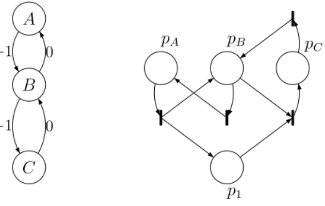
q1 q2

x′

1 = x1+ 1 ∧ x′2 = x2

x′₂ = x2+ 1 ∧ x′1 = x1

Figure 1.3: A Minsky machine

counter values) and an update function (constraints on the way the new counter values are com-puted from the previous ones).

Given a counter system S, a run ρ is a nonempty (possibly infinite) sequence ρ= (q0, ⃗x0), . . . , (qk, ⃗xk), . . .

of configurations such that two consecutive configurations are in the relation −→ from T (S). (q0, ⃗x0) is called the initial configuration of ρ. A run can be alternatively represented by an initial

configuration and a sequence of transitions, assuming that firability holds true for the intermediate configurations and Presburger formulae labelling the transitions define deterministic relations (as in VASS, see Section 1.4.3).

Extensions. Sometimes, we may slightly extend the model of counter systems, for instance by labelling the transitions by a letter from a finite alphabet or by allowing counter values in Z or R. In those cases, we need to interpret the formulae on the adequate structures. Similarly, the transition system can be also defined as a labelled transition system by labelling transition by letters or by transitions. In the sequel, we shall make it clear when we need these slight extensions. In Figure 1.4.1, we present a graphical representation of the counter system corresponding to the Minsky machine made of the two instructions below:

1: C1 := C1+ 1; goto 2

2: C2 := C2+ 1; goto 1

1.4.2 Decision problems

In this section, we enumerate a list of standard decision problems about counter systems. They are mainly related to reachability questions. The list is certainly not exhaustive (model-checking problems can be found in Chapter 2).

(19)

Input: a counter system S and two configurations (q, ⃗x) and (q′_{, ⃗}_x′_).

Question: is there a finite run with initial configuration (q, ⃗x) and final configuration (q′_{, ⃗}_x′_)?

CONTROL STATE REACHABILITY PROBLEM:

Input: a counter system S, a configuration (q, ⃗x) and a control state qf.

Question: is there a finite run with initial configuration (q, ⃗x) and whose final configuration has

control state qf?

CONTROL STATE REPEATED REACHABILITY PROBLEM:

Input: a counter system S, a configuration (q, ⃗x) and a control state qf.

Question: is there an infinite run with initial configuration (q, ⃗x) such that the control state qf is

repeated infinitely often? COVERING PROBLEM:

Input: a counter system S and two configurations (q, ⃗x) and (q′_{, ⃗}_x′_).

Question: is there a finite run with initial configuration (q, ⃗x) and whose final configuration is

(q′_{, ⃗}_x′′_{) with ⃗}_x′ _{≼ ⃗}_x′′_?

BOUNDEDNESS PROBLEM:

Input: a counter system S and a configuration (q, ⃗x).

Question: is the set {(q′_{, ⃗}_x′_{) ∈ Q × N}n_{: (q, ⃗x)}₋_{→ (q}∗ ′_{, ⃗}_x′_{)} finite?}

TERMINATION PROBLEM:

Input: a counter system S and a configuration (q, ⃗x).

Question: is there an infinite run with initial configuration (q, ⃗x)?

Designing algorithms for counter systems can be helpful for instance to verify programs with pointers [BFN04, BBH+06, FLS09], broadcast protocols [EFM99] or systems with energy con-straints [BFL+_{08], see also its use for discrete timed automata (with digital clocks) [DPK03].}

1.4.3 Various classes

In this section, we introduce several subclasses of counter systems by restricting the general defi-nition provided above. Additional requirements can be of distinct nature:

⋆ restriction on syntactic ressources (number of counters, Presburger formulae etc.) ⋆ restriction on the control graph (e.g. flatness),

⋆ semantical restrictions (reversal-boundedness, etc.)

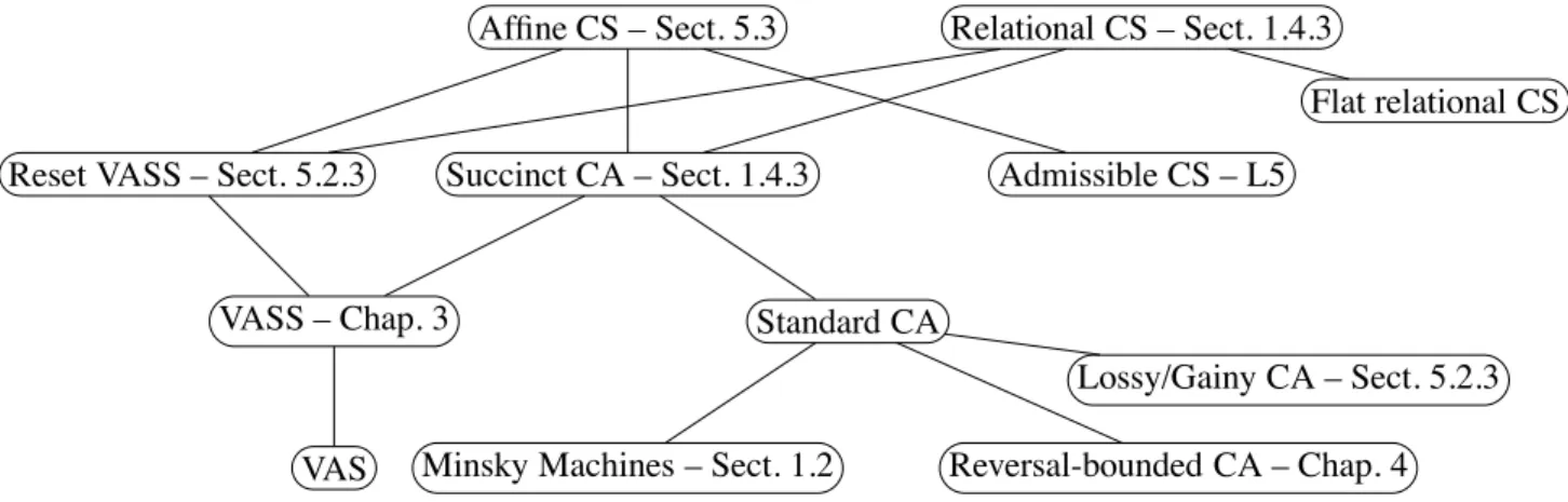
Other subclasses will be considered in this course, but we shall consider them in due course. Our intention in this section is to provide typical examples and results, without being necessarily exhaustive. In Figure 1.4.3, we present (syntactic) inclusions between classes of counter systems (CS stands for ’counter systems’ and CA for ’counter automata’).

(20)

Succinct CA – Sect. 1.4.3

Standard CA VASS – Chap. 3

Reset VASS – Sect. 5.2.3

VAS Minsky Machines – Sect. 1.2 Reversal-bounded CA – Chap. 4 Lossy/Gainy CA – Sect. 5.2.3 Relational CS – Sect. 1.4.3

Affine CS – Sect. 5.3

Flat relational CS Admissible CS – L5

Figure 1.4: Classes of Counter Systems

Relational counter systems

A relational counter system S = (Q, n, δ) is a counter system such that for each transition q −→ϕ q′ ∈ δ, the Presburger formula ϕ is a conjunction of atomic formulae of the form

⋆ either x ∼ y + c, ⋆ or x ∼ c,

where x, y ∈ {x1, . . . , xn, x′1, . . . , x′n}, c ∈ Z and ∼∈ {≥, ≤, =, >, <}. It is worth observing

that other Presburger formulae can define relations between counter values (instead of functions). However, in the sequel, relational counter systems are understood with the above meaning (more general classes are considered in [BIK10]).

Here is an example of formula labelling a transition for n = 2: ϕ = (x1+ 1 < x′1) ∧ (x2− 3 =

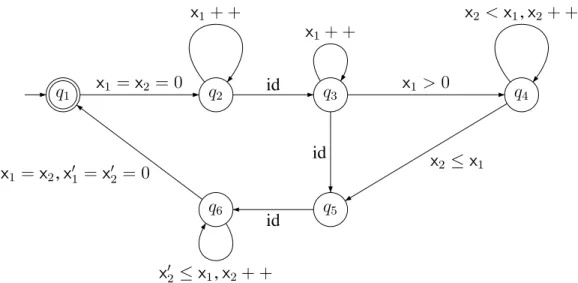
x′₂). The phone controller in Figure 1.1 in which messages are removed can be viewed as a relational counter system (see Figure 1.4.3). In Figure 1.4.3, id preserves the counter values and each variable that does not occur in the expression labelling a transition implicitly preserves its value.

In [CJ98] such systems have been studied and the first result states that the set of Presburger formulae occurring in relational counter systems are closed under composition. For instance, qx ′ 1=x1+1 −−−−→ q′ _{followed by q}′ x′1>x1 −−→ q′′_{is equivalent to} qx ′ 1≥x1+2 −−−−→ q′′ Similarly, q x ′ 1=x′2=x1 −−−−→ q′_{followed by q}′ x′1>x1∧x′2>x2 −−−−−−−→ q′′_{is equivalent to} qx ′ 1>x1∧x′2>x1 −−−−−−−→ q′′

(21)

q1 q2 q3 q4 q6 q5 x1 = x2 = 0 id x1 >0 x2 ≤ x1 id id x₁ = x2, x′1 = x′2 = 0 x₁+ + x1+ + x₂ < x1, x2+ + x′₂ ≤ x1, x2+ +

Figure 1.5: Phone controller (bis)

Lemma 1.4.1. [CJ98] Let S be a relational counter system. Given two transitions t1 = q ϕ1 − → q′ and t2 = q′ ϕ 2 −

→ q′′_{, there exists a Presburger formula ϕ of the form described above for defining}

relational counter systems such that for all ⃗x, ⃗x′_{and ⃗}_x′′_{in N}n_{, we have (q, ⃗x)} t1 −

→ (q′_{, ⃗}_x′₎ t2 −

→ (q′′_{, ⃗}_x′′₎

iff (q, ⃗x)−→ (qt ′′_{, ⃗}_x′′_{) with t = q} ₋_{→ q}ϕ ′′_.

By way of example, the composition of x′

1 ≥ x1+ 1 ∧ x′2 ≤ x2and x1′ ≤ x2∧ x′1 = x′2 leads to

x′₁ ≤ x2∧ x′1 = x′2.

Flat relational counter systems

The key result in [CJ98] states that the transitive closure of transitions occurring in such systems is definable in Presburger arithmetic, see a precise statement in Theorem 1.4.2. The proof is quite difficult; an alternative proof can be found in [BIL09]. For instance, with unique transition t = q x

′ 1=x1+1

−−−−→ q, we have (q, K) −→ (q, K∗ ′_{) iff K}′ _{≥ K. So, the finite iteration of the transition t}

corresponds to the transition q x′1≥x1+1

−−−−→ q. By contrast, with unique transition t = q x′1=x1+2 −−−−→ q, we have (q, K)−→ (q, K∗ ′_{) iff there is k ∈ N such that K}′ _{= K + 2k. Consequently, (q, K)} ₋_{→ (q, K}∗ ′₎

iff valK,K′ |= ∃ y x′₁ = x₁+ 2 × y. Theorem 1.4.2 below generalizes closure under iteration with Presburger arithmetic.

Theorem 1.4.2. [CJ98] Let S be a relational counter system made of a unique transition q −→ q.ϕ One can effectively compute a Presburger formula ϕ′ _{with f ree(ϕ}′_{) = {x}

1, . . . , xn, x′1, . . . , x′n}

such that for all ⃗x, ⃗x′ _{in N}n_{, (q, ⃗x)} ₋_{→ (q, ⃗}∗ _x′_{) iff val} ⃗

x, ⃗x′ |= ϕ′ (where −→ is the transition relation from the transition system T (S)).

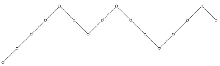
A direct application of the above theorem concerns relational counter systems with restriction on the control graph. A relational counter system is flat whenever, in the control graph, every control state belongs to at most one simple cycle. i.e. with no repeated vertex. Moreover, we

(22)

1.4. CLASSES OF COUNTER SYSTEMS 21 require that there is at most one transition between two control states. Here is an example of flat control graph:

The main result in [CJ98] is the following.

Theorem 1.4.3. [CJ98] Let S be a flat relational counter system and q, q′ _{∈ Q. One can}

effec-tively compute a Presburger formula ϕ such that for all ⃗x, ⃗x′_{in N}n_{, (q, ⃗x)}₋_{→ (q}∗ ′_{, ⃗}_x′_{) iff val} ⃗

x, ⃗x′ |= ϕ (with f ree(ϕ) = {x1, . . . , xn, x′₁, . . . , x′n}).

The proof goes roughly as follows. Lemma 1.4.1 allows to compute the effects of each simple cycle and by flatness the number of simple cycles is bounded by card(Q). Then, Theorem 1.4.2 allows to compute the effects of passing a finite number of times on each simple cycle. Flatness guarantees that reaching a control state from another control state implies passing through the simple cycles in a regular manner which can be mimicked at the level of formulae.

Consequently,

Corollary 1.4.4. The reachability problem for flat relational counter systems is decidable. The corollary can be obtained as follows. Consider the instance S, (q, ⃗y) and (q′, ⃗y′_{). We have}

seen that we can compute the Presburger formula ϕ that encodes the reachability relation in S. It remains to check satisfiability of the formula below:

(

i=n

'

i=1

(xi = ⃗y(i) ∧ x′i = ⃗y′(i))) ∧ ϕ

assuming free variables in ϕ are x1, . . . , xn, x′1, . . . , x′n. This can be done since the satisfiability

problem for Presburger arithmetic is decidable. Other types of counter systems with semilinear reachability sets can be found in [Iba78, HP79, Esp97, FS00, FL02, Ler03, LS05, FS08]. A generalization has been also considered in [BIK10].

(23)

Succinct counter automata

In the sequel, we adopt the convention that a counter automaton is a counter system in which the instructions are either zero-tests, increments or decrements, possibly encoded succinctly. A

succinct counter automaton is a counter system (Q, n, δ) in which the transitions are of the form

either qinc(⃗b)−−→ q′ _{with ⃗b ∈ Z}n_{or q} _{−−−→ q}zero(⃗b′) ′ _{with ⃗}_b′ _{∈ {0, 1}}n_where

⋆ inc(⃗b) is a shortcut for(_i∈[1,n]x′_i = xi+ ⃗b(i),

⋆ zero(⃗b′_{) is a shortcut for} (

i∈[1,n] s.t. ⃗b′_(i)=1xi = 0 ∧

(

i∈[1,n]x′i = xi (as usual, empty

con-junction is understood as ⊤).

In succinct counter automaton, each transition either performs zero-tests on a subset of counters or updates counters by adding a vector in Zn_{. All the counters are tested or updated simulateously.}

It is easy to check that every succinct counter automaton is a relational counter system.

Standard counter automata

A standard counter automaton is a counter system (Q, n, δ) in which the transitions are of the form either q inc(i)−−→ q′ _{or q} dec(i)_{−−→ q}′ _{or q}zero(i)_{−−−→ q}′ _{(i ∈ [1, n]) where}

⋆ inc(i) is a shortcut for (x′

i = xi+ 1) ∧ (

(

j̸=ix′j = xj) (also written xi++),

⋆ dec(i) is a shortcut for (x′

i = xi− 1) ∧ ((_j̸=ix′j = xj) (also written xi- -),

⋆ zero(i) is a shortcut for (xi = 0) ∧ ((_jx′j = xj) (also written xi = 0?).

By contrast to succinct counter automata, transitions in standard counter automata can perform a simple operation at once (otherwise, a succession of transitions is needed). Indeed, standard counter automata and succinct counter automata are very similar but when it comes to complexity issues, exponential blow-up may occur when passing from one model to another. In the sequel, unless otherwise stated, by a counter automaton we mean a standard one.

It is easy to check that Minsky machines (with two counters) form a subclass of standard counter automata.

Vector addition systems with states

A vector addition system with states [KM69] (VASS for short) is a succinct counter automata without zero-tests, i.e. all the transitions are of the form q inc(⃗b)−−→ q′ _{with ⃗b ∈ Z}n_{. In the sequel, a}

VASS is represented by a tuple V = (Q, n, δ) where Q is the finite set of control states and δ is a finite subset of Q × Zn_{× Q.}

Standard counter automata can be naturally viewed as vector addition systems with states aug-mented with zero-tests by simulating transitions of the form q −→ q⃗b ′ _{by sequences of increments}

and decrements.

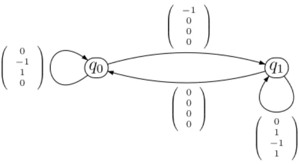
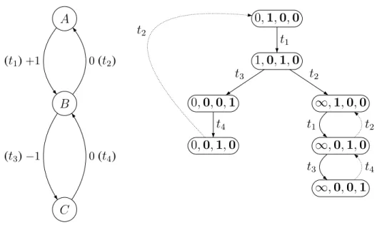
Figure 1.6 presents an example of VASS. As an exercise, one can show that for all ⃗x ∈ N4_{, the}

set {⃗y ∈ N4 _{: (q} 0, ⃗x)

∗

−

(24)

1.4. CLASSES OF COUNTER SYSTEMS 23 q0 q1 0 B B @ −1 0 0 0 1 C C A 0 B B @ 0 0 0 0 1 C C A 0 B B @ 0 1 −1 1 1 C C A 0 B B @ 0 −1 1 0 1 C C A

Figure 1.6: A VASS weakly computing multiplication

A vector addition systems (VAS for short) is defined as a VASS with a unique control state. In the sequel, a VAS T is represented by a finite subset of Zn _{corresponding to its set of transitions.}

VASS and VAS are be viewed as equivalent models, see e.g. [Reu90]. Moreover, for many prob-lems such as covering or boundedness, the probprob-lems on VASS and Petri nets are equivalent (see Chapter 3).

Theorem 1.4.5. [May84, Kos82, Reu90, Lam92] The reachability problem for VASS is decid-able.

This famous result has been the subject of the book [Reu90] since the proof requires many steps involving expertise in graph theory, logic, theory of well-quasi orderings etc. Nevertheless, the exact complexity of the reachability problem is open: we know it is EXPSPACE-hard [Lip76, CLM76, Esp98] and no primitive recursive upper bound exists. By contrast, the covering problem and boundedness problems seem easier.

Theorem 1.4.6. [Lip76, Rac78] The covering and boundedness problems for VASS are EX -PSPACE-complete.

Decidability is established in [KM69] but with a worst-case non primitive recursive bound (see Section 3.3). The EXPSPACE lower bound is due to Lipton and the upper bound to Rackoff

(see Section 3.4). In order to be precise, one should explain how vectors in Zn_{are encoded. The}

upper bound holds true with a binary representation of integers whereas the lower bound holds true already with the values -1, 0 and 1. Consequently, the problem is EXPSPACE-hard even with

an unary encoding. In general, the less the encoding is concise, the more difficult hardness results are possible. We shall present the proof for the upper bound in Chapter 3. Observe also that the covering problem can also express the thread-state reachability problem for replicated finite-state programs, see e.g. [KKW10] as well as decision problems for the parameterized verification of ad-hoc networks [DSZ10]. Similarly, the boundedness problem for asynchronous programs has been considered in [GaAR09].

The operation of resetting a counter consists in providing the value zero to the counter. For instance reset(i) can be defined as the formula (x′

i = 0) ∧ (

(

j̸=ix′j = xj) A reset VASS is defined

as a VASS except that we allow transitions labelled by reset(i). It is worth noting that the bound-edness and the reachability problems for reset VASS become undecidable, see e.g. [DFS98]. By contrast, the covering problem for reset VASS is decidable by using the theory of well-structured transition systems, see e.g. [FS01].

(25)

1.5 Exercises

Exercise 1.5.1. Let ϕ be a Presburger formula with more than one free variable. Define a

Pres-burger formula ψ such that ψ is satisfiable iff REL(ϕ) is finite.

Exercise 1.5.2. Let X ⊆ N2 _{be a semilinear set. Show that {k ∈ N : (k, k}′_{) ∈ X} (projection) is}

a semilinear subset of N.

Exercise 1.5.3. Define a Presburger formula ϕ such that REL(ϕ) = {(n1, n2) ∈ N × N : n1 ×

n2 is odd}.

Exercise 1.5.4. Show that any arithmetic progression (viewed as a set of natural numbers) can be

defined in Presburger arithmetic.

Exercise 1.5.5. Show that a set X of natural numbers is semilinear iff there are N, M ∈ N such

that for every n ≥ N, n ∈ X iff n + M ∈ X (X is ultimately periodic). Conclude that the sets {2i _{: i ∈ N} and {i}2 _{: i ∈ N} are not semilinear.}

Exercise 1.5.6. Show that semilinear sets are Presburger definable.

Exercise 1.5.7. Let X, Y ⊆ Nn_{. We define X + Y as the set {⃗x + ⃗y : ⃗x ∈ X, ⃗y ∈ Y }. Show that}

if X and Y are semilinear, then X + Y is also semilinear.

Exercise 1.5.8. Dickson’s Lemma [Dic13] states that for any ω-sequence ⃗x0, ⃗x1, . . .of tuples in

Nn_{, there are i < j such that ⃗}_x_i _{≼ ⃗}_x_j_{. Show Dickson’s Lemma.}

Exercise 1.5.9. Let S = (Q, n, δ) be a VASS and (q0, ⃗x0) be a configuration. Using Dickson’s

Lemma, show the equivalence between the two statements below: ⋆ There is an infinite run with initial configuration (q0, ⃗x0).

⋆ There exist a finite run (q0, ⃗x0), . . . , (qk, ⃗xk) and k′ < ksuch that qk′ = q_kand ⃗x_k′ ≼ ⃗x_k. Does the equivalence hold true for VASS with resets? for standard counter automaton?

Exercise 1.5.10. Let us consider the VASS S presented in Figure 1.6. Determine the set of initial

configurations such that S is terminating from them.

Exercise 1.5.11. Consider the counter system obtained from Figure 1.1 by deleting the

communi-cation labels (of the form either a! or b?). Show that the set {⃗x ∈ N2 _{: (q} 1,⃗0)

∗

−

→ (qi, ⃗x), i ∈ [1, 6]}

is semilinear.

Exercise 1.5.12. Check the statement in Lemma 1.4.1 with

ϕ1 = x′1 ≥ x1+ 1 ∧ x2′ ≤ x2 ϕ2 = x′1 ≤ x2∧ x′1 = x′2 ϕ= x1′ ≤ x2∧ x′1 = x′2

Exercise 1.5.13. Show the following equality for the VASS defined in Figure 1.6:

{) ab d * ∈ N3 _{: d ≤ a × b} =} {) ab d * ∈ N3 : ∃) a ′ b′ c′ * ∈ N3, run (q0, # a b 0 0 $ )−→ (q∗ 0, # a′ b′ c′ d $ )}

(26)

Chapter 2 Linear-Time Temporal Logics

This chapter is mainly dedicated to present a linear-time temporal logic LTLCS(PrA) whose mod-els are infinite runs from counter systems. First, we recall the definitions for standard linear-time temporal logic LTL as well as its automata-based approach with B¨uchi automata. Then, we define the very expressive logic LTLCS(PrA) and its two fragments CLTL(PrA) (Presburger LTL) and LTL with registers (LTL↓_{) obtained by restricting the first-order quantification over counter values.}

The chapter concludes by providing the decidability status for several fragments for CLTL(PrA) and LTL↓_{. In the subsequent chapters, we shall refer to these logics to state the decidability status}

of satisfiability and model-checking problems.

2.1 Temporal Modalities on Computations

Temporal logics contain modalities with a temporal interpretation. A modality is usually defined as a syntactic object (term) that modifies the relationships between a predicate and a subject. For example, in the sentence “Tomorrow, it will rain”, the term “Tomorrow” is a temporal modality. Temporal logics make use of different types of modalities and we recall below some of them interpreted over runs (a.k.a. executions or ω-sequences). The temporal modalities (also known as temporal operators) allow one to speak about the sequencing of states along an execution, rather than about the states taken individually. The simplest temporal operators are X (“neXt”), F (“sometimes”) and G (“always”). Below, we shall freely use the Boolean operators ¬ (negation), ∨ (disjunction), ∧ (conjunction) and ⇒ (material implication).

⋆ Whereas ϕ states a property of the current state, Xϕ states that the next state (X for “neXt”) satisfies ϕ. For example, ϕ ∨ Xϕ states that ϕ is satisfied now or in the next state.

Xp p

Xp: next-time p

⋆ Fp announces that a future state (F for “Future”) satisfies ϕ without specifying which state, and Gϕ that all the future states satisfy ϕ. These two operators can be read informally as “ϕ will hold some day” and “ϕ will always be”.

(27)

Fp p Fp: sometimes p

Duality The operator G is the dual of F: whatever the formula ϕ may be, if ϕ is always

satisfied, then it is not true that ¬ϕ will some day be satisfied, and conversely. Hence Gϕ and ¬F¬ϕ are equivalent.

Gp, p p p p p

Gp: always p

By way of example, the expression alert ⇒ F halt means that if we (currently) are in a state of alert, then we will (later) be in a halt state.

⋆ The temporal operator U (for “Until”) is richer and more complicated than the temporal operator F. ϕ1Uϕ2 states that ϕ1 is true until ϕ2 is true. More precisely: ϕ2 will be true

some day, and ϕ1will hold in the meantime.

pUq, p p p p q

pUq: p until q

The example G(alert ⇒ F halt) can be refined with the statement that “starting from a state of alert, the alarm remains activated until the halt state is eventually reached”:

G(alert ⇒ (alarm U halt)).

Sometime operator. The temporal operator F is a special case of U: Fϕ and true U ϕ are equivalent.

Weak until. There exists also a “weak until”, denoted W. The statement ϕ1Wϕ2 still

ex-presses “ϕ1Uϕ2”, but without the inevitable occurrence of ϕ2 and if ϕ2 never occurs, then

ϕ1 remains true forever. So, ϕ1Wϕ2 is equivalent to Gϕ1∨ (ϕ1Uϕ2).

2.2 Linear-Time Temporal Logic LTL

As far as we know, linear-time temporal logic LTL in the form presented herein has been first considered in [GPSS80] based on the early works [Kam68, Pnu77]. The version of LTL with explicitely the time and until operators first appeared in [GPSS80]. Surprisingly, the next-time operator has been introduced in [MP79] in order to define LTL restricted to the next-next-time and sometime operators (see also a similar language in [Pnu79]). Nowadays, LTL is one of the most used logical formalisms to specify the behaviours of computer systems in view of formal

(28)

2.3. A BRIEF INTRODUCTION TO B ¨UCHI AUTOMATA 27 verification. It has been also the basis for numerous specification languages such as PSL [EF06]. Moreover, it is used as a specification language in tools such as SPIN [Hol97] and SVM [McM93]. Let us provide below a few definitions about LTL. LTL formulae are built from the following abstract grammar:

ϕ, ψ ::= p | ¬ϕ | ϕ ∧ ψ | ϕ ∨ ψ | Xϕ | ϕUψ where p ranges over a countably infinite set PROP of propositional variables.

⇔ there is j ≥ i such that ρ, j |= ϕ2 and ρ, k |= ϕ1for all i ≤ k < j.

As usual, we pose Fϕ = ⊤Uϕ and Gϕdef = ¬F¬ϕ. Observe that ψdef 1Uψ2 is equivalent to ψ2∨ (ψ1 ∧

Xψ1Uψ2).

Given a LTL formula ϕ, we write Models(ϕ) to denote the set of sequences ρ in P(PROP)ω

such that ρ, 0 |= ϕ. We recall below that Models(ϕ) can be effectively represented by a B¨uchi au-tomaton Aϕ(see basics in Section 2.3), namely Aϕrecognizes exactly the sequences in Models(ϕ).

2.3 A Brief Introduction to B ¨uchi Automata

Automata-based approach

The automata-based approach consists in reducing logical problems into automata-based decision problems in order to take advantage of known results from automata theory. Alternatively, this can be viewed as a means to transform declarative statements (typically formulae) into opera-tional devices (typically automata with sometimes rudimentary computaopera-tional power). The most standard target problems on automata used in this approach are the following:

⋆ the nonemptiness problem checks whether an automaton admits at least one accepting com-putation (in symbols L(A) ̸= ∅?),

⋆ the universality problem checks whether an automaton accepts everything (of course this needs to be made more precise depending on the objects we are dealing with, words, trees etc.),

⋆ the inclusion problem checks whether the language accepted by the automaton A is in-cluded in the language accepted by the automaton B (in symbols L(A) ⊆ L(B)?).

(29)

A =

a b

b a

Figure 2.1: L(A) = {σ ∈ {a, b}ω _{| |σ|}

a = ω}

A pioneering work is due to Büchi [Büc62] in which Büchi automata are shown equivalent to formulae in monadic second-order logics (MSO) over (N, <); models of a formula built over the second-order variables P1, . . . , PN are ω-sequences over the alphabet P({P1, . . . , PN}). In full

generality, here are a few desirable properties of the approach.

⋆ The reduction should be conceptually simple, apart from being semantically faithful.

⋆ The computational complexity of the automata-based target problem should be well-characterized. In that way, one gets a complexity upper bound for solving the source logical problem.

⋆ Last but not least, preferrably, the reduction should allow obtaining the optimal complexity for the source logical problem.

In this chapter, we shall present the automata-based approach for solving logical problems in-volving temporal logics (see also Chapter 5). However, nowadays this approach is quite active and among the trends one can distinguish the development of algorithmic automata theory (for instance to design efficient decision procedures for testing nonemptiness, complementing etc., see e.g. [GS09]) and the appearance of new source problems (see e.g. axiom pinpointing in [BP08]).

B ¨uchi automata in a nutshell

A B¨uchi automaton is defined as a finite-state automaton that accepts ω-words instead of finite words. Formally, a B¨uchi automaton A is a tuple A = (Σ, Q, Q0, δ, F) such that

⋆ Σ is a finite alphabet, ⋆ Qis a finite set of states,

⋆ Q0 ⊆ Q is the set of initial states,

⋆ the transition relation δ is a subset of Q × Σ × Q, ⋆ F ⊆ Q is a set of final states.

Given q ∈ Q and a ∈ Σ, we also write δ(q, a) to denote the set of states q′ _{such that (q, a, q}′_{) ∈ δ.}

A run ρ of A is a sequence q0 a0 − → q1 a1 −

→ q2. . . such that q0 ∈ Q0 and for every i ≥ 0,

(qi, ai, qi+1) ∈ δ (also written qi ai −

→ qi+1). The run ρ is successful if some state of F is repeated

infinitely often in ρ: inf(ρ) ∩ F ̸= ∅ where we let inf(ρ) = {q ∈ Q : ∀ i, ∃ j > i, q = qj}. The

label of ρ is the word σ = a0a1· · · ∈ Σω. The automaton A accepts the language L(A) made of

ω-words σ ∈ Σω_{such that there exists a successful run of A on the word σ, i.e., with label σ. For}

instance, the automaton in Figure 2.1 accepts those words over {a, b} having infinitely many a’s (the initial states are marked with an incoming arrow and the states in F are doubly circled).

(30)

2.3. A BRIEF INTRODUCTION TO B ÜCHI AUTOMATA 29 Now, we introduce a standard generalization of the Büchi acceptance condition by considering conjunctions of classical Büchi conditions. A generalized Büchi automaton (GBA) is a structure

A = (Σ, Q, Q0, δ,{F1, . . . , Fk})

such that F1, . . . , Fk⊆ Q and Σ, Q, Q0and δ are defined as for B¨uchi automata. A run is defined

as for B¨uchi automata and a run ρ of A is successful iff for 1 ≤ i ≤ n, we have inf(ρ) ∩ Fi ̸=

∅. Lemma 2.3.1 below simply states each GBA A can be easily translated into a classical BA, preserving the language of accepted ω-words.

Lemma 2.3.1. Let A = (Σ, Q, Q0, δ,{F1, . . . , Fk}) be a generalized B¨uchi automaton. One can

compute, in logarithmic space in the size of A, a B¨uchi automaton Ab _{= (Σ, Q}b_{, Q}b

0, δb, Fb) such

that L(Ab_{) = L(A).}

Proof: Let A = (Σ, Q, Q0, δ,{F1, . . . , Fk}) be a generalized B¨uchi automaton. The idea of

the proof consists in defining Ab _{from k copies of A and to simulate the generalized accepting}

condition by passing from one copy to another. 1. Qb def = Q × {1, . . . k}, 2. Qb 0 def = Q0× {1}, 3. Fb def = F1× {1},

4. δb_{((q, i), a) is defined as the union of the two following sets}

(a) {(q′_{, i) : q}₋_{→ q}a ′ _{∈ δ, q ̸∈ F}

i} (stay in the same copy if no final state in Fiis reached),

(b) {(q′_,_{(i mod k) + 1) : q} ₋_{→ q}a ′ _{∈ δ, q ∈ F}

i} (go to the next copy if a final state in Fi is

reached).

One can check that A and Ab_{accept the same language. QED}

The class of languages accepted by B¨uchi automata admits various characterizations, for in-stance it corresponds to the class of ω-regular languages. On the logical side, such languages correspond exactly to the set of models satisfied by formulae from LTL augmented with automata-based temporal operators [Wol83]. There exist alternative characterizations, see e.g. [Var88]. Proposition 2.3.2. The family of ω-regular languages is closed by intersection, union and com-plementation.

The proof for union is similar to the proof for standard finite-state automata, the proof for intersection uses an idea similar to the proof of Lemma 2.3.1. By contrast, the closure by comple-mentation is much more difficult to show, see e.g. [B¨uc62, Tho99, Muk09] (see also [FKV04]).

The nonemptiness problem for B¨uchi automata is defined as follows:

Input: a B¨uchi automaton A, Question: is L(A) ̸= ∅?

(31)

{p′_{}, {p, p}′_}

{p}, {p, p′_}

Σ

Figure 2.2: An automaton for pUp′_models

In order to characterize the computational complexity of the nonemptiness problem, we can use the lemma below.

Lemma 2.3.3. Let A = (Σ, Q, Q0, δ, F) be a B¨uchi automaton. L(A) ̸= ∅ iff there is a path in

the graph (Q, {(q, q′_{) : ∃a s.t. q} ₋_{→ q}a ′ _{∈ δ}) of the form q} 0

∗

−

→ q−→ q with q+ 0 ∈ Q0 and q ∈ F .

Proposition 2.3.4. [VW94] The nonemptiness problem for B¨uchi automata is NLOGSPACE

-complete.

By contrast, the universality problem for B¨uchi automata is PSPACE-complete, see e.g., [SVW87].

2.4 From Formulae to Automata

Here we will show that given an LTL formula ϕ built over the set of propositional variables {p1, . . . ,pN}, it is possible to effectively construct a B¨uchi automaton Aϕ over the alphabet

{p1, . . . ,pN} such that L(Aϕ) = Models(ϕ).

Figure 2.2 presents a B¨uchi automaton A such that L(A) = Models(pUp′_{) with Σ = {p, p}′_}.

We wish to define Aϕ from ϕ in a systematic and optimal way. This allows us to obtain optimal

complexity bounds and if the construction of automata is optimized, it can also provide efficient algorithms.

Proposition 2.4.1. [VW94] For every LTL formula ϕ, there is a B¨uchi automaton Aϕ such that

1. L(Aϕ) = Models(ϕ),

2. |Aϕ| is in 2O(|ϕ|)and,

(32)

2.4. FROM FORMULAE TO AUTOMATA 31 In Proposition 2.4.1, it should be understood that the set of propositional variables PROP is restricted to the atomic formulae occurring in ϕ. Below, we explain how Aϕ is defined from ϕ

without providing the formal proofs.

Definition 2.4.1. Let ϕ be an LTL formula. The closure of ϕ, denoted by cl(ϕ) is the smallest set

⋆ containing the subformulae of ϕ,

⋆ closed under negation (we identify ¬¬ψ with ψ), ⋆ if χ1Uχ2 ∈ cl(ϕ), then X(χ1Uχ2) ∈ cl(ϕ).

∇ The closure set contains all the formulae we need to consider to check satisfiability and the cardinality of cl(ϕ) is linear in the size of ϕ. An atom X is a subset of cl(ϕ) satisfying the conditions below:

1. for all formulae ψ in cl(ϕ), ψ ∈ X iff ¬ψ ̸∈ X, 2. ψ1∧ ψ2 ∈ X iff ψ1, ψ2 ∈ X,

3. ψ1∨ ψ2 ∈ X iff ψ1 ∈ X or ψ2 ∈ X.

An atom is nothing but a maximally consistent subset of cl(ϕ). A pair of atoms (X, X′) is said to be one-step consistent iff the conditions below hold true:

⋆ if ψ1Uψ2 ∈ X, then ψ2 ∈ X or (ψ1 ∈ X and ψ1Uψ2 ∈ X′),

⋆ for Xψ ∈ cl(ϕ), Xψ ∈ X iff ψ ∈ X′_.

Now, let us define Aϕbased on the previous definitions. Aϕis actually a generalized B¨uchi

au-tomaton that can be converted into a standard B¨uchi auau-tomaton. So Aϕ = (Σ, Q, Q0, δ, F1, . . . , Fα)

with:

⋆ Σ = P({p1, . . . ,pN}) (set of propositional variables occurring in ϕ),

⋆ Qis the set of atoms (its cardinality is exponential in the size of ϕ), ⋆ Q0is the subset of atoms containing ϕ,

⋆ X −→ Y ∈ δ iff a = {pa 1, . . . ,pN} ∩ X and (X, Y ) is one-step consistent,

⋆ for each until formula ψ1Uψ2, there is exactly one set Fi such that Fi = {X ∈ Q :

either ψ1Uψ2 ̸∈ X or ψ2 ∈ X}.

Each control state X ∈ Q is a set of formulae that are intended to be satisfied at the current position. Either this satisfaction can be checked locally (typically for Boolean formulae using the fact that X is an atom) or the transition relation of Aϕallows us to propagate the constraints.

Accepting conditions F1, . . . , Fα (indexed by until formulae occurring in ϕ) guarantee that the

search for witnesses is not delayed forever. In particular, they forbid postponing forever the satisfaction of ψ2when ψ1Uψ2has to be satisfied.

(33)

Proposition 2.4.2. L(Aϕ) = Models(ϕ).

The equality is obtained by establishing the two following properties.

⋆ Given a model ρ : N → P({p1, . . . ,pN}) ∈ Models(ϕ), i.e. ρ, 0 |= ϕ, there is a unique

accepting run X0 ρ(0) −→ X1 ρ(1) −→ X2 ρ(2)

−→ · · · in Aϕ such that for all i ≥ 0 and ψ ∈ cl(ϕ), we

have ψ ∈ Xi iff ρ, i |= ψ.

⋆ Conversely, for each accepting run X0 a0 − → X1 a1 − → X2 a2 −

→ · · · in Aϕ, the model ρ defined by

ρ(i) = ai for i ≥ 0 satisfies that for i ≥ 0 and ψ ∈ cl(ϕ), we have ψ ∈ Xiiff ρ, i |= ψ.

In the sequel, we write Aϕto denote the B¨uchi automaton recognizing Models(ϕ).

2.5 Full Presburger LTL for Counter Systems

Linear-time temporal logic LTL equipped with “next-time” operator X, “until” operator U and their past-time counterparts is known to be equivalent to first-order theory of order [Kam68]. Satisfi-ability and model-checking problems for LTL (even with past-time operators) are known to be PSPACE-complete [SC85]. In spite of these nice features, it is worth recalling that a propositional variable p only represents a property of the current configuration of the system. For instance, p may hold true whenever the value of the variable x is greater than the value of the variable y after running the current instruction. A more satisfying solution is to include in the logical language the possibility to express directly constraints between variables of the program, whence giving up the standard abstraction made with propositional variables. When the variables are typed, they may be interpreted in some specific domain like integers, real numbers, strings and so on; reasoning in such theories can be performed thanks to satisfiability modulo theories proof tech-niques, see e.g., [BSST08] and [GNRZ07] in which SMT solvers are used for model-checking infinite-state systems. Hence, a proposition like “x is greater than the next value of y” can be encoded in such extended temporal logics by x > Xy but this time the models are sequences of configurations. This means that each position comes with a control state and a valuation for variables. Hence, the basic idea behind the design of the logic LTLCS(PrA) is to refine the lan-guage of atomic formulae and to allow the possibility to compare counter values at successive positions of the run of the counter systems. Similar motivations can be found in the introduc-tion of concrete domains in descripintroduc-tion logics, that are logic-based formalisms for knowledge representation [BH91, Lut03, Lut04].

We define below a version of linear-time temporal logic LTL dedicated to counter systems in which the atomic formulae are Presburger formulae about counter values, the temporal operators are those of LTL and first-order quantification over natural numbers is allowed, although we shall use it in a restricted way. The main advantage of defining a so general language is that it is then easy to compare the different languages in a uniform framework. Similarly, in [MP95], a mixture of first-order logic and LTL is shown sufficient to precisely state verification problems for the class of reactive systems.

We introduce a countable set of integer variables, say VARp = {y1, y2, . . .}, for quantification

over natural numbers. Elements of VARp are distinct from the counter variables in VAR = {x1, x2, . . .} that are free variables, only interpreted by the counter values on configurations. We