Multiscale simulations of the early stages of the growth of graphene on copper

(1)

RESEARCH OUTPUTS / RÉSULTATS DE RECHERCHE

Author(s) - Auteur(s) :

Publication date - Date de publication :

Permanent link - Permalien :

Rights / License - Licence de droit d’auteur :

Bibliothèque Universitaire Moretus Plantin

Institutional Repository - Research Portal

Dépôt Institutionnel - Portail de la Recherche

researchportal.unamur.be

University of Namur

Multiscale simulations of the early stages of the growth of graphene on copper

Gaillard, P.; Chanier, T.; Henrard, L.; Moskovkin, P.; Lucas, S.

Published in:

Surface Science

DOI:

10.1016/j.susc.2015.02.014

Publication date:

2015

Link to publication

Citation for pulished version (HARVARD):

Gaillard, P, Chanier, T, Henrard, L, Moskovkin, P & Lucas, S 2015, 'Multiscale simulations of the early stages of

the growth of graphene on copper', Surface Science, vol. 637-638, 20440, pp. 11-18.

https://doi.org/10.1016/j.susc.2015.02.014

General rights

Copyright and moral rights for the publications made accessible in the public portal are retained by the authors and/or other copyright owners and it is a condition of accessing publications that users recognise and abide by the legal requirements associated with these rights. • Users may download and print one copy of any publication from the public portal for the purpose of private study or research. • You may not further distribute the material or use it for any profit-making activity or commercial gain

• You may freely distribute the URL identifying the publication in the public portal ?

Take down policy

If you believe that this document breaches copyright please contact us providing details, and we will remove access to the work immediately and investigate your claim.

(2)

Multiscale simulations of the early stages of the growth of graphene

on copper

P. Gaillard

⁎

, T. Chanier

1

, L. Henrard, P. Moskovkin, S. Lucas

Research center in physics of matter and radiation (PMR), University of Namur, 61 rue de Bruxelles, 5000 Namur, Belgium Research group on carbon nanostructures (CARBONAGe), University of Namur, 61 rue de Bruxelles, 5000 Namur, Belgium

a b s t r a c t

a r t i c l e i n f o

Article history:

Received 19 December 2014 Accepted 24 February 2015 Available online 5 March 2015 Keywords:

Growth Graphene Simulations Ab initio Kinetic Monte Carlo

We have performed multiscale simulations of the growth of graphene on defect-free copper (111) in order to model the nucleation and growth of grapheneflakes during chemical vapour deposition and potentially guide future experimental work. Basic activation energies for atomic surface diffusion were determined by ab initio calculations. Larger scale growth was obtained within a kinetic Monte Carlo approach (KMC) with parameters based on the ab initio results. The KMC approach counts thefirst and second neighbours to determine the probability of surface diffusion. We report qualitative results on the size and shape of the graphene islands as a function of depositionflux. The dominance of graphene zigzag edges for low deposition flux, also observed experimentally, is explained by its larger dynamical stability that the present model fully reproduced.

1. Introduction

Graphene is a material that has recently attracted considerable attention due to its exceptional mechanical, electrical or optical properties[1–3]and its status as a model 2D system. Grapheneflake synthesis can be achieved by multiple methods such as mechanical exfoliation[4]and chemical vapour deposition (CVD). In this article we consider the synthesis of graphene through CVD on copper (111) substrates, though CVD can be achieved on many other substrates such as Ni or Pt[5]. CVD on copper substrates is advantageous as it can produce large area thin (monolayer)flakes of graphene[6](this can also be achieved on other substrates[7,8]). However, implementa-tion of graphene devices requires effective control of the quality of the film. Understanding the growth mechanisms is therefore important for the improvement of the quality of the grown layer. For example, a large amount of nucleation tends to create grain boundaries that can deteriorate the electrical conductivity[9]. This problem has been exten-sively studied experimentally[10,11], but no complete atomic model of the growth has yet been proposed (see below).

CVD of graphene on copper is a relatively high temperature process (usually 1273 K, with copper melting at 1357 K) that uses a combination of gases (i.e., methane and hydrogen) in a chamber[6,12]. At an atomic level, CVD growth of graphene on Cu is initiated with the adsorption and dissociation of methane on the surface. The C adatoms then diffuse on

the surface and form small nuclei that, eventually, grow into larger islands[13]. Experimental articles have pointed out the inﬂuence of hydrogen partial pressure[14], chamber pressure[15], state and orien-tation of the substrate[16]and temperature[17]on the size and shape of graphene domains. Many different shapes have been observed, such as hexagons[9,18,19], multiple-lobed islands[20,21], snowﬂake-like graphene[13]or hexagons with dendritic edges[20].

Various approaches have been reported to model or simulate the growth of graphene. For the specific case of CVD growth, at the macro-scopic level, thermodynamic calculations of gas phase equilibrium in the CVD chamber[22]have been proposed to correlate to gas phase species with the graphenefilm growth. The decomposition of hydrocar-bon on copper and the growth of small islands has been studied by first-principle thermodynamics [23]. Models of nucleation and growth during CVD (including qualitative models, such as[11]), explained the role of hydrogen[24]and can include calculations of the density of nuclei[17]. Monte Carlo studies have covered the evolution of defects [25], or growth mechanisms of graphene[26]. At the atomic level, stabil-ity and diffusion of carbon atoms and dimers have been evaluated by DFT ab-initio calculations for perfect[27]and stepped[28]copper surfaces. Surface adsorption has been found to be favourable on a Cu (111) surface for isolated atoms but surface orientation is less important for small clusters of carbon atoms[29]. Ab-initio methods have also demonstrated the stability of zig-zag edges based on static calculations for small carbon clusters on a perfect Cu (111) surface[18]or related to the presence of“free” Cu atoms on the surface[30].

Beside these macroscopic or ab-initio calculations, Kinetic Monte Carlo (KMC) simulations provide a large-scale atomistic view with an insight into the dynamics of the growth process going from atomic

⁎ Corresponding author.

E-mail address:philippe.gaillard@unamur.be(P. Gaillard).

1

Now at Laboratoire de Spectrométrie et Optique Laser, EA 938, Université de Brest, 6 avenue Victor Le Gorgeu, F-29285 Brest Cedex, France.

http://dx.doi.org/10.1016/j.susc.2015.02.014

Contents lists available atScienceDirect

Surface Science

(3)

diffusion to cluster formation. KMC has been used to model the growth of numerous nanomaterials[31–33]but, to the best of our knowledge, not for graphene. Exceptions are pattern formation during growth, based on the a priori presence of carbon island and on the attachment of small clusters[13]and the study of vacancy migration[34].

In this article, we focus on the speci_{fic case of the simulations of the} early stages of the growth of graphene on Cu (111) by CVD. Wefirst present ab initio calculations for the surface diffusion activation energies for a few typical cases. Secondly, we present our KMC modelling scheme and compare results obtained when atomic diffusion depends onfirst neighbours only and when it also depends on second neighbours. Our KMC algorithm takes into account the effect of detachment from carbon clusters and atomic diffusion, and does not require seeds or steps to obtain grapheneflakes. Our project is therefore to implement multiscale simulations with thefirst scale being ab initio and the second scale the KMC simulations. Our main results are on the qualitative effect of the deposition rates on the graphene island shape that can be compared to experimental results. We also note that, at low depositionflux, our flake edges are mainly zigzag, with armchair edges being relatively rare. This result is in agreement with experimental data and other models[14,18,35].

2.Ab initio calculations

Plane wave supercell calculations were carried out to determine activation energies of diffusion events of carbon atoms on Cu (111) sub-strate by using the VASP5.3 code[36,37]with the projector augmented wave method[38](PAW). We applied the standard C and Cu PAW-potentials[38]from the VASP5.2 database. Cu 3d electrons were treated as valence electrons. The valence wave functions were expanded by plane waves with a kinetic energy cut-off Ecut= 420 eV. We used the

generalized gradient approximation (GGA) in the parametrization of Perdew–Burke–Ernzerhof[39]. We considered graphene on top of a free Cu (111) surface. The substrate consists of a 9 monolayer thick Cu (111) substrate (seeFig. 1). We used the Cu bulk equilibrium GGA lattice constant of 3.63 Å. Free Cu (111) substrate coordinates were fully relaxed and thenﬁxed throughout the study.

A previous GGA study determined that fcc and hcp positions were the most stable sites for single carbon adsorption even if between sites might play a role[27]. More recently, it was demonstrated that for small graphene islands on Cu (111) carbon atoms preferentially adsorbed on fcc and hcp sites[40]. We then considered these adsorption sites in the present study.

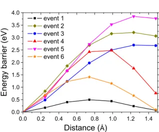
We have estimated the diffusion barrier by moving one carbon atom linearly from one conﬁguration to the other. We have considered 5 equidistant images for each calculation. The carbon in-plane coordi-nates were keptﬁxed with only the z coordinates allowed to relax. The list of diffusion events that were considered (where the numbers correspond to the event number inTable 1andFig. 2) is:

(1) The free carbon diffusion of C atom on the surface. EDiff= 0.5 eV,

this value is larger than the free diffusion barrier calculated by the nudge elastic band method [27] (0.1 eV). In our KMC model, 0.5 eV will be the lowest diffusion barrier considered. (2) Formation of a dimer and detachment of an atom from a dimer. For

this event, and those that follow, the initial andﬁnal energy are different and the diffusion activation barrier is therefore asymmet-ric. The detachment of a carbon atom from a dimer is very costly (3.2 eV), where the attachment is almost free (0.15 eV). (3) Attachment (detachment) of a C atoms to (from) an island (one

C–C bond). The barrier is, again, not symmetric.

(4) Attachment or detachment of a C atom from a dimer to an island (two C–C bonds). Here again, the barrier is not symmetric since the number of C–C bonds differ for the initial and ﬁnal positions. (5) Attachment (detachment) of a C atom to (from) an island (two C–C bonds). Same as before but with higher detachment barrier (3.8 eV) since two C–C bonds have to be broken.

(6) Attachment or detachment of a C atom from a dimer to an island (one C–C bond). We ﬁnd an almost symmetric energy barrier that is relatively low (1.4 eV).

3. Kinetic Monte Carlo model

Ab initio simulations are an effective tool for atomistic simula-tions, yet calculation times become very long when larger systems are considered. To examine these larger systems (up to a few thou-sand atoms) and to have some insight into the dynamics of the pro-cess we used kinetic Monte Carlo simulations based on the results of the previous ab initio calculations to obtain a realistic, efﬁcient and fast model.

Our KMC model is based on the NASCAM code[41]and uses a hexagonal lattice that corresponds to the fcc and hcp sites discussed in the previous section (seeFig. 1), and that are the most stable sites. A consequence of this assumption is that the growth of carbon clusters is restricted to hexagonal symmetry so topological defects (such as rings ofﬁve or seven atoms) cannot be modelled. We consider that graphene nucleates and grows as carbon is adsorbed and then diffuses on the copper substrate, as seen in the literature[5,15,17], neglecting the possible presence of species other than carbon and copper. The evaporation of carbon atoms and the diffusion of copper atoms are neglected, which makes our simulations closer to atmospheric pressure experiments as the increased pressure suppresses evaporation[15]. We consider a perfect,_{ﬁxed copper (111) substrate and monolayer} graphene only, as many experimental results focus on producing monolayers.

We consider the copper substrate_{ﬁxed and neglect copper} diffu-sion on the surface, though it is likely that copper adatoms are pres-ent on the surface. The presence of Cu adatoms near individual carbon atoms or grapheneﬂakes might change the mobility of these atoms compared to the case of the perfect substrate. The dif-ference between free diffusion and detachment energy barriers is rather high, so we do not expect to observe qualitative differences from this copper diffusion effect.

The depositionﬂux of atoms is modelled by adding atoms to random sites at a constant rate F0. If the site is already occupied no atom is

deposited, which leads to an effective deposition rate that decreases with coverage, this is similar to the model presented in[8]. This gives

Fig. 1. Simulation area for ab initio simulations. All dots are copper atoms from the substrate. Figure (a) shows a side view of the substrate, andﬁgure (b) a top view.

(4)

us an effective deposition rate that changes with time and surface coverage, as seen inFig. 3:

F tð Þ ¼ 1−x tð ð ÞÞF0; ð1Þ

where F0is theﬂux when no carbon atoms are present and x(t) is the

coverage at time t. This results in a depositionﬂux

F tð Þ ¼ F0e− F0 t

: ð2Þ

Table 1

List of diffusion events. Brown balls and sticks correspond to carbon atoms and bonds. Blue, yellow and grey balls represent top, hcp and fcc sites. Red circles highlight carbon atoms that move between the initial configuration (left) and the final configuration (right). The diffusion events are shown in the schematic and then the diffusion barrier calculated by ab initio is reported, followed by the values used for that diffusion event in the KMC models. The KMC 1 energy barrier is the barrier that is used in the KMC model that includesfirst neighbours only, while the KMC 2 energy barrier corresponds to the model that also includes second nearest neighbours. The arrows denote the direction of the diffusion event (so← means the barrier corresponds to diffusion from thefinal configuration to the initial configuration). All barriers are expressed in eV.

0.0 0.2 0.4 0.6 0.8 1.0 1.2 1.4 0.0 0.5 1.0 1.5 2.0 2.5 3.0 3.5 4.0 event 1 event 2 event 3 event 4 event 5 event 6

Distance ( )

Energy

barrier

(eV)

Fig. 2. Diffusion barriers determined from ab initio calculations. Events 1–6 correspond to the diffusion event numbers presented inTable 1.

0 2 4 6 8 10 12 14 0 20 40 60 80 100

time (s)

Cover

age

(%)

0.00 0.02 0.04 0.06 0.08 0.10 0.12

Deposit

ion

flux

(ML/

s)

⇒

⇐

Fig. 3. Depositionflux (dashed blue line) and coverage (solid black line) as a function of time, with an initial depositionflux of 0.1 ML/s. (For interpretation of the references to colour in thisfigure legend, the reader is referred to the web version of this article.)

(5)

Further references to the values of the depositionﬂux will be references to the initial value of the deposition_{ﬂux F}0.

This is logical from a physical point of view, as the presence of a carbon atom should block access to the copper substrate that is used as a catalyst for the methane decomposition[5,14,24].

Then atoms can diffuse from one surface site to a neighbouring one, as long as that site is free, with a probability that depends on the activa-tion energiesΔE:

P∝ e−ΔE=kbT_: _ð3Þ

We used periodic boundary conditions for the simulation area and a rejection-free algorithm[31]. All simulations are in a box 160 × 80 sites in size.

In this paper, we used two different KMC models: one that counts only theﬁrst nearest neighbours (KMC 1) and one that also counts the second nearest neighbours (KMC 2). The parameters used for the activa-tion energies in our model were deduced from the ab initio calculaactiva-tions reported previously. The other important parameters are the tempera-ture and the depositionﬂux.

Fig. 7. KMC simulation of graphene growth at T = 1273 K, F0= 105ML/s and 2000 atoms

(15% of a monolayer) deposited, with next nearest neighbours accounted for (KMC 2). Red dots correspond to possible sites that can be occupied by carbon atoms, white dots are carbon atoms. (For interpretation of the references to colour in thisﬁgure legend, the reader is referred to the web version of this article.)

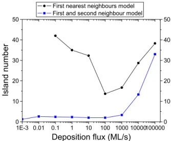
1E-3 0.01 0.1 1 10 100 1000 10000100000 0 10 20 30 40 50

First nearest neighbours model First and second neighbour model

Deposition flux (ML/s)

Is

land

number

0 10 20 30 40 50

Fig. 6. KMC simulations of graphene growth at T = 1273 K, with 2000 atoms (15% of a monolayer) deposited. Island number (excluding islands made of less than 20 atoms) in a simulation box of 80 × 160 atoms is given as a function of the depositionﬂux. The curve with black dots corresponds to simulations including nearest neighbours only (KMC 1), while the blue curve with square markers corresponds to the simulations that also include next nearest neighbours (KMC 2). (For interpretation of the references to colour in thisﬁgure legend, the reader is referred to the web version of this article.)

Fig. 5. KMC simulation of graphene growth at T = 1273 K, F0= 10−1ML/s and 2000 atoms

(15% of a monolayer) deposited, with next nearest neighbours accounted for (KMC 2). Red dots correspond to possible sites that can be occupied by carbon atoms, white dots are carbon atoms. (For interpretation of the references to colour in thisﬁgure legend, the reader is referred to the web version of this article.)

Fig. 4. KMC simulation of graphene growth at T = 1273 K, F0= 10−1ML/s and 2000 atoms

(15% of a monolayer) deposited only accounting for nearest neighbours (KMC 1). Red dots correspond to possible sites that can be occupied by carbon atoms, white dots are carbon atoms. (For interpretation of the references to colour in thisﬁgure legend, the reader is referred to the web version of this article.)

(6)

When counting only theﬁrst neighbours (KMC 1) we consider the following activation energies that account for the neighbours at the initial and_{ﬁnal position:}

EDiff¼ 0:5 eV ð4Þ

EDetach¼ 3:9 eV ð5Þ

EInc¼ 1:8 eV ð6Þ

EDec¼ 2:6 eV ð7Þ

EDiff is the activation energy for free diffusion or to attach to an island

(event 1 and reversed events 2, 3 and 5), EDetachthe energy when

going from two nearest neighbours to none (event 5), EIncthe activation

energy for going from one nearest neighbour to one or two neighbours (events 4 reversed and 6) and EDecis the activation energy to lose one

neighbour (events 2, 3 and 4). Even if the energy correspondence with the ab initio calculations is rather good (seeTable 1), we will see that this KMC 1 model does not reproduce the formation of large graphene islands. Theﬁrst neighbours are not sufﬁcient to simulate sp2 graphene, highlighting the importance of second nearest neighbours.

We then include next nearest neighbours (KMC 2). In this case, we have from 0 to 3 nearest neighbours and from 0 to 6 next nearest neigh-bours for each atomic site. Excluding atoms with 3 nearest neighneigh-bours that cannot move in our model, this gives a total of 21 possible con ﬁgu-rations if we consider only the initial position. Thus we cannot consider separately each diffusion process because of the time needed for the ab initio calculations and the complexity of the resulting KMC model and code. We keep one diffusion barrier EDifffor free diffusion or formation

of a C–C bond, an EIncbarrier for the increase of the number ofﬁrst

neighbours. All other events are described by a barrier Ebarthat depends

on the number of theﬁrst (nNN) and second (nNNN) nearest neighbours

associated with the diffusion. We have chosen the following energies to account for the ab initio data (Table 1):

EDiff¼ 0:5 eV ð8Þ

Ebar¼ nNNENNþ nNNNENNN ð9Þ

Einc¼ 1 eV: ð10Þ

The probability of detachment from an island is very important for theﬁnal shape of the island. Indeed, a very low probability of detach-ment leads to fractal shaped islands since no rearrangedetach-ment of the C

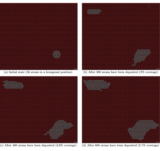
Fig. 8. Evolution of a KMC simulation of graphene growth at 1273 K, F0= 0.001 ML/s. Red dots correspond to possible sites that can be occupied by carbon atoms, white dots are carbon

(7)

atoms is possible, while the possibility of detachment leads to more compact shapes.

The values of ENN and ENNN were estimated from ab initio

calculations:

ENN¼ 1:3 eV; ð11Þ

ENNN¼ 0:6 eV: ð12Þ

When compared to the previous ab initio calculations, as seen in Table 1(KMC 2), the energy barrier is higher when detaching from one island to go to another island (event 4), and lower when dimers dissociate (event 2). Also, we do not include dimer diffusion, a diffusion event that has a rather high probability (ΔE ∼ 0.5 eV according to[42]), but we allow a relatively easy dissociation of dimers as a way of partly compensating this absence. The energy barrier for attachment is also higher, but it is still much lower than the barrier for detachment, so it has no signiﬁcant inﬂuence on the outcome of the simulations. The other barriers we use are all higher or equal to those found by ab initio, so our KMC model makes atoms slightly less likely to attach to other atoms, and slightly less likely to move once they are attached to another carbon atom. As we will see later, this will reduce the fragmentation of the islands. Additionally, the ab initio calculations include only a small number of atoms and probably underestimate the true energy barrier for diffusion from large islands.

Experimentally, graphene growth by CVD on copper has been report-ed for temperatures varying from 973 K to 1323 K[10,17]. Therefore, our simulations were done using a temperature of 1273 K, temperature for which most of the experimental results of the literature are found. The depositionﬂux we use is hard to relate to experimental parameters, but graphene coverage has been reported to increase from∼ 0.1 to ∼ 0.4 in about 600 s[17], leading to deposition rates of 5.10−4ML/s, though this rate is not constant and decreases over time. We model this decrease in deposition rate by rejecting deposition on sites that are already occupied by a carbon atom, but still taking into account this attempted deposition, as described previously (Fig. 3).

4. Results and discussion 4.1. KMC models compared

We_{first compare our two models: nearest neighbours only (KMC 1)} and also counting the second neighbours (KMC 2). The simulations where only thefirst nearest neighbours are counted result in very small islands (about 50–100 atoms) as an equilibrium shape for graphene flakes, seeFig. 4. This is true for various realistic parameter sets, and is incompatible with experimental evidence of larger islands of up to several μm[14]. The problem remains even if we take large islands as an initial condition as they tend to fragment into smaller ones.

To obtain bigger grapheneﬂakes, and to have a more realistic model of sp2_{graphene, we took into account the second nearest neighbours.}

We then obtained much larger islands (seeFig. 5). Actually taking into account the second nearest neighbours that tend to make atoms on the edge of islands more stable compared to atoms that attach to a small cluster explains the greater stability of large islands. This is not well reproduced in the ab initio simulations because only small islands have been considered.

Another illustration of this can be seen inFig. 6, which shows the number of islands in simulations including next nearest neighbours and excluding them. In both KMC models, wefind that the number of islands increases at very high depositionflux (36 islands at 100,000 ML/s inFig. 7for example, for KMC 2), which is expected in such simulations of 2D nucleation (see reference[43]): as higher depo-sitionfluxes result in less time for each atom to diffuse to an equilibrium position, this leads to atoms attaching quickly to small clusters. We also find that island number has a minimum around F = 100 ML/s for KMC

1. This is explained by large“fractal” islands forming when the deposi-tion rate is lowered; these islands then split up if the deposideposi-tion rate is lowered further before converging to an equilibrium size at very low deposition rates. In the case of KMC 2, island number falls low enough to have only one or two islands in each simulation. This means that the number of islands is not a statistically reliable parameter, but the trend of the formation of large islands will remain for larger systems. 4.2. Growth of graphene islands in KMC 2

Fig. 8shows a KMC 2 simulation of the evolution of graphene islands at 1273 K with a depositionﬂux of 0.001 ML/s. We can see an additional island nucleate inFig. 8b and both islands grow inFig. 8c and d. These islands, though small (about 300 atoms) are larger than most islands observed in the model including only nearest neighbours seen previously. Relatively small carbon clusters (21 or 24 atoms) are stable[44]and smaller than the islands weﬁnd in our simulations. We can expect our simulated islands to keep growing until they are of similar size to those seen in experiments. Our simulations with larger amounts of carbon deposited (4000 atoms instead of 2000) hint at this as islands keep grow-ing, and retain similar characteristics. From this we can conclude that our qualitative results for island shape and nucleation density can be extrap-olated to larger islands.

4.2.1. Qualitative effects of the depositionﬂux

Firstly, experimental results suggest that higher methaneﬂows lead to deviations from hexagonal shapes[19]and higher growth and nucleation rates. This is in perfect agreement with the relation we found between depositionﬂux and island shape.

Experiments have found that the pressure of hydrogen in the cham-ber is linked to the shape of the grapheneflakes, with increased hydro-gen pressures leading to more compact and hexagonalflakes[13,14,22]. Interpretations for the reasons of this effect differ. Vlassiouk et al. sug-gested a dual role of hydrogen,firstly as a cocatalyst for the formation of surface bound carbon species and, secondly, by etching away weaker carbon–carbon bonds[14]. Lewis et al.[22]have a similar interpretation. Wu et al. proposed that the presence of H2suppresses the decomposition

of methane on the copper substrate, which would slow the diffusion of carbon atoms on the surface through having CH4molecules as“obstacles”

to the diffusion of C atoms[13].

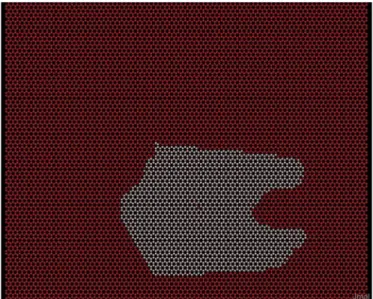
Fig. 9. KMC 2 simulation of graphene growth at T = 1273 K, F0= 10−3ML/s and 2000 atoms

(15% of a monolayer) deposited. Red dots correspond to possible sites that can be occupied by carbon atoms, white dots are carbon atoms. (For interpretation of the references to colour in thisﬁgure legend, the reader is referred to the web version of this article.)

(8)

Thefirst explanation supposes that hydrogen can etch away weak C–C bonds, which could be simulated by decreasing the energy barrier for the detachment of carbon atoms in our model. This is actually very similar to changing the depositionflux: when we reduce the deposition flux, weak C–C bonds have more time to be broken (strong C–C bonds are either very unlikely to be broken or impossible to break in the case of an entirely surrounded carbon atom).

Varying the value of the initial depositionﬂux F0causes qualitative

changes to the shape of the islands.Fig. 9shows an example of an island after deposition of 2000 carbon atoms at F0= 10−3ML/s and 1273 K,

whileFig. 5shows islands after deposition at F0= 0.1 ML/s, with all

other parameters constant. We see that the island formed during a low depositionﬂux is more compact and closer to a hexagon that the islands formed during a higher depositionﬂux.

This effect is not very surprising as a lower depositionﬂux supposes an increased time between the deposition of two atoms and therefore more time for the atom to reach an equilibrium position that is the more compact structure. Seen in another way, decreasing the deposi-tionﬂux leaves enough time for the system to evolve towards a more compact and hexagonal shape, seeFigs. 8 and 5, for example.

This point is conﬁrmed when considering the events that happen during simulations. For aﬂux of 105_{ML/s most of the events are free}

diffusion (the second most common event is two orders of magnitude less common), while at low diffusion (10−3ML/s) free diffusion is not even the most frequent event. Reducing the depositionﬂux causes the frequency of detachment events to increase, so the system evolves from a situation with almost no detachment to a situation where islands converge to equilibrium shapes because of the frequent attachment/ detachment processes.

As mentioned in the introduction of this article, in experiments an excessive amount of nucleation results in grain boundaries, once the islands have grown enough to merge. Grain boundaries are however not reproduced by our simulations as atoms occupy only fcc or hcp sites of the Cu (111) surface and can therefore not form topological defects.

In conclusion, our simulations reproduce the experimentally observed fact that a change in the rate of adsorption of the carbon atoms on the cop-per substrate is at the origin of a change of the shape of the carbon islands.

4.2.2. Island edge

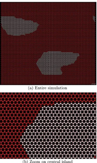
As seen previously, islands can be rather compact and hexagonal or be rather fractal. Yet in both cases“zigzag” edges tend to dominate, as can be seen inFig. 10.

This result is in agreement with previous experimental[14,35]and DFT[18]studies that found zigzag edges dominate. Armchair edges have been suggested to grow much faster than zigzag edges, which then causes the latter edges to be dominant[30]. Successive images of our simulations suggest that it is also the case in our model.

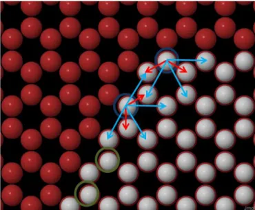
We explain it in the following way: we consider only the effect of the ﬁrst and second nearest neighbours and this has consequences when considering the difference between zigzag and armchair edges. Consid-ering only the edge of an island, visible inFigs. 11 and 12, only the edge atoms can move (the others have 3 nearest neighbours and are consid-ered immobile). In the case of the zigzag edge, there are 2 nearest neigh-bours and 4 next nearest neighneigh-bours. In the case of the armchair edge though, there are 2 nearest neighbours but only 3 next nearest neigh-bours. This means that, in our model, armchair edges are always less stable than zigzag edges. The same is true at angles between edges of different orientation.

Fig. 11. Neighbours in armchair edges. Selected atoms in green circles cannot move, red arrows showﬁrst nearest neighbours, blue arrows show second nearest neighbours. Red dots correspond to possible sites that can be occupied by carbon atoms, white dots are carbon atoms. (For interpretation of the references to colour in thisﬁgure legend, the reader is referred to the web version of this article.)

Fig. 10. KMC simulation of graphene growth at T = 1273 K, F=10−3ML/s and 2000 atoms (15% of a monolayer) deposited. Red dots correspond to possible sites that can be occupied by carbon atoms, white dots are carbon atoms. The edges of the island are mostly zigzag. Next nearest neighbours included (KMC 2). (For interpretation of the references to colour in thisﬁgure legend, the reader is referred to the web version of this article.)

(9)

5. Conclusion

This work set out to determine the morphology of grapheneﬂakes by using numerical simulations. Future experiments could then be guided and previous experimental results be explained, possibly allowing the adjustment of experimental parameters to improve graphene production. We used multiscale simulations, with fully quan-tum ab initio calculations for a few events and KMC simulations for large scale atomistic simulations. These two successive scales allowed us to take advantage of the speed of KMC algorithms and the precision from ﬁrst principles of the ab initio calculations.

Ab initio calculations were performed on graphene deposited on Cu (111) and diffusion barriers for carbon adatoms were determined. Events considered include free diffusion and attachment or detachment from graphene islands. Values of the diffusion barriers were often very different when reversing initial andﬁnal positions. We then developed an energy barrier model of the diffusion of carbon adatoms on Cu (111), based on results from ab initio calculations.

This model allowed us to observe the effect of deposition parameters on the initial states of the growth of grapheneflakes on Cu (111). We find that faster deposition of carbon atoms leads to shapes that are less hexagonal. These results were compared to some experimental data that have found both hexagons[13,14], multiple-lobed shapes[14], and even fractal shapes similar to snowflakes[13,45]. Our model is in qualitative agreement with these experimental reports. Our model also produces grapheneflakes on which zigzag edges dominate, providing a simple atomistic explanation to data reported in the literature.

Future improvements to the current model will involve simulating defects in the copper substrate, doping by other atoms such as nitrogen, and including multiple layers of graphene. This last point is challenging as the growth mode for additional layers is not currently well understood. Acknowledgments

The authors would like to thank J.-F. Colomer and N. Reckinger of the University of Namur for their valuable comments on the experimental

growth conditions. We would also like to thank A. L. Schoenhalz for her comments and criticism on this paper. The authors acknowledge the support of the Fonds De La Recherche Scientiﬁque - FNRS under convention 14571807 (doped graphene: multiscale simulations). This research used resources of the“Plateforme Technologique de Calcul Intensif” (PTCI) (www.ptci.unamur.be) located at the University of Namur, Belgium, which is supported by the Fonds De La Recherche Scientiﬁque - FNRS under convention No. 2.4520.11. The PTCI is a member of the“Consortium des Equipements de Calcul Intensif (CECI)” (www. ceci-hpc.be).

References

[1] K.S. Novoselov, Rev. Mod. Phys. 83 (2011) 837.

[2] C. Lee, X. Wei, J.W. Kysar, J. Hone, Science 321 (2008) 385.

[3] J. Nilsson, A. Neto, F. Guinea, N. Peres, Phys. Rev. Lett. 97 (2006).

[4] K.S. Novoselov, D. Jiang, F. Schedin, T.J. Booth, V.V. Khotkevich, S.V. Morozov, A.K. Geim, Proc. Natl. Acad. Sci. 102 (2005) 10451.

[5] C.-M. Seah, S.-P. Chai, A.R. Mohamed, Carbon 70 (2014) 1.

[6] X. Li, W. Cai, J. An, S. Kim, J. Nah, D. Yang, R. Piner, A. Velamakanni, I. Jung, E. Tutuc, S.K. Banerjee, L. Colombo, R.S. Ruoff, Science 324 (2009) 1312.

[7] L. Gao, W. Ren, H. Xu, L. Jin, Z. Wang, T. Ma, L.-P. Ma, Z. Zhang, Q. Fu, L.-M. Peng, X. Bao, H.-M. Cheng, Nat. Commun. 3 (2012) 699.

[8] R.S. Weatherup, B. Dlubak, S. Hofmann, ACS Nano 6 (2012) 9996.

[9] Q. Yu, L.A. Jauregui, W. Wu, R. Colby, J. Tian, Z. Su, H. Cao, Z. Liu, D. Pandey, D. Wei, T.F. Chung, P. Peng, N.P. Guisinger, E.A. Stach, J. Bao, S.-S. Pei, Y.P. Chen, Nat. Mater. 10 (2011) 443.

[10] H. Ago, Y. Ogawa, M. Tsuji, S. Mizuno, H. Hibino, J. Phys. Chem. Lett. 3 (2012) 2228.

[11] C. Mattevi, H. Kim, M. Chhowalla, J. Mater. Chem. 21 (2011) 3324.

[12] N. Reckinger, A. Felten, C.N. Santos, B. Hackens, J.-F. Colomer, Carbon 63 (2013) 84.

[13] B. Wu, D. Geng, Z. Xu, Y. Guo, L. Huang, Y. Xue, J. Chen, G. Yu, Y. Liu, NPG Asia Mater. 5 (2013) e36.

[14] I. Vlassiouk, M. Regmi, P. Fulvio, S. Dai, P. Datskos, G. Eres, S. Smirnov, ACS Nano 5 (2011) 6069.

[15] I. Vlassiouk, S. Smirnov, M. Regmi, S.P. Surwade, N. Srivastava, R. Feenstra, G. Eres, C. Parish, N. Lavrik, P. Datskos, S. Dai, P. Fulvio, J. Phys. Chem. C 117 (2013) 18919.

[16]L. Zhao, K. Rim, H. Zhou, R. He, T. Heinz, A. Pinczuk, G. Flynn, A. Pasupathy, Solid State Commun. 151 (2011) 509.

[17] H. Kim, C. Mattevi, M.R. Calvo, J.C. Oberg, L. Artiglia, S. Agnoli, C.F. Hirjibehedin, M. Chhowalla, E. Saiz, ACS Nano 6 (2012) 3614.

[18] Z. Luo, S. Kim, N. Kawamoto, A.M. Rappe, A.T.C. Johnson, ACS Nano 5 (2011) 9154.

[19] B. Wu, D. Geng, Y. Guo, L. Huang, Y. Xue, J. Zheng, J. Chen, G. Yu, Y. Liu, L. Jiang, W. Hu, Adv. Mater. 23 (2011) 3522.

[20] X. Li, C.W. Magnuson, A. Venugopal, R.M. Tromp, J.B. Hannon, E.M. Vogel, L. Colombo, R.S. Ruoff, J. Am. Chem. Soc. 133 (2011) 2816.

[21] J.M. Wofford, S. Nie, K.F. McCarty, N.C. Bartelt, O.D. Dubon, Nano Lett. 10 (2010) 4890.

[22] A.M. Lewis, B. Derby, I.A. Kinloch, ACS Nano 7 (2013) 3104.

[23] W. Zhang, P. Wu, Z. Li, J. Yang, J. Phys. Chem. C 115 (2011) 17782.

[24] H. Mehdipour, K.K. Ostrikov, ACS Nano 6 (2012) 10276.

[25] S. Karoui, H. Amara, C. Bichara, F. Ducastelle, ACS Nano 4 (2010) 6114.

[26] S. Haghighatpanah, A. Börjesson, H. Amara, C. Bichara, K. Bolton, Phys. Rev. B 85 (2012).

[27]S. Riikonen, A.V. Krasheninnikov, L. Halonen, R.M. Nieminen, J. Phys. Chem. C 116 (2012) 5802.

[28] H. Chen, W. Zhu, Z. Zhang, Phys. Rev. Lett. 104 (2010).

[29] X. Mi, V. Meunier, N. Koratkar, Y. Shi, Phys. Rev. B 85 (2012).

[30] H. Shu, X. Chen, X. Tao, F. Ding, ACS Nano 6 (2012) 3243.

[31] S. Lucas, P. Moskovkin, Thin Solid Films 518 (2010) 5355.

[32] P. Gaillard, J.-N. Aqua, T. Frisch, Phys. Rev. B 87 (2013).

[33] C.C. Battaile, Comput. Methods Appl. Mech. Eng. 197 (2008) 3386.

[34] T. Trevethan, C.D. Latham, M.I. Heggie, P.R. Briddon, M.J. Rayson, Nanoscale 6 (2014) 2978.

[35] J. Tian, H. Cao, W. Wu, Q. Yu, Y.P. Chen, Nano Lett. 11 (2011) 3663.

[36] G. Kresse, Phys. Rev. B 54 (1996) 11169.

[37] J. Paier, M. Marsman, K. Hummer, G. Kresse, I.C. Gerber, J.G. Ángyán, J. Chem. Phys. 124 (2006) 154709.

[38] P.E. Blöchl, Phys. Rev. B 50 (1994) 17953.

[39] J.P. Perdew, K. Burke, M. Ernzerhof, Phys. Rev. Lett. 77 (1996) 3865.

[40] T. Chanier, L. Henrard, Eur. Phys. J. B 88 (2015).

[41] P. Moskovkin, B. Bera, S. Lucas, NASCAM (2014) (www.unamur.be/sciences/physique/ pmr/telechargement/logiciels/nascamRetrieved on 14/12/2014.).

[42] O. Yazyev, A. Pasquarello, Phys. Rev. Lett. 100 (2008).

[43] A. Pimpinelli, J. Villain, Physics of Crystal Growth, Cambridge University Press, Cambridge, 1998.

[44] Q. Yuan, J. Gao, H. Shu, J. Zhao, X. Chen, F. Ding, J. Am. Chem. Soc. 134 (2012) 2970.

[45] E. Meca, J. Lowengrub, H. Kim, C. Mattevi, V.B. Shenoy, Nano Lett. 13 (2013) 5692.

Fig. 12. Neighbours in zigzag edges. Selected atoms in green circles cannot move, red arrows showﬁrst nearest neighbours, blue arrows show second nearest neighbours. Red dots correspond to possible sites that can be occupied by carbon atoms, white dots are carbon atoms. (For interpretation of the references to colour in thisﬁgure legend, the reader is referred to the web version of this article.)