RESEARCH OUTPUTS / RÉSULTATS DE RECHERCHE
Author(s) - Auteur(s) :
Publication date - Date de publication :
Permanent link - Permalien :
Rights / License - Licence de droit d’auteur :
Institutional Repository - Research Portal
Dépôt Institutionnel - Portail de la Recherche
researchportal.unamur.be
University of Namur
An iterative process for international negotiations on acid rain in Northern Europe
using a general convex formulation
Germain, Marc; Toint, Philippe
Published in:
Environmental and Resource Economics
DOI:
10.1023/A:1008301613492 Publication date:
2000
Document Version
Early version, also known as pre-print
Link to publication
Citation for pulished version (HARVARD):
Germain, M & Toint, P 2000, 'An iterative process for international negotiations on acid rain in Northern Europe using a general convex formulation', Environmental and Resource Economics, vol. 15, no. 3, pp. 199-216. https://doi.org/10.1023/A:1008301613492
General rights
Copyright and moral rights for the publications made accessible in the public portal are retained by the authors and/or other copyright owners and it is a condition of accessing publications that users recognise and abide by the legal requirements associated with these rights. • Users may download and print one copy of any publication from the public portal for the purpose of private study or research. • You may not further distribute the material or use it for any profit-making activity or commercial gain
• You may freely distribute the URL identifying the publication in the public portal ?
Take down policy
If you believe that this document breaches copyright please contact us providing details, and we will remove access to the work immediately and investigate your claim.
An iterative process for international negociations on acid rain in Northern Europe
using a general convex formulation
by M. Germain1, Ph.L. Toint2 and H. Tulkens3
Report 96/?? March 28, 1996
1 CORE, Universit´e Catholique de Louvain.
Email : [email protected]
2 Department of Mathematics, Facult´es Universitaires ND de la Paix,
61, rue de Bruxelles, B-5000 Namur, Belgium, EU Email : [email protected]
Current reports available by anonymous ftp from the directory “pub/reports” on thales.math.fundp.ac.be (internet 138.48.4.14)
3 CORE and IRES (Institut de Recherches Economiques et Sociales),
Universit´e Catholique de Louvain,
and Facult´es Universitaires Saint-Louis, Bruxelles Email: [email protected]
An iterative process for international negociations on acid rain in
Northern Europe using a general convex formulation
Marc Germain Philippe L. Toint Henri Tulkens March 28, 1996
Abstract
This paper proposes a dynamic game theoretical approach of international negociations on transboundary pollution. This approach is distinguished by a discrete time formulation (at variance with the continuous model of Kaitala et al., 1995) and by a suitable reformulation of the local information assumption on cost and damage functions: at each stage of the negoci-ation, the parties assign the best possible cooperative state, given the available informnegoci-ation, as an objective for the next stage. It is shown that the resulting sequences of states converges to a Pareto optimum in a finite number of stages. Furthermore, a financial transfer structure is also presented, which guarantees that the desired sequence of states is individually ratio-nal for the involved parties. The concepts are applied in a numerical simulation of the SO2
transboundary pollution problem related to acid rain in Northern Europe.
1
Introduction
Modelling international negociations on transboundary pollution has enjoyed a lot of attention in the recent past. Amongst the many contributions in this area, Chander and Tulkens (1991) present a general dynamic framework for such models, which is applied by Kaitala et al. (1995) in the context of the “acid rain game” in Northern Europe, that is the problem of negociating coordinated reductions in SO2 emission levels in Finland, Russia and Estonia. The framework
proposed by these authors does not assume that the information available to the negociating parties is global, as is for instance requested by M¨aler (1989) or Kaitala and Pohjola (1994), but rather supposes that this information is local in that it is limited to the marginal values of emission abatement costs and pollution damage costs to the environment, in a context where time is assumed to be continuous. Although an improvement on global information models, this proposal has the drawback that it requires, in theory, that the parties continuously negociate, a quite unrealistic situation.
Germain et al. (1996) reconsidered this framework and improved the realism in its represen-tation of time while suitably adapting the assumptions made on the local nature of information. More specifically, they assume that negociations are separated into well determined and distinct stages, and that the negociating parties know, at each stage, their emission abatement and dam-age cost function only up to certain thresholds determined by exogenous technological constraints.
At each stage, the parties then assign as a common objective the best cooperative state they can determine, given the available information. As these thresholds evolve with the progress made in reducing pollution, they show that the Pareto optimum is reached in a finite number of such negociation stages. Besides indicating that only a finite number of negociation stages is necessary to reach the optimum, their new approach has the advantage of clarifying the associated time scale, where negociations and periods between them are clearly distinguished.
However, as has been pointed out by Chander and Tulkens (1991) and Chander and Tulkens (1992), each of the negociating parties will continue to cooperate in such a process only if it finds cooperation individually profitable. Moreover, the stability of the program requires that none of the parties can find an advantage in abandonning it. These authors thus propose, in the context of their continuous model, a financial transfer technique ensuring that emission abatement costs are shared amongst all parties in such a way that all parties are induced to cooperate at each moment of time. Germain et al. (1996) manage to adapt Chander and Tulkens’s transfer scheme to their discrete dynamic process of negociation.
The present paper is mainly an extension of a previous report by the authors (see Germain et
al., 1996), where a similar model is presented and analyzed, but where different assumptions are
made on the form of the functions measuring the damage caused by pollution to the environment. While Germain et al. (1996) assume that this damage is linear in terms of the pollution levels, the present paper considers strictly convex damage functions. Because of the difficulty inherent in estimating these functions, it is indeed highly desirable to allow more than one representation. At variance with the linear case, we have to modify the equations for the financial transfers in order to apply them to the discrete case1. Since strictly convex damage functions no longer guarantee
strictly decreasing emission levels, the reasoning of Germain et al. (1996) leading to coalitional rationality is not applicable. This is why we now have to verify this property numerically. Finally, since the fact that some regions may be allowed to increase the pollutant emission levels may be difficult to accept for those who must reduce theirs, it seemed useful to simulate the cooperation process with the additional constraint that no increase in pollution level is permitted. This is an extension of the framework with linear damage functions, where this property automatically holds2.
2
The global problem and its approach in continuous time
The problem may be described as follows. There are n regions in which some atmospheric pollutant (such as SO2) is emitted with certain non-negative emission levels described by the
vector E = (E1, . . . , En)T. Once emitted, this pollutant is transported by winds between the
regions, this interregional transport being described by the n × n matrix A, whose i, j-th element aij ≥ 0 is the fraction of the pollutant emitted in region i and deposited in region j. If B is the
1This is notably different from the model introdoced by Kaitala et al. (1995), where the continuous time allow
direct application of Chander and Tulkens’s formula, irrespective of the linear or strictly convex nature of the damage functions.
n-vector of pollutant depositions with natural origin, the vector Q of total pollutant depositions in the n regions satisfies the relation
Q = Q(E) = AE + B, (2.1)
where A and B are supposed to be constant and exogenous. We assume that (2.1) holds at each moment in time, so that the fact that B is constant then implies that the pollutant does not accumulate in the regions.
Two cost functions are associated with each region. The first, denoted Ci(Ei), expresses the
emission abatement costs required by an emission level Ei in region i. We assume that Ci(·) is
decreasing for all positive emission levels Ei, which simply means that every emission reduction
generates costs for the emitting region. The second cost function, denoted Di(Qi), measures the
monetary value of the damage to the environment caused by a deposition Qi in region i. Ci(·)
and Di(·) are assumed to be continuous and convex. As a result, we may associate, with each
region, an aggregated cost function
Ji(E) = Ci(Ei) + Di(Qi(E)), (2.2)
where the depositions Qi(E) are given by (2.1).
The total cost for all regions is minimized by achieving the vector of emission levels E∗ = (E1∗, . . . , En∗)T obtained as solution of the program
min E J(E) def = n X i=1 Ji(E) (2.3)
such that (2.1) holds and
Ei≥ 0 (i = 1, . . . , n). (2.4)
E∗ is the vector of emissions at the Pareto optimum. Because of the convexity of the Ci(·) and
Di(·) this optimum is unique. The drawback of the program (2.3)+(2.1)+(2.4) is that it requires
that the cost functions Ci(·) and Di(·) are known for all possible values of their argument. This
can be unrealistic when the current emission levels and depositions are very different from the optimal ones: such an extensive knowldege of the cost functions may be very hard to obtain, or may be too unreliable to be used in effective interregional negociations.
Kaitala et al. (1995) propose3 to alleviate this difficulty by only assuming that the regions
know their cost functions locally, that is at the margin. It is then possible to define an emission reduction program governed by the differential system
dEi dt (t) = −K Ci′(Ei(t)) + n X j=1 ajiD′j(Qj(E(t))) , (i = 1, . . . , n), (2.5) 3
Following Tulkens (1979), whose model is inspired by the literature on “resource allocation processes” (Arrow and Hurwicz (1977), Malinvaud (1970) and Dr`eze and de la Vall´ee Poussin (1971)). All these processes are formulated in continuous time. Champsaur et al. (1977) have proposed a discrete time version which was found to be ill-adapted to the international problem considered here. This is why the present alternative process was developed.
where Ei(t) indicates that the emissions now depend on time (they are still related to the
de-positions by (2.1) with Q also depending on time), and where K is a positive constant. Be-cause the term between square brackets vanishes when the first order optimality conditions of (2.3)+(2.1)+(2.4) hold for strictly positive emission levels, it is possible to prove that these levels converge to their optimal values E∗
i, thus realizing Pareto optimum. The reader is referred to
Kaitala et al. (1995) for further details.
Although a clear improvement on assuming a global knowledge of the cost functions, this procedure remains problematic because it implies that an interregional negociation occurs at each moment in time, in order to ensure that (2.5) effectively governs the emission levels. This is of course impractical. Moreover, this approach has the further drawback that its time scale is not well defined as periods between two successive negociations are not modelled. Kaitala et al. thus propose to modify the dynamic of the process by adjusting the constant K to suit any specific time scale definition. This technique is interesting but does not resolve the difficulty that the time scale itself could be better defined. Our aim is to present, in the next section, an alternative dynamical model which does not suffer from these problems.
3
A discrete time approach with local information
At variance with the model described in the previous section, we now assume that negociation occurs at well defined times indexed by t = 0, 1, 2, . . .. The emission levels and depositions for the i-th region are thus given, at these times, by the quantities {Ei,t}∞t=0 and {Qi,t}∞t=0, where
(2.1) is assumed to hold for each time period, that is
Qt= Q(Et) = AEt+ B, (3.1)
(where Et = (E1,t, . . . , En,t)T and Qt = (Q1,t, . . . , Qn,t)T). In this notation, E0 and Q0 are the
initial emission levels and depositions before the first round of negociations. We also assume that the parties know their cost functions in a finite neighbourhood of the current emission levels and depositions, that is above a certain threshold strictly below these levels. Specifically, each region is assumed to know, for each period t, the values of the emission abatement cost Ci(Ei) for all
values of the emission levels
Fi,t ≤ Ei, (3.2)
where the lower bounds Fi,t satisfy the conditions 0 ≤ Fi,t< Ei,t for each i and each t. Similarly,
each region is assumed to know its damage function Di(Qi(E)) for each value of the vector of
emissions (E1, . . . , En)T above the same thresholds.
At the t-th negociation stage, the parties agree on a program to bring their emission levels from Et to the values Et+1 corresponding to a solution of the local optimization problem (2.3) in
the domain defined by the constraints (2.1) and (3.2)4. Once these emissions levels are attained, the bounds are updated to reflect the new information obtained during the period, according to Fi,t+1= min[Fi,t, τi,t+1Ei,t+1] (3.3)
4Note that J(·) is the sum of convex function and is therefore convex. Hence the local problem (2.3)+(2.1)+(3.2)
for i = 1, . . . , n, where
0 ≤ τi,t+1≤ τ (3.4)
for some constant 0 ≤ τ < 1. The procedure may then be repeated for the (t + 1)-th negociation stage. Of course, it may well happen that Et+1= Etfor some t, in which case no further action is
requested from the parties and the procedure is then terminated. Note that (3.3) ensures that the domains defined by the constraints (3.2) for successive t are nested, and hence that termination occurs at stage t if Ei,t > Fi,t for all i.
One then has the following important result, which states that the emission levels (and hence depositions) converge to a state corresponding to a Pareto optimum, provided the level set
L0 def
= {E | J(E) ≤ J(E0) and Ei feasible (i = 1, . . . , n)} (3.5)
is bounded. This assumption is fairly weak. It is for instance satisfied if the emission levels are not only non-negative but also bounded above (a very plausible situation), or if
lim kEk→∞ n X i=1 Di(Qi(E)) = ∞. (3.6)
This latter condition is also natural in our context, since it only reflects the fact that increasing pollutant emission cause increased damage, maybe not locally, but somewhere within the regions under consideration.
Theorem 1 Under the conditions stated above, the sequence {Et} generated by the procedure
converges to a solution of the problem (2.3)+(2.1)+(2.4). Furthermore, this convergence occurs in a finite number of stages if all limiting values of the emissions are all strictly positive.
The interested reader is referred to Germain et al. (1996) for a proof.
4
An application to Northern European negociations about
acid rain
We now examine the impact of the model and theory developed in the previous section on the ”acid rain game” in Northern Europe. Specifically, the problem is for Finland (divided in three regions), three regions of Russia and Estonia to agree on a program for reducing SO2 emissions,
which should limit acid rain and its associated damages5. The emission abatement costs are
assumed to be, in the interval [0, ˜Ei], of the form
Ci(Ei) = γi+ αi( ˜Ei− Ei) + βi( ˜Ei− Ei)2 (4.1)
for each i = 1, . . . , n while the damage functions may be written as Di(Qi) = 1 2πiQ 2 i (4.2) 5
for each i. Both these costs are expressed in millions of 1987 Finnish Marks (MFIM) and the depositions are expressed in thousands of tons per year (KT/Y). The parameters αi, βi, γi, πi
and ˜Ei are positive. Their values, together with those of B and the initial levels E0, Q0 in 1987,
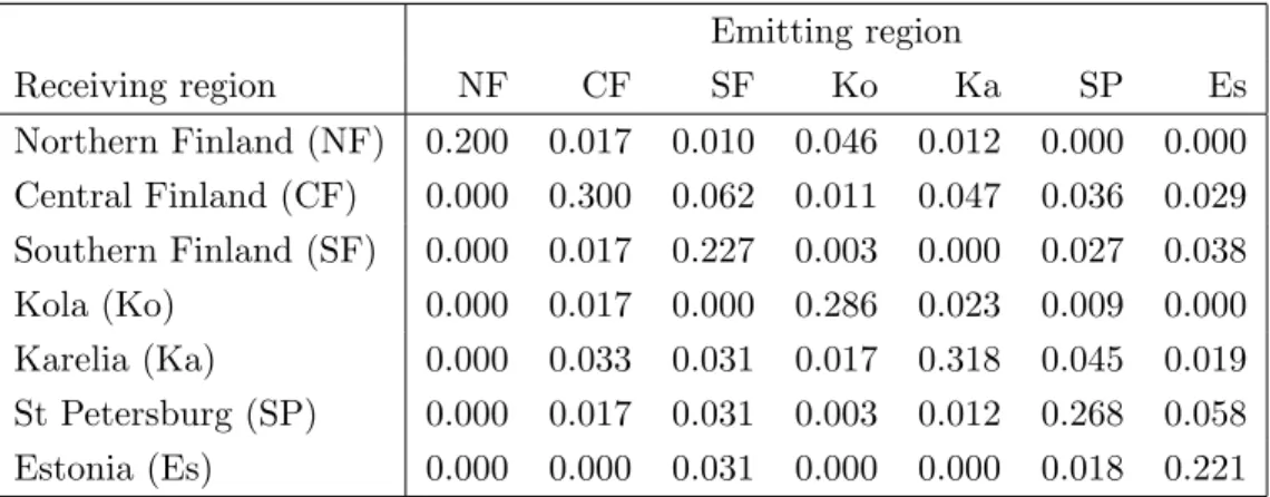
are given in Table 1. The initial state is the same as that considered by Kaitala et al. (1995) and Germain et al. (1996), which is that of a Nash equilibrium between Finland (with its three regions merged) and the USSR of 1987 (whose four regions are also merged). The transport coefficients (the matrix A) is given in Table 2. The information thresholds for the costs and damage functions are determined using the formula (3.3) where τi,t = 0.95 for all i and t, which
means that these functions are known for all emission levels above 95% of the current ones.
i Region Ei,0 Qi,0 Bi αi βi γi E˜i πi
1 Northern Finland 5 46 26 10.0 2.093 5.9 5 1.09 2 Central Finland 60 98 59 3.8 0.172 33.0 60 0.09 3 Southern Finland 97 66 35 4.6 0.068 53.6 97 0.24 4 Kola: 350 131 27 0.02 • 98 ≤ E4 ≤ 350 1.0 0.000 0.0 350 • 0 ≤ E4 ≤ 98 1.0 0.077 252.0 98 5 Karelia 85 95 50 4.0 0.045 0.0 85 0.12 6 St Petersburg 112 88 46 6.0 0.051 0.0 112 0.22 7 Estonia: 104 60 32 0.05 • 60 ≤ E7 ≤ 104 2.0 0.000 0.0 104 • 0 ≤ E7 ≤ 60 2.0 0.191 88.0 60
Table 1: Parameters and initial levels
Emitting region Receiving region NF CF SF Ko Ka SP Es Northern Finland (NF) 0.200 0.017 0.010 0.046 0.012 0.000 0.000 Central Finland (CF) 0.000 0.300 0.062 0.011 0.047 0.036 0.029 Southern Finland (SF) 0.000 0.017 0.227 0.003 0.000 0.027 0.038 Kola (Ko) 0.000 0.017 0.000 0.286 0.023 0.009 0.000 Karelia (Ka) 0.000 0.033 0.031 0.017 0.318 0.045 0.019 St Petersburg (SP) 0.000 0.017 0.031 0.003 0.012 0.268 0.058 Estonia (Es) 0.000 0.000 0.031 0.000 0.000 0.018 0.221
Table 2: Transport coefficients in 1987
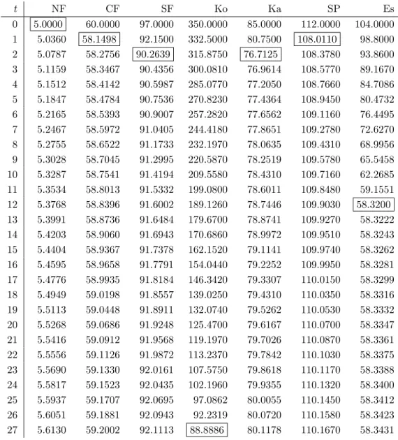
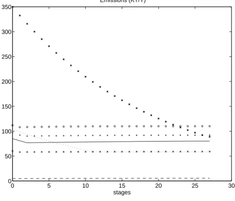
Table 3 and Figure 1 show the evolution of the SO2 emission levels that result from the
procedure described in the previous section. In the figure (and all following ones), the regions are identified as follows: Northern Finland’s trajectory is represented by a dashed line, Central
Finland’s by “x” Southern Finland’s by “+”, Kola by stars, Karelia’a by a continous line, St Petersburg by circles and Estonia by a dotted line. The final state (t = 27) is the Pareto optimum for the problem and corresponds to that reported by Kaitala et al. (1995). The numerical computations were performed by using the LANCELOT package for nonlinear optimization by Conn et al. (1992). t NF CF SF Ko Ka SP Es 0 5.0000 60.0000 97.0000 350.0000 85.0000 112.0000 104.0000 1 5.0360 58.1498 92.1500 332.5000 80.7500 108.0110 98.8000 2 5.0787 58.2756 90.2639 315.8750 76.7125 108.3780 93.8600 3 5.1159 58.3467 90.4356 300.0810 76.9614 108.5770 89.1670 4 5.1512 58.4142 90.5987 285.0770 77.2050 108.7660 84.7086 5 5.1847 58.4784 90.7536 270.8230 77.4364 108.9450 80.4732 6 5.2165 58.5393 90.9007 257.2820 77.6562 109.1160 76.4495 7 5.2467 58.5972 91.0405 244.4180 77.8651 109.2780 72.6270 8 5.2755 58.6522 91.1733 232.1970 78.0635 109.4310 68.9956 9 5.3028 58.7045 91.2995 220.5870 78.2519 109.5780 65.5458 10 5.3287 58.7541 91.4194 209.5580 78.4310 109.7160 62.2685 11 5.3534 58.8013 91.5332 199.0800 78.6011 109.8480 59.1551 12 5.3768 58.8396 91.6002 189.1260 78.7446 109.9030 58.3200 13 5.3991 58.8736 91.6484 179.6700 78.8741 109.9270 58.3222 14 5.4203 58.9060 91.6943 170.6860 78.9972 109.9510 58.3243 15 5.4404 58.9367 91.7378 162.1520 79.1141 109.9740 58.3262 16 5.4595 58.9658 91.7791 154.0440 79.2252 109.9950 58.3281 17 5.4776 58.9935 91.8184 146.3420 79.3307 110.0150 58.3299 18 5.4949 59.0198 91.8557 139.0250 79.4310 110.0350 58.3316 19 5.5113 59.0448 91.8911 132.0740 79.5262 110.0530 58.3332 20 5.5268 59.0686 91.9248 125.4700 79.6167 110.0700 58.3347 21 5.5416 59.0912 91.9568 119.1970 79.7026 110.0870 58.3361 22 5.5556 59.1126 91.9872 113.2370 79.7842 110.1030 58.3375 23 5.5690 59.1330 92.0161 107.5750 79.8618 110.1170 58.3388 24 5.5817 59.1523 92.0435 102.1960 79.9355 110.1320 58.3400 25 5.5937 59.1707 92.0695 97.0862 80.0055 110.1450 58.3412 26 5.6051 59.1881 92.0943 92.2319 80.0720 110.1580 58.3423 27 5.6130 59.2002 92.1113 88.8886 80.1178 110.1670 58.3431
Table 3: Evolution of the SO2 emissions
As show by Table 3, 27 negociation stages are necessary, given our assumptions, to reach the optimum. This number of stages could of course be reduced if the values chosen for τi,t
were smaller. If we now compare the initial and final states, we note that the reductions vary considerably between regions. While the emissions of Central and Southern Finland, Karelia and St Petersburg are slightly reduced, the reduction is much more substantial for Kola and Estonia. We even note the remarkable increase for Northern Finland. A similar situation occured in
0 5 10 15 20 25 30 0 50 100 150 200 250 300 350 stages Emissions (KT/Y)
Figure 1: Evolution of the SO2 emissions
Kaitala et al. (1995), where it is explained as follows. Observe that, at the Nash equilibrium, the marginal emission abatement costs Ci′ in the various regions are quite different from each other: some may be very high, as is precisely the case with Northern Finland. Observe also that the sum of marginal damagesPn
j=1ajiπjQj being now an increasing function of the depositions,
decreases with the reduction of the latter. Therefore, at some stage t and for some region i, the sum of marginal damages becomes equal to its marginal emission abatement cost (implying ∆Ei = 0 for this i), while such equality does not (yet) hold for the other regions j 6= i. The
reduction in depositions achieved by these other regions then induce a decrease ofPn
j=1ajiπjQj
while Ci′ does not change, thus inducing a sign reversal in ∆Ei.
Table 3 also shows that, with the exception of Kola, none of the regions which, in fine, reduce their emission levels, do so monotonically. The boxed entries in Table 3 indicate, for each region, the minimum emission reductions achieved in the process. Northern Finland is at its minimum at the initial state, Central and St Petersburg achieve it at the first stage, Central Finland and Karelia at the second, Estonia at the twelfth and Kola at the final stage only. That some regions do increase their emissions after this minimum has been reached may again be explained as above, noting that the steady decrease in Kola’s emissions induces a decrease in depositions in the whole area, implying in turn a decrease in marginal damage and hence raising the depollution opportunity in several regions.
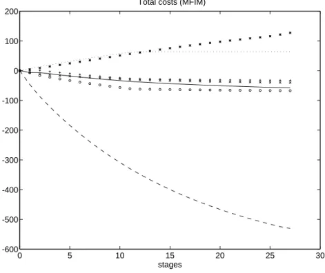
equilibrium to the final Pareto optimum. More precisely, we report in Table 4 the values Ji(E∗) − Ji(E0) = Ci(E∗) − Ci(E0) + Di(E∗) − Di(E0)
for i = 1, . . . , n, where E∗ is the optimal emission level reached at stage 27. The table also reports the same costs aggregated for the whole of Finland, the whole of the three regions of Russia and Estonia. Figure 2 presents the evolution of these costs over the 27 negociations stages.
Finland Russia Estonia
NF CF SF Ko Ka SP Es
-530.34 -40.07 -32.78 127.33 -57.50 -67.35 63.65
-603.19 2.48 63.65
Table 4: Total costs (Ji(E∗) − Ji(E0)) per region and country (MFIM)
0 5 10 15 20 25 30 -600 -500 -400 -300 -200 -100 0 100 200 stages Total costs (MFIM)
Figure 2: Evolution of the total costs per region
These results show that the emission reduction program does considerably profit to Finland, but costs to Russia and even more to Estonia. The cooperation of these two countries in such a program is thus unlikely, unless some financial transfers can be defined between the regions, that would compensate for these incurred costs. The definition of such a strategy is the object of the next section.
5
Cooperation and financial transfers
The main idea is that the aggregated reduction of total costs J(E0) − J(E∗) (also called the
“ecological surplus”) can be used as a resource to share between the regions in order to induce their cooperation within the emission reduction program. This surplus is, in the example of the previous section, equal to 537 MFIM per year, that is 13.9% of the initial total cost, a very respectable amount. It is more than sufficient to offer to Russia and Estonia a financial transfer that would reduce their costs below the level supported initially, while maintaining considerable advantages for the other regions.
However, the surplus J(E0) − J(E∗) is only known at the end of the reduction program, once
the emission levels E∗ are achieved. Thus it cannot be used in any practical negociation process between the parties during the program. Instead, one needs a key to share whatever benefit are achieved at a given negociation stage between the regions, in order to ensure that each of them continues to cooperate within the program. The aim of this section is to show that such financial transfers can indeed be found.
Let us start from the fact that the total surplus obtained between two negociation stages is the sum of the different regions’ gains or losses, that is
∆Jt= Jt+1− Jt= n X i=1 ∆Ji,t = n X i=1 [∆Ci,t+ ∆Di,t]. (5.1)
Because of the quadratic form of the damage function (4.2), we obtain that ∆Di,t≤ n X j=1 ∂Di ∂Ej (Ej,t+1)[Ej,t+1− Ej,t] = πiQi,t+1 n X j=1 aij∆Ej,t. (5.2)
Combining (5.1) and (5.2), we see that ∆Jt ≤ n X i=1 ∆Ci,t+ n X i=1 πiQi,t+1 n X j=1 aij∆Ej,t = n X j=1 [∆Cj,t+ ∆Ej,t n X i=1 aijπiQi,t+1] def = n X j=1 ∆Gj,t, (5.3)
defining the ∆Gj,t. These quantities can be seen as a linear approximation of the total surplus
obtained when region j decreases its emissions6.
We have now the following result.
Theorem 2 At each stage t of the negociation process and for all regions (j = 1, . . . , n), one has that
∆Gj,t≤ 0 and ∆Rj,t ≤ 0, (5.4)
where ∆Gj,t is defined in (5.3) and
∆Rj,t def = ∆Dj,t− πjQj,t+1 n X i=1 aji∆Ei,t. (5.5) 6
When time is continuous (as in Kaitala et al., 1995) or when the damage functions are linear (as in Germain et al., 1996), inequalities in (5.2) and (5.3) are replaced by equalities, and ∆Gj,t is then exactly the total surplus due to ∆Ej,t.
Proof. For stage t, consider the functions Gj(Ej) def = Cj(Ej) + Ej n X i=1 aijπiQi,t+1, j = 1, ..., n,
where Qi,t+1 are considered as parameters. This definition implies that
∆Gj,t= Gj(Ej,t+1) − Gj(Ej,t) (5.6)
because of (5.3), and the convexity of Gj in Ej also yields that
Gj(Ej,t+1) − Gj(Ej,t) ≤ G′j(Ej,t+1)[Ej,t+1− Ej,t]. (5.7)
Now, the derivative of Gj is given by
G′j(Ej) = Cj′(Ej) + n
X
i=1
aijπiQi,t+1
and the first order optimality conditions of problem (2.3)-(2.1)-(3.2) at stage t + 1 imply that G′j(Ej,t+1) = Cj′(Ej,t+1) + n X i=1 aijπiQi,t+1≥ 0 (5.8) when Ej,t+1 ≤ Ej,t and G′j(Ej,t+1) = Cj′(Ej,t+1) + n X i=1 aijπiQi,t+1= 0 (5.9)
otherwise, because the emissions are only bounded from below. Combining (5.6), (5.7), (5.8) and (5.9) then yields the first part of (5.4).
Moreover, we have, from (5.5), that ∆Jt− n X j=1 ∆Gj,t= n X j=1 ∆Dj,t− n X j=1 ∆Ej,t n X i=1 aijπiQi,t+1= n X i=1 ∆Ri,t. (5.10)
The second part of (5.4) then follows from (5.2). ✷
Using this result, we may then specify for each region i and each negociation stage t, a financial transfer Ti,t (negative if received by i or positive if paid) given, for i = 1, . . . , n, by
∆Ti,t = −∆Ci,t− ∆Di,t+
X
j
δij,t[∆Gj,t+ ∆Rj,t], (5.11)
where
0 ≤ δij,t≤ 1, ∀i, j, t and n
X
i=1
δij,t= 1, ∀j, t. (5.12)
The first two terms of (5.11) are equivalent to levy on region i its gain on total cost, while the third term corresponds to returning to the region a fraction δij,tof each of the surpluses ∆Gj,t+ ∆Rj,t.
One immediately verifies that the budget of these transfers is balanced at each period, namely that
n
X
i=1
Moreover, as the total cost for region i with transfers is JT
i = Ci(Ei) + Di(Ei) + Ti, (5.14)
we have then that
∆JiT = ∆Ci+ ∆Di+ ∆Ti = n
X
j=1
δij,t[∆Gj,t+ ∆Rj,t] ≤ 0, (5.15)
for i = 1, ..., n, because of (5.4). In other words, the total cost of each region decreases at each negociation stage. This property, called individual rationality, provides a minimum cooperative character to the sequence of negociations.
Of course, conditions (5.12) do not define the transfers in a univoque manner. All matrices of positive parameters δij,t whose columns sum up to one are adequate. Following Chander and
Tulkens (1991) and Germain et al. (1996), we propose to choose δij,t= ∂Di/∂Ej Pn k=1∂Dk/∂Ej = aijD ′ i(Qi,t) Pn k=1akjDk′(Qk,t) . (5.16)
These values verify (5.12) and thus ensure the properties of balanced budget (5.13) and individual rationality (5.15). With linear damage functions, Chander and Tulkens (1991) have managed to derive certain results of coalition rationality, ensuring that there is no advantage for a coalition of regions to form and cooperate in a framework more restricted than the full inter-regional cooperation considered here. Unfortunately, extending these results in the quadratic case is not easy. We will therefore not insist on this interpretation of (5.16), but rather postpone this discussion for the future. We have however verified numerically that coalition rationality holds for our example if the full information is available (τ = 0).
6
The transfers in the example
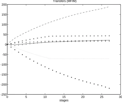
The application of formulae (5.13) and (5.16) to the cooperation problem between Finland, Russia and Estonia leads to the evolution of transfers illustrated by Figure 3. Recall that Ti,t ≥ 0(≤ 0)
means that region i pays (receives) transfers. Estonia and Kola are the principal recipients of transfers, i.e. the regions that reduce most their emissions and whose global costs without transfers increase with international cooperation (see Figure 2). The principal payer is Northern Finland, the region that profits most from cooperation. Figure 3 also shows that Southern Finland and Karelia benefit marginally of transfers during the first stages, but they soon become payers, as St. Petersburg and Northern and Central Finland.
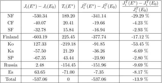
The presence of transfers doesn’t imply that the benefits of cooperation are evenly distributed among regions, as shown (in absolute terms) by the third column of Table 57. The fact that
the total cost of each region decreases illustrates the property of individual rationality of the negociation process with transfers. The last column of Table 5 shows that the distribution of the surplus is also uneven in relative terms. Because of its low initial costs (due to its very low marginal damage), Kola obtains, taking the transfers into account, the most important relative reduction of total costs, followed by Northern Finland.
7
0 5 10 15 20 25 30 -250 -200 -150 -100 -50 0 50 100 150 200 stages Transfers (MFIM)
Figure 3: Evolution of the transfers per region
At the national level, one observes that Russia is nearly indifferent to collaboration. Despite of this, its share of the transfers is more favourable than for Estonia. Due to the complex dependance of the δij,t on the transport and damage coefficients and on the deposit levels (see
(2.1), (4.2) and (5.16)), it is difficult to clarify each of these elements’ influence on the evolution of transfers. It appears however that the damage coefficient of Estonia (π7, given by Table 1)
is much smaller than those of Karelia and St. Petersburg. On the other hand, optimal deposits are lower in Estonia than in Karelia and St. Petersburg (about 60%) and comparable to Kola’s. Given (5.13) and (5.16), these two elements may partly explain in why transfers go mainly to Russia rather than to Estonia.
7
Monotonicity constraint on the emissions
As noted in Section 4, emissions do not decrease monotonically to the optimum. In the case of Northern Finland, emissions even grow (see Table 3). For psychological reasons, the fact that certain regions may increase their emissions can be unacceptable for those who must reduce them. For this reason, we have revisited the exercise of Sections 4 and 6 with the additional requirement that no emission is allowed to increase from one stage to the next. Of course, the Pareto optimum may not be attainable when such monotonicity constraints are imposed, but we note that the sequence of negociation stages is still well defined, and also that the financial transfers remain
Ji(E∗) − Ji(E0) Ti(E∗) JiT(E∗) − JiT(E0) JT i (E∗) − JiT(E0) JT i (E0) NF -530.34 189.20 -341.14 -29.29 % CF -40.07 20.41 -19.66 -4.23 % SF -32.78 15.84 -16.94 -2.93 % Finland -603.19 225.45 -377.74 -17.12 % Ko 127.33 -219.18 -91.85 -53.45 % Ka -57.50 21.29 -36.26 -6.69 % SP -67.35 43.44 -23.90 -2.80 % Russia 2.48 -154.45 -151.96 -9.69 % Es 63.65 -71.00 -7.35 -8.17 % Total -537.06 0 -537.06 -13.9 %
Table 5: Reduction cost figures without (column 1) and with transfers (column 3) (MFIM).
computable and still satisfy (5.13) and (5.15)8. Results for the constrained case are presented in
Tables 6 and 7.
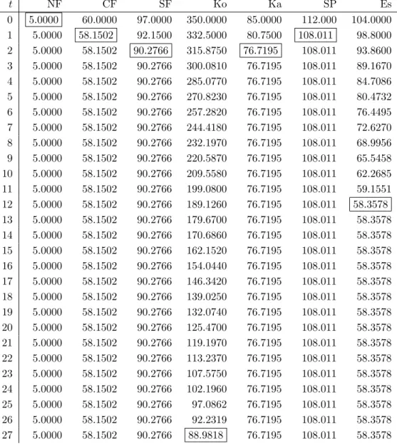
Table 6 indicates the evolution of emissions to the new constrained optimum. The boxed entries indicate that each region attains its target at very different times. By comparison with Table 3, it appears that
• the number of stages to get to the global optimum is the same;
• emissions of a given region are minimum at the same time, the difference being that they now remain there, because of the monotonicity constraint;
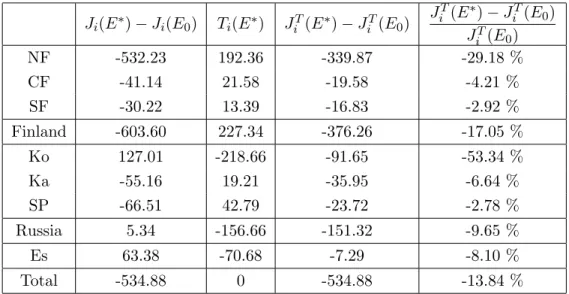
• optimal emission levels are lower, except for Kola and Estonia whose levels are identical. In other words, regions tend to depollute to much in comparison with the free optimum. Comparison of Tables 5 and 7 leads to the conclusion that differences are minimal. Without transfers (column 1), some regions may be better off when emissions are constrained to be mono-tone than in the unconstrained situation (Northern Finland, Central Finland, Kola and Estonia), even if of course the global surplus is smaller. On the other hand, when transfers are taken into account (column 3), all regions loose a little compared with the first exercise. This leads to the conclusion that, if the monotonicity constraint may improve the political aspects of the successive negociations stages, its introduction does not lead to substantial or qualitative perturbations.
8
Indeed, while G′
j(Ej,t+1) ≤ 0 when the upper bound on the emissions of region j is active, the fact that
t NF CF SF Ko Ka SP Es 0 5.0000 60.0000 97.0000 350.0000 85.0000 112.000 104.0000 1 5.0000 58.1502 92.1500 332.5000 80.7500 108.011 98.8000 2 5.0000 58.1502 90.2766 315.8750 76.7195 108.011 93.8600 3 5.0000 58.1502 90.2766 300.0810 76.7195 108.011 89.1670 4 5.0000 58.1502 90.2766 285.0770 76.7195 108.011 84.7086 5 5.0000 58.1502 90.2766 270.8230 76.7195 108.011 80.4732 6 5.0000 58.1502 90.2766 257.2820 76.7195 108.011 76.4495 7 5.0000 58.1502 90.2766 244.4180 76.7195 108.011 72.6270 8 5.0000 58.1502 90.2766 232.1970 76.7195 108.011 68.9956 9 5.0000 58.1502 90.2766 220.5870 76.7195 108.011 65.5458 10 5.0000 58.1502 90.2766 209.5580 76.7195 108.011 62.2685 11 5.0000 58.1502 90.2766 199.0800 76.7195 108.011 59.1551 12 5.0000 58.1502 90.2766 189.1260 76.7195 108.011 58.3578 13 5.0000 58.1502 90.2766 179.6700 76.7195 108.011 58.3578 14 5.0000 58.1502 90.2766 170.6860 76.7195 108.011 58.3578 15 5.0000 58.1502 90.2766 162.1520 76.7195 108.011 58.3578 16 5.0000 58.1502 90.2766 154.0440 76.7195 108.011 58.3578 17 5.0000 58.1502 90.2766 146.3420 76.7195 108.011 58.3578 18 5.0000 58.1502 90.2766 139.0250 76.7195 108.011 58.3578 19 5.0000 58.1502 90.2766 132.0740 76.7195 108.011 58.3578 20 5.0000 58.1502 90.2766 125.4700 76.7195 108.011 58.3578 21 5.0000 58.1502 90.2766 119.1970 76.7195 108.011 58.3578 22 5.0000 58.1502 90.2766 113.2370 76.7195 108.011 58.3578 23 5.0000 58.1502 90.2766 107.5750 76.7195 108.011 58.3578 24 5.0000 58.1502 90.2766 102.1960 76.7195 108.011 58.3578 25 5.0000 58.1502 90.2766 97.0862 76.7195 108.011 58.3578 26 5.0000 58.1502 90.2766 92.2319 76.7195 108.011 58.3578 27 5.0000 58.1502 90.2766 88.9818 76.7195 108.011 58.3578
Table 6: Evolution of the SO2 emissions with monotonicity constraints
8
Conclusion
We have proposed and analyzed a dynamic cooperation process to reduce transboundary pol-lution between several countries or regions. This process ensures that the Pareto optimum is attained in a finite number of negociation stages, each consisting of a period of negociation on the emission reductions, based on limited information, followed by a period during which emis-sions are effectively reduced. We have also shown that international financial transfers can be found, ensuring that costs of reduction are distributed in such a way that cooperation is profitable for each region. If emissions are prevented from increasing at any stage, one furthermore observes that the final state may be very near the free optimum.
Ji(E∗) − Ji(E0) Ti(E∗) JiT(E∗) − JiT(E0) JT i (E∗) − JiT(E0) JT i (E0) NF -532.23 192.36 -339.87 -29.18 % CF -41.14 21.58 -19.58 -4.21 % SF -30.22 13.39 -16.83 -2.92 % Finland -603.60 227.34 -376.26 -17.05 % Ko 127.01 -218.66 -91.65 -53.34 % Ka -55.16 19.21 -35.95 -6.64 % SP -66.51 42.79 -23.72 -2.78 % Russia 5.34 -156.66 -151.32 -9.65 % Es 63.38 -70.68 -7.29 -8.10 % Total -534.88 0 -534.88 -13.84 %
Table 7: Ultimate reduction cost figures without (column 1) and with transfers (column 3) under the monotonicity constraint (MFIM)
further developments. First, the interval of time between two stages of negociation is currently exogenous and could be integrated in the objective. Secondly, the thresholds up to which the abatement and damage cost functions are known could be considered as part of the negociation process itself. A strategic analysis would in this respect complete classical work on revealed preferences and costs. Finally, the analysis could be extented to pollution stock problems, where permanent effects of depositions are present. This would require to reformulate the objective in intertemporal terms. One can find an interesting such attempt in M¨aler (1992).
References
[Arrow and Hurwicz, 1977] K. J. Arrow and L. Hurwicz, editors. Studies in Resource Allocation
Processes, Cambridge, UK, 1977. Cambridge University Press.
[Champsaur et al., 1977] P. Champsaur, J. Dr`eze, and C. Henry. Stability theorems with eco-nomic applications. Econometrica, 45(2):273–294, 1977.
[Chander and Tulkens, 1991] P. Chander and H. Tulkens. Strategically stable cost sharing in an economic-ecological negociation process. In K. G. M¨aler, editor, International Environmental
Problems, Dordrecht, NL, 1991. Kluwer Academic Publishers. (to appear).
[Chander and Tulkens, 1992] P. Chander and H. Tulkens. Theoretical foundations of negociations and cost sharing in transfrontier pollution problems. European Economic Review, 36(2/3):288– 299, 1992.
[Conn et al., 1992] A. R. Conn, N. I. M. Gould, and Ph. L. Toint. LANCELOT: a Fortran package
for large-scale nonlinear optimization (Release A). Number 17 in Springer Series in
Computa-tional Mathematics. Springer Verlag, Heidelberg, Berlin, New York, 1992.
[Dr`eze and de la Vall´ee Poussin, 1971] J. Dr`eze and D. de la Vall´ee Poussin. A tˆatonnement process for public goods. Review of Economic Studies, 38:133–150, 1971.
[Germain et al., 1996] M. Germain, Ph. Toint, and H. Tulkens. Calcul ´economique it´eratif pour les n´egociations internationales sur les pluies acides entre la Finlande, la Russie et l’Estonie.
Annales d’Economie et de Statistique, (to appear), 1996.
[Kaitala and Pohjola, 1994] V. Kaitala and M Pohjola. Acid rain and international environmental aid: A case study of transboundary pollution between Finland, Russia and Estonia. In K. G. M¨aler, editor, International Environmental Problems, Dordrecht, NL, 1994. Kluwer Academic Publishers.
[Kaitala et al., 1995] V. Kaitala, K. G. M¨aler, and H. Tulkens. The acid rain game as a resource allocation process, with application to negociations between Finland, Russia and Estonia. The
Scandinavian Journal of Economics, (to appear), 1995.
[M¨aler, 1989] K. G. M¨aler. The acid rain game. In H. Folmer and E. Van Ierland, editors,
Valuation Methods and policy Making in Environmental Economics, Amsterdam, NL, 1989.
Elsevier.
[M¨aler, 1992] K. G. M¨aler. Critical loads and international environmental cooperation. In R. Pethig, editor, Conflicts and cooperation in managing environmental resources, pages 71–81, Berlin, 1992. Springer Verlag.
[Malinvaud, 1970] E. Malinvaud. Procedures for the determination of a program of collective consumption. European Economic Review, 2:187–217, 1970.
[Tulkens, 1979] H. Tulkens. An economic model of international negotiations relating to trans-frontier pollution. In K. Krippendorf, editor, Communication and Control in Society, pages 199–212, New York, 1979. Gordon and Breach Science Publishers.