HAL Id: tel-03022147
https://tel.archives-ouvertes.fr/tel-03022147
Submitted on 24 Nov 2020HAL is a multi-disciplinary open access archive for the deposit and dissemination of sci-entific research documents, whether they are pub-lished or not. The documents may come from teaching and research institutions in France or abroad, or from public or private research centers.
L’archive ouverte pluridisciplinaire HAL, est destinée au dépôt et à la diffusion de documents scientifiques de niveau recherche, publiés ou non, émanant des établissements d’enseignement et de recherche français ou étrangers, des laboratoires publics ou privés.
Analysis by “reverse engineering” methods of ultra-table
piezoelectric resonators and noise modelling.
Alok Pokharel
To cite this version:
Alok Pokharel. Analysis by “reverse engineering” methods of ultra-table piezoelectric resonators and noise modelling.. Vibrations [physics.class-ph]. Université Bourgogne Franche-Comté, 2020. English. �NNT : 2020UBFCD025�. �tel-03022147�
THESE DE DOCTORAT DE L’ETABLISSEMENT
UNIVERSITE BOURGOGNE FRANCHE-COMTE
PREPAREE A L’UNIVERSITE DE FRANCHE-COMTE
Ecole doctorale n°37
ED SPIM
Doctorat de Sciences pour l’Ingénieur
Par
M. POKHAREL Alok
Analyse par des méthodes de “reverse engineering” de résonateurs piézoélectriques
hautes performances et modélisation du bruit.
Analysis by “reverse engineering” methods of ultra-table piezoelectric resonators
and noise modelling.
Thèse présentée et soutenue à Besançon, le 10 Septembre 2020.
Composition du Jury :
M. PRIGENT Michel Professeur des Universités, XLIM, IUT du Limousin, Limoge, Président M. CILIBERTO Sergio Directeur de Recherche, CNRS, ENS Lyon, Rapporteur M. LLOPIS Olivier Directeur de Recherche, CNRS, LAAS, Toulouse, Rapporteur M. DEVEL Michel Professeur des Universités, FEMTO-ST, ENSMM, Besançon, Examinateur M. VOROBYEV Nicolas Ingénieur CNES, Toulouse, Examinateur M. IMBAUD Joël Maître de Conférences, FEMTO-ST, ENSMM, Besançon, Codirecteur de thèse M. STHAL Fabrice Professeur des Universités, FEMTO-ST, ENSMM, Besançon, Directeur de thèse
Dédicace À mes Parents. À mon frère. À Elina.
IV
ACKNOWLEDGEMENTS
It is a privilege and honour to receive the constant support of all the members of FEMTO-ST and ENSMM throughout the period of my thesis to achieve this dream of my life. I will always remain grateful and indebted for their valuable support through the course of this dissertation.
This thesis work would not have been possible without the financial support of “Région Bourgogne Franche-Comté” and the LABEX Cluster of Excellence FIRST- TF (ANR-10-LABX-48-01) for supporting this thesis work in their program “Investissement d’Avenir” operated by French National Research Agency (ANR). I would like to thank CNES for providing resonators for my thesis work and to the project supported by ANR ASTRID titled ECLATEMPS (Etude de Cristaux de LGT pour Applications Temps-Fréquence) (ANR-12-ASTR-0030-01) for providing LGT resonators. I am also thankful to FEMTO-ST department of Time and Frequency and ENSMM and to l’École Doctorale SPIM for all the follow-ups and support during the 4 years period.
I would like to express my humble gratitude to my thesis advisor Professor Fabrice Sthal for his guidance and patience towards me throughout the period of this thesis. His motivation, encouragement, being up-to-date and a sense of “proving by doing” role was an unimaginable base to help me focus on my work. Similarly, I feel grateful to thank my co-advisor Associate Professor Joël Imbaud whose perspective I admire in starting to do a work little by little as commendable throughout the journey of my thesis. Together with this, I am very much thankful to Joël for some of the experimental part of my thesis.
I thank Professor Michel Devel for his high-level expertise in helping me understand the theoretical part of my thesis. His ideas were a boon to find a solution for modelling phase noise from a statistical perspective and along with this my gratitude for accepting to report on this thesis. Also, I would like to thank Professor Célestin C. Kokonendji from Laboratoire de Mathématiques de Besançon, for his presentations in understanding stable distributions.
I would like to thank the jury members Sergio Ciliberto, Directeur de Recherche in CNRS, Laboratoire de Physique de l’ENS Lyon and Olivier Llopis, Directeur de Recherche in CNRS-LAAS, Toulouse.
I would like to thank Michel Prigent, Professeur des Universités from XLIM, IUT du Limousin, Limoge and Nicolas Vorobyev, Ingénieur at CNES from Toulouse to examine this work.
I equally thank Serge Galliou (ex-director) and Yann Kersalé (current director) of FEMTO-ST, department of Time and Frequency for allowing me to work in the lab during my thesis period.
I thank Sarah and Fabienne at FEMTO-ST, department of Time and frequency for their sincere administrative help. Not to forget Clara Lahu from HR department, ENSMM and Alika Rossetti from UBFC SPIM for their administrative and scholarly help during my thesis.
V
I would also thank David Vernier for his active help in providing me electronic equipment for LabView tutorials and Phillippe Abbé for all the technical help in the lab regarding electronics and mechanics.
I would also like to thank my cool colleagues Etienne and Jérémy, with whom I had a chance to have a humorous time and not a single working day was there where we did not pass out jokes or made fun of something. I am thankful for an exciting unplanned trip with Guillaume, Sabina, and Giacomo to Colmar and Abondance, it was really an awesome moment. I thank Alexandre (an office mate and a friend with a big sound...Ha!Ha!Ha!), together we had an amazing trip to Orlando, Miami, and Tampa. I also thank Anthony my colleague during the end year of my thesis, Rémy a cool sportive friend and Melvin, Gregoire, François, Stefania, Gauthier, Kevin, Falzon with whom I passed memorable times of my life. I also thank the newcomers Arthur, Tung, Isha, Merieme and Shambo with whom I had a wonderful time.
I would also like to thank my family members for providing me all the emotional support during the period of my thesis.
VII
TABLE OF CONTENTS
ACKNOWLEDGEMENTS ... IV GENERAL OVERVIEW ... XI
Chapter 1 Introduction ... 1
1.1 The world of Quartz Crystal ... 1
1.1.1 Why do we need quartz ... 2
1.1.2 History of innovation of quartz that led to its usage ... 2
1.1.3 Quartz used in resonators ... 3
1.2 BAW resonator ... 4
1.2.1 Equivalent circuit of a resonator ... 4
1.2.2 Realisation of Q factor in BAW resonators ... 8
1.2.3 Relationship between Q-factor and temperature ... 9
1.2.4 Governing tensor equations of continuum mechanics for a piezoelectric material ... 10
1.3 Background of BAW resonators in FEMTO-ST ... 15
1.4 Basics in Metrology ... 16
1.5 Statistical method of generalizing frequency fluctuations ... 19
1.5.1 Power Spectral Density (PSD) ... 19
1.5.2 Different kinds of intrinsic noises in the electronic system ... 21
1.6 Fluctuations measuring basics in Time domain and Frequency domain ... 23
1.6.1 Time domain characteristics ... 23
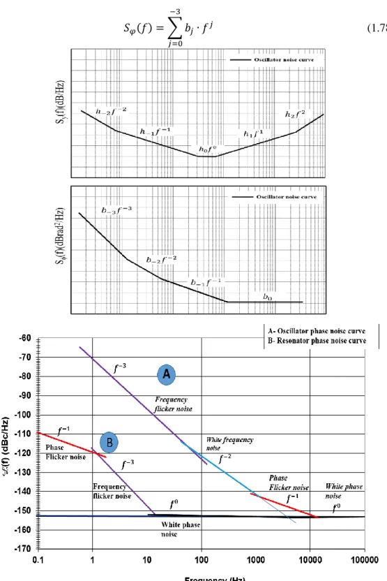
1.6.2 Frequency domain characteristics ... 23
1.7 Leeson’s effect for Phase noise in resonator ... 26
1.8 Summary ... 29
Chapter 2 Noise measurement technic ... 31
2.1 Phase noise measurement using Carrier Suppression Technic ... 31
2.2 Phase Noise Measurement Technic in BAW resonators ... 32
2.2.1 Measurement of the Inversion Point Temperature and Motional Parameters ... 32
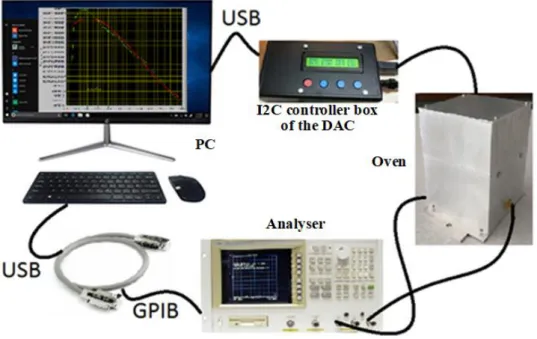
2.2.2 Identification of Resonator Pins ... 33
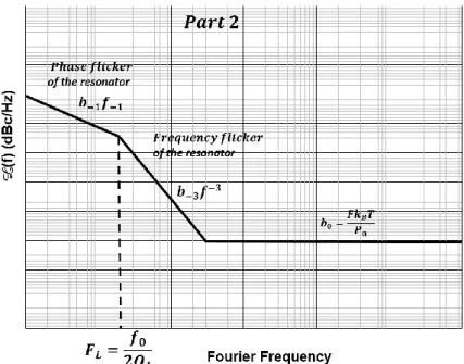
2.2.3 Internal and external structure of the oven and components used ... 34
2.2.4 The value calibration of the thermostat ... 35
2.3 Preparation of resonator for phase noise measurements ... 36
2.3.1 Phase noise measurement bench using carrier suppression technic ... 37
2.3.2 Calibration of the carrier suppression technic ... 39
2.3.3 Example of phase noise measurement on Quartz resonators ... 40
2.4 Improved phase noise measurement technic on Langatate resonators ... 41
VIII
2.4.2 Study of phase noise of Langatate crystal resonators ... 42
2.4.3 LGT resonator parameters ... 43
2.4.4 Phase noise measurement with special adaptation circuit ... 45
2.4.5 Pspice introduction, modelling, and simulation ... 46
2.5 Phase noise measurement results of LGT resonators ... 48
2.5.1 Measurement of noise floor ... 48
2.5.2 Measurement of phase noise in LGT resonators ... 49
2.6 Summary ... 50
Chapter 3 Noise measurement on quartz crystal resonators to explain 1/f noise ... 52
3.1 1/f phase noise measurement in bulk acoustic wave resonators... 52
3.2 Principle or energy trapping – Stevens and Tiersten model of infinite plate resonators ... 52
3.2.1 For an infinite plate ... 52
3.2.2 Energy trapping in electrodes ... 56
3.2.3 Stevens – Tiersten plano-convex model ... 57
3.3 Modelisation of SC- cut BAW quartz crystal resonator using Tiersten’s model ... 59
3.3.1 Investigation of flicker noise of ultra-stable quartz crystal resonator ... 59
3.3.2 Instability in Quartz crystal resonator ... 61
3.4 Experimental results on phase noise measurement in BAW resonators ... 64
3.5 Finite Element Method (FEM) analysis ... 71
3.6 Simulation results and comparison with Tiersten’s model ... 73
3.7 Summary ... 75
Chapter 4 Experimental attempts at checking a theoretical model for 1/f phase noise ... 77
4.1 Introduction ... 77
4.2 Modelling background ... 79
4.2.1 Stable distributions ... 79
4.2.2 One sided α -stable distribution and Cahoy’s formula ... 84
4.2.3 Mittag-Leffler functions and distributions ... 87
4.2.4 Non-exponential relaxation ... 91
4.2.5 Intermittency ... 93
4.3 Observation and test of Markus Niemann et al.’s model on 1/f fluctuations in quartz resonators ... 95
4.3.1 Definition of Niemann et al.’s model and notations ... 95
4.3.2 Experimental setup ... 97
4.3.3 Preliminary results for a series of 48 phase noise measurements for a good-average quartz crystal resonator pair ... 99
4.3.4 Results for series of 101 phase noise measurements in various ultra-stable quartz crystal resonator pairs ... 100
IX
4.3.5 Tests on the possibility to model 1/f phase noise in the ultra-stable quartz crystal
resonators using Mittag-Leffler or one sided α-stable distributions ... 105
4.4 Summary ... 108
Chapter 5 Quartz crystal resonator in reverse engineering ... 110
5.1 Analysis of the quartz crystal resonator by reverse engineering ... 110
5.2 Bulk acoustic wave cavity quartz crystal resonators at room temperature and constraints 111 5.3 Dismantling the quartz crystal resonator ... 111
5.4 Defects in the quartz crystal material ... 113
5.4.1 Chemical impurities ... 113
5.4.2 Inclusions ... 113
5.4.3 Dislocations ... 114
5.5 X-rays diffraction Topography ... 115
5.5.1 Production of X-rays ... 116
5.5.2 Principle of production of X-rays ... 116
5.5.3 Anticathodes ... 116
5.5.4 X-rays generator ... 117
5.5.5 Absorption of X-rays ... 117
5.5.6 Coefficient of absorption of X-rays ... 117
5.5.7 X-rays transmission technic used in FEMTO-ST ... 118
5.6 Quartz crystal block and cutting ... 121
5.7 X-rays Tomography ... 122
5.8 Laser scattering ... 124
5.8.1 Scattering ... 125
5.8.2 Reflection ... 125
5.8.3 Diffraction ... 125
5.9 Experimental laser setup in FEMTO-ST... 126
5.10 Summary ... 126
Conclusion ... 128
Annexes ... 132
A. Piezoelectric effect in Quartz and IEEE norms ... 132
B. Numerical values of the components of material tensors for quartz ... 135
References ... 137
List of figures ... 150
XI
GENERAL OVERVIEW
The continued research on quartz crystals has led to the optimization of piezoelectric resonators used in devices in the time and frequency domain. Their applications were initially limited to military devices, but they can now be found in many different electronic devices available for the public.
A crystal resonator is specified to operate at a given (resonance) frequency, within a given temperature range for best results, and under severe conditions of vibrations over a long period. The equations of motion of quartz representative volume elements, incorporating piezoelectric effects, allow us to find resonance frequencies and their corresponding modes of vibrations as a function of orientation of the resonator axes with respect to the crystallographic axes. The BAW (Bulk Acoustic Wave) quartz crystal resonators used for this thesis can operate at three different modes of vibration i.e. extension-compression mode A, fast shear mode B and slow shear mode C. The inversion point temperature of this kind of resonator with an SC (Stress Compensated) cut vibrating at 3rd overtone mode-C is around 80-85° C. For this kind of resonator, the quality factor is in order of two and half millions at 5 MHz resonant frequency.
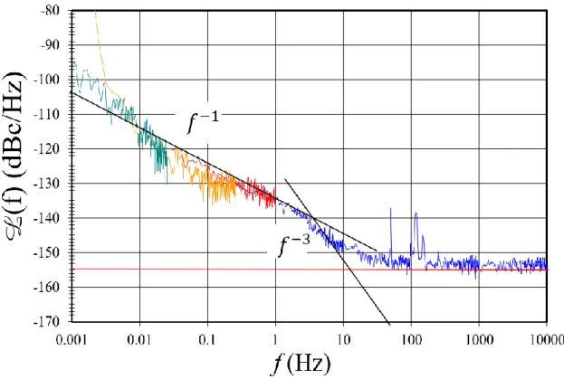
Applications of this kind of resonators are quite common in metrological systems (atomic clocks in GNSS satellite positioning devices) for a frequency range between 0.8 MHz and 200 MHz. The best BAW resonators can have a short-term relative stability in time of about 10-14 at room temperature, so that they are termed as “ultra-stable”. Researches are still going on to try to improve that stability value or prove that it is an intrinsic material limit and find all the factors affecting it. We know that the short-term stability of an oscillators built from a resonator is dependent on the quality factor (loaded) of the resonator which itself depends on the quality of the material, but also that it is not the only driving factor. The fundamental origin of this stability limit is still unknown, but we can study limiting factors through their impact on the random fluctuations in frequency and phase of the resonator output signal (frequency noise or phase noise). This kind of work has been carried out, for years, in the Time and Frequency department at FEMTO-ST (and its LPMO and LCEP ancestors), notably through the development of a state of the art comparison technique to measure the noise in resonators from BAW resonators (5 MHz - 5 GHz). In this PhD thesis, we mainly concentrated on the study of the low frequency part of the Power spectral density of phase noise which is roughly inversely proportional to the inverse of the frequency shift with respect to the resonance frequency used (commonly known as “1/f noise” or “flicker noise” in the quartz crystal resonator community).
Following previous works in FEMTO-ST in collaboration with CNES and several other European partners, a large quantity of very high performance 5 MHz ultra-stable SC-cut quartz crystal resonators were provided for reverse engineering during this thesis work. Here, “reverse engineering” should be understood like “going back to the cause of the problem by dismantling the resonators and characterizing their parts”. Along with this, resonators fabricated from other piezoelectric materials
XII
such as LGT (Langatate) have also been used. Hence, comparative investigations were carried out to study the influence of the type of material and crystallographic defects, on 1/f phase noise in acoustic resonators.
Thesis organisation:
The work carried out in this thesis has been organised into five chapters as:
• Chapter 1 begins with a brief description of quartz as a piezoelectric material, equivalent electrical circuit of quartz, governing equations in quartz, a short background on the quartz resonators used for this thesis and their possible use in metrological devices. Then, detailed information regarding the different kinds of noise in resonators are given, with equations that are used in all the succeeding chapters.
• Chapter 2 focuses on the technical part of this thesis. It introduces a unique phase noise measurement technic used for acoustic quartz resonators in FEMTO-ST. This chapter includes all the necessary details required for setting up and using the phase noise measurement bench. Similarly, it also details the alternative phase noise measurement technic used for low motional resistance resonators i.e. LGT resonators. Finally, the chapter concludes with results of some phase noise measurements using these classical and alternative phase noise measuring technics. • Chapter 3 deals with the study of propagation of acoustic waves in a plano-convex shaped quartz crystal resonator. The work starts with the definition of an infinite piezoelectric plate as a theoretical basis to introduce the concept of energy trapping in a quartz resonator. The chapter further gives core details of modelling of a plano-convex resonator with electrodes using Stevens and Tiersten’s model and implements all the tensor equations necessary for the design as derived in Chapter one. Similarly, the frequencies of overtones and anharmonic modes of the 5 MHz SC-cut plano-convex resonators along with the frequency-temperature effects occurring in them are determined. Then, we discuss results of phase noise measurement in plano-convex quartz resonators at two different temperatures i.e. 353K and 4K. The classification of our resonators according to their short-term stability values (good, average, or bad) and their Q-factors is then discussed. Finally, we validate the Stevens and Tiersten’s model using the Finite Element Method as implemented in COMSOL – Multiphysics, for most of the visible modes of vibration for mode-C.
• Chapter 4 presents result of statistical tests that we performed on series of 101 phase noise measurements at 353K on the same resonator pairs. More precisely, after providing some background information on some peculiar statistical distributions of probability known as stable distributions and Mittag-Leffler distributions, we briefly review the main ideas of several papers that use them for the modelling of some physical processes that happen during relaxation
XIII
of a short perturbation imposed to the system, using statistical thermodynamics. We then give account of tests of intermittency as a possible physical origin of 1/f noise in our resonator, using Mittag-Leffler distribution and conclude with discussing the fits of the distribution of the 101 relative PSD of noise averaged over the frequency interval in which the 1/f modelisation is appropriate.
• In Chapter 5, we describe the analysis performed on dismantled good and bad resonators as part of a “reverse engineering” program which is a crucial work for this thesis. Photographs of the internal part have been taken by a high definition camera from different angles. This allowed us to see the defects visible to the naked eye on the mounting, on the electrodes and on the crystal itself. Further, to see the intrinsic crystal defects i.e. dislocations and inclusions, X-rays diffraction and laser scattering have been used, respectively.
1
Chapter 1 Introduction
From more than half a century, resonators have been serving in time and frequency applications as the popular and simpler piezo-electronic device. The piezo-electronic device consists of piezoelectric material for e.g. Quartz, Langatate (La3Ga5.5Ta0.5O14), Gallium orthophosphate (GaPO4) etc., dimensioned, oriented according to their crystallographic axes, and equipped with a pair of conducting electrodes. Vice versa, these electrodes excite the resonator into mechanical vibration because of piezoelectric effect. The result is that, a resonator behaves like a R-L-C circuit composed of a resistor, inductor, and capacitor. This leads the vibrational energy to be minimum except when the frequency of the driving field is in the periphery of one of the normal modes of vibration “energy trapping” and resonance occurs.
As the fact of today, different piezoelectric materials are on investigation for resonator characteristics, but for many years, quartz resonators had been preferred in satisfying needs for precise frequency control and selection. Compared to other piezoelectric resonators, like, those made from ceramics and single-crystal materials, quartz resonators have unique combination of properties. The materials properties of quartz are both extremely stable and highly repeatable from one specimen to another. Likewise, the acoustic loss of the quartz resonator is particularly low, leading directly to one of the key properties of resonators i.e. high Quality (Q) factor. Its intrinsic Q is around 2.7 ∙ 106 at 5 MHz. Therefore, this low loss factor and frequency stability of resonators make quartz the most sought-after material in designing and manufacturing ultra-stable high frequency resonators.
1.1 The world of Quartz Crystal
Materials used for acoustics are usually characterised by the elastic linearity, high quality factor i.e. Q, zero temperature coefficients (ZTCs) of frequency, and more precisely by the presence of piezoelectricity. Piezoelectricity has many benefits like, mechanism of efficient transduction between mechanical motion and electrical variables. Similarly, the compensation of stress and temperature transient, evolved from non-linearities is possible with quartz, making available high stability bulk acoustic wave (BAW) resonators and the Surface Acoustic Waves (SAW) resonators, which provides conveniently accessible time axes for signal processing operations like convolution [1]. Whereas, from the application point of view, for several oscillator applications, the piezoelectric coupling 𝑘 need not to be large. The reason is that, the operating point of an oscillator confines to the resonator inductive region where a small coupling resembles a narrow inductive range, and high oscillator stability.
Modern-day applications in acoustics include devices like, wireless transceivers for voice, data, internets, Wireless Local Area Networking (WLAN) including WLAN robot, timing and security applications, Code Division Multiple Access (CDMA) filters, non-volatile memories, and micro-electromechanical (MEMS)/ micro-optomechanical (MOMS) devices. Some of the SAW applications are analog signal processing (convolvers, duplexers, delay lines, and filters), for the mobile
2
telecommunications, multimedia, and Industrial-Scientific-Medical (ISM) bands, wireless passive identification tags, sensors, transponders, and microbalances. BAW applications include resonators in precision clock oscillators, front-end GPS filters for cell phones, thin-films, solidly mounted resonators (SMRs), and stacked crystal filters (SCFs) formed as SMRs, for integration with microwave heterojunction bipolar transistors (HBTs).
1.1.1
Why do we need quartz
The answer, quartz is the only known material that possess the following combination of properties [1]:
• Piezoelectric (as the whole world knows!). • Zero temperature coefficient cuts.
• Stress/thermal transient compensated cuts. • High acoustic Q and naturally low loss.
• Capable of withstanding 35,000-50,000 g shocks. • Very stable.
• Capable of integrating with micro and nano-electronic components.
• Easy to process, hard but not brittle, under normal conditions, low solubility in everything except fluoride etchants.
• Abundance in nature: it is easy to grow in large quantities, at low cost, and with high purity and perfections. Data from 2015 A.D shows that, fabricated crystal makes up to 3,769 tonnes per year and is second only to silicon.
1.1.2
History of innovation of quartz that led to its usage
History of innovation of quartz summarises below [1]:1800-1900s- Piezoelectric effects discovered by Brothers Pierre and Jacques Curie; first hydrothermal growth of quartz in Lab was possible.
1910- 1920s- First quartz crystal oscillator and first quartz crystal-controlled clock was developed. 1930-1940s- Temperature compensated BAW AT/BT cuts developed.
1950- 1960s- Quartz bars were commercially viable; theory of vibration of anisotropic plates were proposed.
1960-1970s- “Energy trapping” theory came in to play to reduce unwanted modes; surface acoustic wave (SAW) cuts; temperature compensated ST was developed; stress compensated (SC) compound cut developed; BVA resonators were fabricated; cryo-pumps were proposed.
1980-1990s- Stress-compensated BAW compound cut (SBTC) developed; thin-film resonators realized; solidly mounted resonators fabricated.
3
1.1.3
Quartz used in resonators
Quartz has always been a most common material used for fabricating resonators. In the beginning, natural quartz has a long history of use to fabricate resonators, but later, because of high purity, low production costs and easy handling, synthetic crystals took over the market for resonator fabrication. However, today, the use of natural quartz has been limited for the fabrication of pressure transducers in deep wells.
We can use any object made of elastic material, possibly as a crystal because all the materials have natural resonant frequency of vibrations. Just take an example of material like steel, which is very elastic and has a high speed of sound. In fact, in mechanical filters, people used steels before quartz. Today, a properly cut and mounted quartz can distort in the electric field supplied by the electrodes on the crystal. Hence, when the field removed, the quartz generates the electric field and returns to the previous shape. Nevertheless, the advantage of using the material quartz is the presence of its elastic constants where its size changes in a way to maintain the frequency dependence on temperature to be very low. However, the temperature specific characteristics depends on the mode of vibration and the angle of quartz cut. This is advantageous because the resonant frequency of the plate depends on its size and does not change much. Some of the popular modes of vibrations are in Figure 1.1.
Figure 1.1: Different modes of vibration used in resonator fabrication [2].
The benefit of using different modes of vibration is that, the fabrication of different sized resonators and oscillators been made possible as can be seen in Figure 1.2 and Figure 1.3 respectively. However, to be specific, we do not intend to establish all the historical advancement of quartz resonators and oscillator except for few already mentioned above; rather, the purpose of showing different kinds of resonators and oscillators in Figure 1.2 and Figure 1.3 is to picturize how the technology has made the adaptation of quartz crystals to the small electronic devices.
4
Figure 1.2: Different kinds of fabricated resonators [2].
Figure 1.3: Small-sized oscillator fabricated using quartz crystal [2]. Major real-life usages of quartz are given in Table 1.1 [1]:
Aerospace Research/metrology Industry Consumer Automotive
Communications Atomic clocks Telecom Watches/clocks Engine control
Navigation Instruments Aviation Cell phones Trip computer
Radar Astronomy Disk drives Radio/Hi-Fi GPS
Sensors Space tracking Modems Colour TV
Guidance Celestial
investigation
Computers Pacemakers
Warfare Digital systems VCR/Video
camera Table 1.1: Table of quartz uses in different domains.
1.2 BAW resonator
1.2.1
Equivalent circuit of a resonator
The circuit in Figure 1.4 is an electrical equivalent circuit for a quartz crystal resonator where 𝐶0 is the parasitic capacitance that accounts for all the stray capacitive effects in the circuit. The motional parameters 𝐶1, 𝑅1 𝑎𝑛𝑑 𝐿1 are the capacitance, resistance, and inductance respectively in series. When this circuit extends as, 𝐶𝑛, 𝑅𝑛, 𝑎𝑛𝑑 𝐿𝑛 , each series arm accounts for one resonance and represents the overtones or harmonics of that resonant frequency as shown in Figure 1.5.
5
Figure 1.4: a. Mechanical-Electrical equivalent, b. Crystal unit symbol, c. Electrical [3] equivalent circuit.
Figure 1.5: Extended equivalent circuit with overtones.
Further, the extended circuit resembles three families of motion namely Mode-A- longitudinal mode, Mode-B- fast shear mode and Mode-C- slow shear mode, as in Figure 1.6., for an anisotropic material.
Figure 1.6: Equivalent circuit resembling three families of motion.
As a first approach, we assume that no external forces act on our resonator system except the damping. The governing differential equation derived from Newton’s second law of motion for ‘free and damped’ vibration will be:
𝑚𝑢"+ 𝛾𝑢′+ 𝑘𝑢 = 0 (1.1)
Where, 𝑚 is the mass, 𝑢 is the displacement of the mass from an equilibrium position, 𝛾 is the viscous damping coefficients and 𝑘 is the spring constant and are all positive. Upon solving for the roots of the characteristic equation above, we get:
6 𝑟1,2=
−𝛾 ± √𝛾2− 4𝑚𝑘
2𝑚 (1.2)
Moreover, the three possible cases are critical damping 𝛾 = 2√𝑚𝑘 = 𝛾𝐶𝑅, over damping 𝛾 > 2√𝑚𝑘 and under damping 𝛾 < 2√𝑚𝑘. Then equation (1.1) will be:
𝑚𝑢"+ 2𝜁𝜔
0𝑢′+ 𝜔02𝑢 = 0 (1.3)
Where, 𝜔0= √ 𝑘
𝑚 is the natural frequency of resonance i.e. the resonant frequency, 𝜁 = 𝛾
𝛾𝐶𝑅 is the damping ratio and 𝛾𝐶𝑅 = 2√𝑚𝑘 is the critical damping ratio. For the under-damping case where 𝜁 < 1, the roots of the characteristic equation will be complex of the form 𝑟1,2= 𝜆 ± µ𝑖. For the underdamped case, given the equation of harmonic vibration by 𝑢 = 𝐴𝑒𝑗𝛺𝑡, the frequency 𝛺 will be a complex pair, one of them being:
𝛺 = 𝜔0√1 − 𝜁2 +𝑖𝜔0 𝜁 Or 𝛺 = 𝜔𝑅𝑒+ 𝑖𝜔𝑖𝑚 (1.4) Where 𝜔𝑅𝑒 and 𝜔𝑖𝑚 are the real and imaginary part of the frequencies.
The damping of the displacement 𝑢 measures as: 𝛿 = 2𝜋𝜁
√1−𝜁2 = 2𝜋𝜔𝑖𝑚
𝜔𝑅𝑒 (1.5)
Which clearly helps us to calculate the Quality factor 𝑄 as the inverse of the damping, given by: 𝑄 =1
𝛿 = 𝜔𝑅𝑒
2𝜋𝜔𝑖𝑚 (1.6)
Where 𝛿 = 2𝜋𝜁 from equation (1.5) and (1.6), and 𝑄 can be written as: 𝑄 = 1
2𝜁 Or 𝑄 = √𝑘𝑚
𝛾 (1.7)
The equation clears the concept that 𝑄 depends on the viscous damping coefficient 𝛾.
For designing the piezoelectric resonators and oscillators, it is necessary to relate the quality factor 𝑄 to the equivalent electrical parameters as shown in Figure 1.4. For simplicity, let us consider a simple series R-L-C circuit [4] in Figure 1.7, than the resonance means to be a condition, when the net total reactance becomes zero and the resonant frequency 𝑓𝑟 is that frequency at which the resonance occurs, a clear picture in Figure 1.8.
7
Figure 1.8: Phasor diagram for RLC circuit.
When the reactance of the inductor is equal to reactance of the capacitor, the sum of the voltage drop across the inductor and capacitor is zero. The total voltage, which is the phasor sum of the individual drops, is then a minimum for a given current and equals to the drop due to the resistance. If the frequency increases above the resonance, the total reactance will increase so that for a given current the voltage will be greater. Likewise, if the frequency decreases below the resonance, the total reactance and voltage will increase again. Hence, the total impedance of the series circuit can be determined by:
𝑍 = 𝑅 + 𝑗 (𝜔𝐿 − 1
𝜔𝐶) (1.8)
It follows that |𝑍| is minimum when:
𝜔𝐿 = 1
𝜔𝐶 (1.9)
Alternatively, the resonant frequency is: 𝑓𝑟 =
1
2𝜋√𝐿𝐶 (1.10)
At this frequency the reactive term, which is the only one and varied with frequency, disappears. And for resonance:
𝑍𝑟 = 𝑅 (1.11)
At lower frequencies 1
𝜔𝐶 > 𝜔𝐿, and the total reactance is capacitive, while at higher frequency higher than resonance > 1
𝜔𝐶 . Therefore, the frequency at which the curve crosses the abscissa is the point of resonance.
Let us now build the relationship with the quality factor 𝑄 as mentioned in the beginning with the circuit components in Figure 1.4. The universal definition of 𝑄 is:
𝑄 = 2𝜋𝑀𝑎𝑥. 𝑒𝑛𝑒𝑟𝑔𝑦 𝑠𝑡𝑜𝑟𝑒𝑑
𝐸𝑛𝑒𝑟𝑔𝑦 𝑑𝑖𝑠𝑠𝑖𝑝𝑎𝑡𝑒𝑑 (1.12)
In terms of the circuit components, it realises as:
𝑄 =𝐼 2𝑋 𝐿 𝐼2𝑅 = 𝑋𝐿 𝑅 = 𝑋𝐶 𝑅 (1.13)
For the circuit components R-L-C is:
𝑄 =𝜔𝐿 𝑅 =
1
8 Also, be written as:
𝑄 = 𝜔
𝐵𝑊 (1.15)
Where, 𝜔 = 𝜔𝑟 is series resonant frequency. Now we have the resonant frequency, bandwidth (𝐵𝑊) and 𝑄 related together the further relationship can be established with the qualityfactor of the electrical equivalent to the mechanical equivalent from the relation below from equations (1.13), (1.14) and (1.15) as: 𝑄 = 1 𝜔𝑅𝐶= √𝐿 𝑅√𝐶= √𝐿 𝐶 𝑅 (1.16)
Now we can relate 𝑄 by the formula compared with equation (1.7) where the resistance 𝑅 is equivalent to the viscous damping 𝛾, inductance 𝐿 equivalent to the mass 𝑚 and capacitance 𝐶 equivalent 1
𝑘. However, in Figure 1.4, the circuit has a shunt capacitor 𝐶0, and this causes the series resonant frequency 𝜔𝑟 = 𝜔0 to shift and so do the 𝑄. As a result of this, a parallel resonant frequency 𝜔𝑝𝑟 comes into play. Nevertheless, already mentioned before, we consider that the presence of all stray capacitances internal to the enclosure of the resonator into capacitor are included in 𝐶0.Thus, the relation below gives the two resonant frequencies in series and parallel:
𝜔02= 1 𝐿𝑗𝐶𝑗 , 𝜔𝑝𝑟
2 = 1
𝐿𝑗𝐶𝑗+𝐶0𝐶𝑗𝐶0 (1.17)
Where, 𝑗 is the different modes of acoustic vibration. This now presents the need to introduce a fix capacitor in series 𝐶𝑡, which helps the resonator always maintain a fix value of frequency of resonance. The modified expression with loaded capacitor than becomes [5]:
𝜔0− 𝜔𝑝𝑟 𝜔0
= 𝐶𝑗
2(𝐶0+ 𝐶𝑡)
(1.18)
1.2.2
Realisation of Q factor in BAW resonators
The Q-factor obtained above with dissipation is an expression for a damped system represented in the form of motional parameters 𝑅, 𝐿 and 𝐶. When we come to implement this concept in real-life, a resonator consists of a mounted substrate, there is a leakage of energy into the substrate through the mounting support, and inevitably, they are due to electrodes damping and air damping. Nevertheless, for the resonator packed in a vacuum, the significant loss is because of an interaction between vibrations of the resonator with the mounted substrate. Understood as, the Q-factor of the quartz crystal resonator diminishes because of losses from the mounting arrangements, atmospheric effects, and electrodes. This phenomenon will be clear in equation (1.19).
Similarly, the different dissipative mechanisms that occur within the resonator as briefly mentioned before needs a consideration during the modelling stage for an acoustic resonator. However,
9
being specific about these losses i.e. usually inverse of Q-factor (as 1/𝑄), in quartz crystal resonators, we can represent it as a summation of the dissipative mechanism as:
1 𝑄= 1 𝑄𝑡ℎ𝑒𝑟𝑚𝑜𝑒𝑙𝑎𝑠𝑡𝑖𝑐 + 1 𝑄𝑝ℎ𝑜𝑛𝑜𝑛𝑠−𝑝ℎ𝑜𝑛𝑜𝑛𝑠 + ⋯ + 1 𝑄𝑠𝑐𝑎𝑡𝑡𝑒𝑟𝑖𝑛𝑔 + 1 𝑄ℎ𝑜𝑙𝑑𝑒𝑟𝑠 + 1 𝑄𝑇𝐿𝑆 + ⋯ (1.19)
In the summation above particularly, there are two types of energy losses i.e. intrinsic losses in the material and engineering losses. The intrinsic losses in equation (1.19) includes the 1
𝑄𝑝ℎ𝑜𝑛𝑜𝑛𝑠−𝑝ℎ𝑜𝑛𝑜𝑛𝑠 terms related to interactions between thermal and acoustic phonons and 1
𝑄𝑡ℎ𝑒𝑟𝑚𝑜𝑒𝑙𝑎𝑠𝑡𝑖𝑐 is related to thermal gradients generated by the acoustic wave itself. These thermoelastic losses occur at lower frequencies to higher frequencies up to MHz. The engineering losses includes 1
𝑄ℎ𝑜𝑙𝑑𝑒𝑟𝑠 terms and includes those constraints induced because of mechanical activities of the resonator. Similarly,
1
𝑄𝑠𝑐𝑎𝑡𝑡𝑒𝑟𝑖𝑛𝑔 is the diffraction losses relative to the surface condition of the material, and 1
𝑄𝑇𝐿𝑆 where, TLS stands for Two Level System relates to an absorption because of the presence of pre-existing impurities and possible material defects. To minimize these engineering losses, an appropriate design and optimized manufacturing is necessary, where the high-quality quartz crystals used from a natural seed where the impurities can be collected on the edges of the quartz bar through an intense electric field through a sweeping process.
1.2.3
Relationship between Q-factor and temperature
The Q-factor expressed as in equation (1.12), and practically as equation (1.14), where the Q- factor and bandwidth has the inverse relation, the direct analysis of the system losses is possible to predict. To establish a relationship further to acoustics, an acoustic wave propagating in a solid, i.e. the coefficient of absorption of any sound wave 𝛼(𝜔) characterising the variation of the amplitude of the wave with the propagation distance or the ratio of average dissipated energy to the incident energy is:
𝛼(𝜔) =1 2
𝐴𝑣𝑒𝑟𝑎𝑔𝑒 𝑑𝑖𝑠𝑠𝑖𝑝𝑎𝑡𝑒𝑑 𝑒𝑛𝑒𝑟𝑔𝑦
𝐸𝑛𝑒𝑟𝑔𝑦 𝑓𝑙𝑜𝑤 𝑜𝑓 𝑡ℎ𝑒 𝑖𝑛𝑐𝑖𝑑𝑒𝑛𝑡 𝑤𝑎𝑣𝑒 (1.20)
From Landau et al. [6], we have the relation, which connects this coefficient of absorption to Q-factor as:
𝑄 = 𝜔
2𝛼(𝜔)𝑉𝛼 (1.21)
Where, 𝑉𝛼 is a group velocity of the wave.
The equations (1.20) and (1.21) mentions how the coefficient of absorption and relationship between quality factors in quartz crystal resonator exists. The dissipative mechanism in equation (1.19) shows the existence of temperature dependence. El Habti et al. [7] have shown the experimental variation of Q as a function of temperature from ambient temperature up to cryogenic temperatures. There are lots of predictions based on this Q-factor and temperature graph in [7], but for our work, we
10
concentrate on the interaction of the acoustic waves or acoustic phonons with thermal waves or thermal phonons at higher temperatures. There are the two propositions based on these interactions i.e. Akhiezer’s proposition 𝜔 ∙ 𝜏 ≪ 1 and Landau-Rumer’s proposition 𝜔 ∙ 𝜏 ≫ 1, where 𝜔 is the frequency and 𝜏 is the lifetime of the thermal phonons. For our work, we stick with the Akhiezer’s proposition, which seems to explain the relationship between the Q-factor and temperature from 20 K to 300 K, which is also the near working temperature for our BAW quartz crystal resonator.
Akhiezer’s proposition:
The validity of his model is based on when 𝜔 ∙ 𝜏 ≪ 1, where the average lifetime of the thermal phonon between two successive phonon interactions i.e. acoustic and thermal phonons and is very small compared to the period of oscillation. For the temperature range of 20 K - 300 K, the absorption coefficient [7], is given by:
𝛼(𝜔) ∝ 𝑇𝑓2 (1.22)
To establish a clearer idea of the relationship, we insert equation (1.21) in (1.22) which gives:
𝑄 ∙ 𝑓 ∝2𝜋 2 𝑇𝑉𝛼
(1.23)
These relationships show that the product of Q-factor and frequency of resonance remains a constant. On the other hand, the independence of Q-factor and frequency can also be seen in Chapter 3 on Table 3.3 and Table 3.4 for different modes of vibrations where we have different frequencies of resonance and Q-factors. For a SC-cut quartz crystal resonator excited in mode-C we have at 5 MHz as:
𝑄 ∙ 𝑓 = 2.7 ∙ 106× 5 ∙ 106= 1.35 ∙ 1013 (1.24)
The independence of relationship between the Q-factor and frequency of resonance reveals in a different perspective in Chapters ahead where we have the experimental graphs showing the plot between the frequency fluctuation (Phase noise in our case) and the Q-factor. Similarly, the maximum limiting case for the intrinsic absorption exists at, 𝜔 ∙ 𝜏 = 1, where the intrinsic losses relates to ω𝜏 by:
1 𝑄∝
𝜔 ∙ 𝜏
1 + 𝜔2𝜏2 (1.25)
Where, 𝜏 = 𝜏0 exp (𝑘𝐸𝐴
𝐵𝑇), with 𝜏0 is the relaxation constant and 𝐸𝐴 is the activation energy, 𝑘𝐵 is the Boltzmann constant, and 𝑇 is the temperature.
1.2.4
Governing tensor equations of continuum mechanics for a piezoelectric material
The properties of piezoelectric materials are defined by elastic, dielectric and piezoelectric tensor components. Because of the inherent asymmetrical nature of piezoelectric materials and the fact that we want to predict different response directions, a tensor-based description of the properties of these11
materials is unavoidable. Generally, these components are by far not constant; they depend on temperature, applied mechanical stress and electric field strength. Furthermore, they are amplitude dependent and become non-linear or even non-reversible when the applied signal stress or signal field amplitude exceeds a characteristic limit of the material.
It is a fact that we must deal with the directionality of the response of piezoelectric materials and consequently with tensors, which complicate engineering to some extent, however; on the other hand, it offers a great design potential for engineers in the development of piezoelectric devices.
We use Voigt notation for indices of all possible piezoelectric tensors (an example in Table 1.2), where we consider the propagation of plane wave through a piezoelectric material in any direction 𝑛⃗ (𝑛1, 𝑛2, 𝑛3) in the orthonormal form (𝑥1, 𝑥2, 𝑥2) [8].
ij or kl 11 22 33 23 or 32 31 or 13 12 or 21
p or q 1 2 3 4 5 6
Table 1.2: Voigt notation for representation of indices.
For a purely mechanical problem in any solid, the equation of dynamics using the Einstein’s convention for the summation of the repeated indices is:
𝜌𝜕 2𝑢 𝑖 𝜕𝑡2 = 𝜕𝑇𝑖𝑗 𝜕𝑥𝑗 (1.26)
Where, 𝜌 is the mass density, 𝑢𝑖 is the elastic displacement, 𝑇𝑖𝑗 is the stress tensor, 𝑥𝑗 is the component of vectors (𝑥1, 𝑥2, 𝑥3) [9][10].
From Hooke’s law, we have the expression of 𝑇𝑖𝑗 as:
𝑇𝑖𝑗 = 𝑐𝑖𝑗𝑘𝑙 𝜕𝑢𝑙 𝜕𝑥𝑘
(1.27)
Where 𝑐𝑖𝑗𝑘𝑙 = 𝑐𝑖𝑗𝑙𝑘 is the elastic stiffness tensor and the equation of motion (1.26) expresses as:
𝜌𝜕 2𝑢 𝑖 𝜕𝑡2 = 𝑐𝑖𝑗𝑘𝑙 𝜕2𝑢 𝑙 𝜕𝑥𝑗𝜕𝑥𝑘 (1.28)
Hence, the solution of the wave equation is a sinusoidal progressive plane wave, given by:
𝑢𝑖= 𝑢𝑖0𝑒−𝑗𝜔( 𝑛𝑗𝑥𝑗
𝜐 )𝑒𝑗𝜔𝑡 (1.29)
Where, 𝑛𝑗𝑥𝑗
𝜐 is the propagative term, 𝑢𝑖
0 is the amplitude of the wave, 𝑛
𝑗 is the component of the unit vector, 𝜐 is the wave speed and 𝜔 is the pulsation. Therefore, for a purely electrical problem, from Maxwell’s equation of the electric field we have:
𝐸𝑖 = − 𝜕Φ 𝜕𝑥𝑖
12
Where, Φ is a scalar potential in the electric field whose solution is an exponential: Φ = Φ0𝑒−𝑗𝜔(
𝑛𝑗𝑥𝑗
𝜐 )𝑒𝑗𝜔𝑡 (1.31)
The potential applied creates an electrical induction given by the Poisson equation: 𝜕𝐷𝑗
𝜕𝑥𝑗
= 𝜌𝑒 (1.32)
Where, 𝜌𝑒 is a charge density.
In case of any conductor, the equation of conservation of electric charges is: 𝜕𝐽𝑖
𝜕𝑥𝑖 +𝜕𝜌𝑒
𝜕𝑡 = 0 (1.33)
Where, 𝐽𝑖 is a current density.
The piezoelectricity comprises the definition of both the electrical and mechanical expressions. Now to be clearer about the propagation of electrical and mechanical waves in the quartz or any piezoelectric material we need to establish a complete description, which is possible by coupling the contributions of the equations above. From the Gibbs free energy equation (details on [1]), we have:
∆𝑆𝛼= 𝛼𝛼𝐸∆𝑻 + 𝑠𝛼𝛽𝐸 ∆𝑇𝛽+ 𝑑𝑖𝛼∆𝐸𝑖 (1.34)
∆𝐷𝑖= 𝑝𝑖𝑇∆𝑻 + 𝑑𝑖𝛼∆𝑇𝛼+ 𝜀𝑖𝑘𝑇∆𝐸𝑘 (1.35)
Where, T is bold for temperature and the non-bold with indices represents stress tensor component, i, k = 1, 2, 3 and 𝛼, 𝛽 = 1, 2….,6 (Voigt’s notation), 𝛼𝛼𝐸 are the thermal expansion coefficients, 𝑠𝛼𝛽𝐸 the elastic compliances at constant electric field, 𝑑𝑖𝛼 the piezoelectric constants, 𝑝𝑖𝑇 the pyroelectric coefficients, and 𝜀𝑖𝑘𝑇 the permittivities at constant stress. In isothermal form, there are four sets of equations called the piezoelectric equations or piezoelectric constitutive equations with tensors to fourth ranks as [8]: {𝑇𝑖𝑗 = 𝑐𝑖𝑗𝑘𝑙 𝐷 𝑆 𝑘𝑙− ℎ𝑘𝑖𝑗𝐷𝑘 𝐸𝑖 = −ℎ𝑖𝑘𝑙𝑆𝑘𝑙+ 𝛽𝑖𝑘𝑆𝐷𝑘 } (1.36) {𝑆𝑖𝑗= 𝑠𝑖𝑗𝑘𝑙 𝐷 𝑇 𝑘𝑙+ 𝑔𝑘𝑖𝑗𝐷𝑘 𝐸𝑖 = −𝑔𝑖𝑘𝑙𝑇𝑘𝑙+ 𝛽𝑖𝑘𝑇𝐷𝑘 } (1.37) {𝑇𝑖𝑗 = 𝑐𝑖𝑗𝑘𝑙 𝐸 𝑆 𝑘𝑙− 𝑒𝑘𝑖𝑗𝐸𝑘 𝐷𝑖 = 𝑒𝑖𝑘𝑙𝑆𝑘𝑙+ 𝜀𝑖𝑘𝑆𝐸𝑘 } (1.38) {𝑆𝑖𝑗 = 𝑠𝑖𝑗𝑘𝑙 𝐸 𝑇 𝑘𝑙+ 𝑑𝑘𝑖𝑗𝐸𝑘 𝐷𝑖 = 𝑑𝑖𝑘𝑙𝑇𝑘𝑙+ 𝜀𝑖𝑘𝑇𝐸𝑘 } (1.39)
13
Where, 𝑇𝑖𝑗 as stress tensor, 𝑐𝑖𝑗𝑘𝑙𝐷 elastic constants tensor with constant electrical induction, ℎ𝑘𝑖𝑗 piezoelectric constant tensor in 𝑉/𝑚, 𝑆𝑘𝑙 deformations tensor, 𝛽𝑖𝑘𝑆 impermeability tensor at constant strain, 𝑠𝑖𝑗𝑘𝑙𝐷 flexibility constants tensor at constant induced potential, 𝑔𝑘𝑖𝑗 piezoelectric constant tensor in 𝑉𝑚/𝑁, 𝛽𝑖𝑘𝑇 impermeability tensor at constant stress, 𝑐𝑖𝑗𝑘𝑙𝐸 elastic constant tensor at constant electric field, 𝜀𝑖𝑘𝑆 a dielectric permittivity constant tensor with constant deformation, 𝑠𝑖𝑗𝑘𝑙𝐸 flexibility constant tensor at constant electric field, 𝜀𝑖𝑘𝑇 a dielectric permittivity constant tensor with constant constraints. These piezoelectric constitutive equations represent a form of matrixes using Voigt’s notation as in Table 1.2. There are piezoelectric stress constant, ℎ constant (not specifically named), strain constant and voltage constant i.e. 𝑒𝑖𝑗, ℎ𝑖𝑗, 𝑑𝑖𝑗 and 𝑔𝑖𝑗 respectively. We represent them as:
𝑒𝑖𝑝 = 𝑑𝑖𝑞𝑐𝑞𝑝𝐸 (1.40)
ℎ𝑖𝑝= 𝑔𝑖𝑞𝑐𝑞𝑝𝐷 (1.41)
𝑑𝑖𝑝= 𝑔𝑘𝑝𝜀𝑖𝑘𝑇 (1.42)
𝑔𝑖𝑝 = 𝑑𝑘𝑝𝛽𝑖𝑘𝑇 (1.43)
Where, the indices 𝑝 → 𝛼 and 𝑞 → 𝛽 have the definition in Table 1.2.
We consider one pair of tensor equation (1.38) from the four sets of tensor equations. This pair of equation lacks the viscoelastic loss term 𝜂𝑖𝑗𝑘𝑙. Hence, we rewrite the equation of tensor including the viscoelastic term as:
𝑇𝑖𝑗 = 𝑐𝑖𝑗𝑘𝑙𝐸 𝑢𝑘,𝑙− 𝑒𝑘𝑖𝑗𝐸𝑘+ 𝜂𝑖𝑗𝑘𝑙𝑢̇𝑘,𝑙 (1.44)
Here, the deformation tensor replaces by the expression 𝑢𝑘,𝑙. The equations represents in Christoffel’s form [8] i.e. for 𝜕𝑢𝑖
𝜕𝑥𝑗≡ 𝑢𝑖,𝑗 which represents the partial derivative of 𝑢𝑖 w.r.t 𝑥𝑗. Therefore, from equations (1.26), (1.32) and (1.38), represents the tensor equations as: {𝑇𝑖𝑗,𝑗 = 𝑐𝑖𝑗𝑘𝑙 𝐸 𝑢 𝑘,𝑗𝑙+ 𝑒𝑘𝑖𝑗Φ,𝑘𝑗+ 𝜂𝑖𝑗𝑘𝑙𝑢̇𝑘,𝑙 = 𝜌𝑢̈𝑖 𝐷𝑗,𝑗 = 𝑒𝑗𝑘𝑙𝑢𝑘,𝑗𝑙− 𝜀𝑖𝑘𝑆Φ,𝑘𝑗 } (1.45) Akhiezer regime:
In Akheiser regime [11], the wave equation bases on Hooke’s law, from equation (1.26) and (1.28), we have: 𝜌𝜕 2𝑢 𝑖 𝜕𝑡2 = 𝑐𝑖𝑗𝑘𝑙 𝜕2𝑢𝑙 𝜕𝑥𝑗𝜕𝑥𝑘 + 𝜂𝑖𝑗𝑘𝑙 𝜕3𝑢𝑙 𝜕𝑥𝑗𝜕𝑥𝑘𝜕𝑡 (1.46)
Where, 𝑐𝑖𝑗𝑘𝑙 is the constant for relaxed and un-relaxed elastic stiffness, 𝜂𝑖𝑗𝑘𝑙 is effective viscosity. We now examine any symmetrical solid, that is to say an isotropic solid whose description requires a
14
viscosity coefficient specific to compression 𝜒 and specific to shear stress 𝜂, where the Lamé parameters for an isotropic solid 𝜆 = 𝑐11− 2𝑐44 and 𝜇 = 𝑐44 makes the expression for a tensor equation for an isotropic solid as:
𝑇𝑖𝑗 = (𝑐11− 2𝑐44)𝛿𝑖𝑗𝑆 + 𝜒𝛿𝑖𝑗 𝜕𝑆
𝜕𝑡+ 2𝑐44𝑆𝑖𝑗+ 2𝜂 𝜕𝑆𝑖𝑗
𝜕𝑡 (1.47)
The expression deduces in the form with reference to equation (1.46) we have: 𝜕𝑇𝑖𝑗 𝜕𝑥𝑗 = (𝑐11− 2𝑐44) 𝜕𝑆 𝜕𝑡+ 𝜒 𝜕2𝑆 𝜕𝑥𝑖𝜕𝑡 + 𝑐44( 𝜕2𝑢𝑖 𝜕𝑥𝑗2 + 𝜕2𝑢𝑗 𝜕𝑥𝑖𝜕𝑥𝑗) + 𝜂 (𝜕 3𝑢 𝑖 𝜕𝑥𝑗2𝜕𝑡+ 𝜕3𝑢 𝑗 𝜕𝑥𝑖𝜕𝑥𝑗𝜕𝑡) (1.48) Where, we have, 𝑆 =𝜕𝑢𝜕𝑥𝑗 𝑗 𝜌𝜕 2𝑢 𝑖 𝜕𝑡2 = (𝑐11− 𝑐44) 𝜕𝑆 𝜕𝑥𝑖 + 𝑐44 𝜕2𝑢𝑖 𝜕𝑥𝑗2 + (𝜒 + 𝜂) 𝜕2𝑆 𝜕𝑥𝑖𝜕𝑡 + 𝜂 𝜕 3𝑢 𝑖 𝜕𝑥𝑗2𝜕𝑡 (1.49)
The equation in the simplified form is if we consider only the longitudinal plane wave 𝑥1(𝑖 = 𝑗 = 1):
𝜌𝜕 2𝑢 1 𝜕𝑡2 = 𝑐11 𝜕2𝑢1 𝜕𝑥12 + (𝜒 + 2𝜂) 𝜕3𝑢1 𝜕𝑥12𝜕𝑡 (1.50)
Considering the plane wave solution as 𝑢1= 𝑢1′𝑒−𝛼𝐿𝑥1𝑒 𝑖𝜔(𝑡−𝑥1
𝑉𝐿 ) we have, for longitudinal wave, for 𝜔𝜏 ≪ 1: 𝑉𝐿= √ 𝐶11 𝜌 and 𝜏 = 𝜒+2𝜂 𝑐11 = 𝜒+2𝜂 𝜌𝑉𝐿2 (1.51) 𝛼𝐿= 𝜔2𝜏 2𝑉𝐿 = 𝜔2(𝜒+2𝜂) 2𝜌𝑉𝐿3 = 2𝜋 2 𝜒+2𝜂 𝜌𝑉𝐿3 𝑓 2 (1.52) Where, 𝑉𝐿 is the speed of the longitudinal wave and 𝛼𝐿 is the attenuation of the longitudinal wave. The equation of propagation (1.49) for transverse wave polarises at 𝑥2(𝑖 = 2) and propagates along 𝑥1(𝑗 = 1), is of the form (𝜕/𝜕𝑥2= 0), and 𝑢2= 𝑢1′𝑒−𝛼𝑇𝑥1𝑒𝑖𝜔(𝑡−𝑥1/𝑉𝑇) is the plane wave solution, and we have, the speed of the transverse wave 𝑉𝑇 as:
𝑉𝑇= √𝐶44 𝜌 , 𝜏 = 𝜂 𝜌𝑉𝑇2 , 𝛼𝑇 = 2𝜋2 𝜂 𝜌𝑉𝑇3𝑓2 (1.53)
Where, 𝑉 𝑇 is the speed of the transverse wave and 𝛼𝑇 is the attenuation of the transverse wave. The expression 𝛼𝑇 alone intervenes the shear coefficient. This attenuation coefficient in a path of a wavelength is inversely proportional to the quality factor:
𝛼𝑇𝜆 ≅ 𝜋𝜔𝜏 = 𝜋
15
1.3 Background of BAW resonators in FEMTO-ST
In order to characterize high performance, ultra-stable 5 MHz BAW SC-cut quartz crystal resonator for space applications the institute FEMTO-ST (Franche-comté Electronique Mécanique Thermique et Optique- Science et Technologie) and CNES (Centre Nationale d’Etudes Spatiales), launched the research work with the initiative of better understanding the intrinsic origin of 1/𝑓 flicker noise in quartz crystal resonators [12]. They promulgated this initiative by fabricating several resonators from the same mother quartz crystal, as shown in Figure 1.9 below, in partnership with many European manufacturers. From the fabricated resonators, we measured the motional parameters and the unloaded Q-factor of the resonators at C-mode of vibration. On an average, the Q-factors are 2.5 million at an inversion point temperature around 80°C for a good number of resonators. All these resonators imply the use of the proven Tiersten plano-convex model for fabrication. Similarly, for realizing the resonator, regarding the dimension of this mother block, it is 220 mm in Y-axis, 110 mm in X-axis and 36 mm Z-axis. The red-marks on the mother block shows the Y-cut sliced parts used for evaluating the dislocations using X-rays method. In large, it was possible to fabricate around 100 and plus resonators in total from this mother block , where an example of few cut plates can be seen in Figure 1.10 along with an example of fabricated quartz resonator.
Figure 1.9: Mother quartz crystal.
Likewise, we have tabled the results in Chapter 3 for resonant frequencies of the fabricated resonators regarding various harmonic and anharmonic modes with the comparison of experimental resonant frequencies with those resonant frequencies obtained from Tiersten’s formula to expand the idea of differences observed between practical and experimental aspects of resonators.
Figure 1.10: Left: SC-cut quartz pieces (blanks) before processing. Right: Example of a processed blank mounted resonator.
16
1.4 Basics in Metrology
Stability and Frequency control of any time and frequency device like resonator at high frequency application is a necessity to compete with the modern world of technology. With the advancement in technical world, particularly, the world of electronics, the noise of the components affects an electronic system it constitutes. The noise affects all the elements of measurement chain and disturbs the precision. For e.g. let us consider a clock signal 𝑥(𝑡) with a highly pure sinusoidal signal. Ideally, we have [13]:
𝑥(𝑡) = 𝑥0cos(2𝜋𝑓0𝑡) (1.55)
We will have:
𝑥(𝑡) = 𝑥0[1 + 𝛼(𝑡)] cos[2𝜋𝑓0𝑡 + 𝜑(𝑡)] (1.56)
where, 𝑥0 is the amplitude of the peak voltage, 𝑓0 is the carrier frequency, 𝛼(𝑡) is the deviation in amplitude from its nominal value, 𝜑(𝑡) represents the deviation of the phase from its nominal value. If we plot the phase with the function of time, we will have:
Figure 1.11: Phase vs time graph for ideal and real phases of the pure sinusoidal signal.
We can see in Figure 1.11 as from the equation (1.56) the value of instantaneous frequency 𝜔0= 2𝜋𝑓0𝑡 is given by (𝜔0+
𝑑𝜑(𝑡)
𝑑𝑡 ) where 𝜑(𝑡) changes the phase as a function of time from its nominal value. When we see the spectrum of an ideal and real signal, we have in Figure 1.12,
17
Figure 1.12: Up: From left to right, time and frequency domain ideal signal Down: From left to right, time, and frequency domain real noisy signal.
As we can see in Figure 1.12 (Up), instead of having a delta function at 𝜔0 which corresponds to 𝑥0cos(𝜔0𝑡), we have additional spurs on the either sides, corresponding to the modulation terms 𝜑(𝑡). In a strictly significant way 𝜑(𝑡) is sinusoidal. Therefore, because of noise (Phase noise), you have carrier plus noise side bands (spurs) in Figure 1.12 (down) instead of having a pure carrier signal.
Noise side bands: In radio communications, a side band is a band of frequencies higher than or
lower than the carrier frequency 𝜔0 containing power because of modulation process. The sidebands contain all the Fourier components of the modulated signal except the carrier. In a conventional transmission, the carrier and both side bands are present. The transmission where only one side band transmits, terms as SSB (Single Side Band). Since, the bands are mirror images which side band is used is the matter of convention. In SSB, the carrier is suppressed significantly reducing the power without affecting the information in the sideband.
Likewise, when we see these things in time domain, the ideal signal propagates and let us say is sinusoid, and then we may have the representation of the effect of noise like in Figure 1.13. Hence, as far as the noise is concerned it is going to change the zero crossings of an ideal sinusoid. These noises resemble frequency fluctuations, which corresponds to the fluctuations of period, and almost all the frequency measurements are the measurements of the phase or period fluctuations. For e.g. most of the frequency, counters detect the zero crossing of the sinusoidal voltage, which is the point at which the voltage is most sensitive to phase fluctuation as shown in Figure 1.13. However, the sad part is that there is always a fluctuation in the system that causes the zero crossing to shift.
18
Figure 1.13: Schema of zero degree crossing for ideal sinusoid as an effect of 𝜑(𝑡). Effects of phase noise (fluctuations) in radio communications:
1. Reciprocal mixing:
Figure 1.14: Signal transmit and receiving affected by noise.
Reciprocal mixing is the form of noise that occurs within receivers as a result of the phase noise which appears on signals. The phase noise spreads out on either side of the signal and causes disturbance to the main signal. As in Figure 1.14 if the interferer in the vicinity is large, enough as A and the phase noise side bands are large enough, this could naturally desensitize the receiver as in B.
2. Transmitter affecting the receiver sensitivity:
Figure 1.15: Effect on Transmitter because of noise.
In Figure 1.15, 𝑇𝑥 and 𝑅𝑥 are the carriers of transmitter and receivers, respectively. In reference to the figure, let us suppose that we have a strong transmitter signal, where, a receiver band is close to it. Then, for a full duplex system (we receive and transmit at the same time) if the phase noise of the transmitter is very large it will affect the receiver sensitivity. However, it need not to be the transmitter in the same system, for e.g. we can just assume someone is trying to make a phone call next to you, he/she could have very powerful 𝑇𝑥, it can be something nearby affecting the receiver as shown in Figure 1.15. Nevertheless, there are many possible effects of phase noise and further discussion is not the objective of this thesis. Therefore, our focus will be more on discussing the measurement strategy of frequency fluctuations.
19
1.5 Statistical method of generalizing frequency fluctuations
The random nature of the instabilities or fluctuations forces a need for the deviation (Phase) to represent through a spectral density plot. The term spectral density [14] describes the power distribution (mean square deviation) as a continuous function, expressed in units of energy within a given bandwidth. We will try to represent it more mathematically and build a physical meaning to our system.
1.5.1
Power Spectral Density (PSD)
We suppose 𝑋(𝑡) from equation (1.56) to be a random process, where we establish a truncated realisation of 𝑋(𝑡) as: 𝑋𝑇(𝑡, 𝜆𝑖) = {𝑋(𝑡, 𝜆𝑖), |𝑡| ≤ 𝑇 2 0, 𝑜𝑡ℎ𝑒𝑟𝑤𝑖𝑠𝑒 (1.57)
Where, 𝜆𝑖 is the 𝑖𝑡ℎ realisation of the random signal 𝑋𝑇. Now, we will try to establish the bigger picture of this mathematical approach based on Figure 1.11 and Figure 1.12.
In the Figure 1.16 B, C and D the short form F.T stands for Fourier transform. Now, from Figure 1.16, we consider a single small frequency band from the Fourier spectrum and take an average of all of these. Because of this, we end up with one frequency domain representation, which is going to be an expected value of the average. Hence, we can define the power spectral density in the form as:
𝑆𝑥(𝑓) = 𝑃𝑆𝐷𝑥(𝑓) = lim𝑇→∞{ 1
𝑇|𝑋𝑇(𝑡, 𝜆)|
2} (1.58)
This is the general expression for power spectral density mathematically. On the other hand, to be more precise for application in noise, Wiener-Khintchine theorem evaluates the Fourier transform of the autocorrelation function 𝛤𝑋𝑋(τ) to define the noise spectral density as:
𝑆𝑋(𝑓) = 𝑇𝐹[𝛤𝑋𝑋(τ)] = ∫ 𝛤𝑋𝑋(τ). exp(−𝑗2𝜋𝑓𝜏) 𝑑𝜏 +∞
−∞
(1.59)
20
It is a need for us to link this spectral density to the time and frequency domain, which makes possible using Parseval’s theorem. Parseval’s theorem shows that the normalised power of a signal in one domain is the same for the other domain. Hence, the total power is obtained by the summation of the contributions of different harmonics and independent of the domain (either time or frequency) given as: 𝑃 = 𝑙𝑖𝑚 𝑇∞ 1 𝑇∫ 𝑥 2(𝑡)𝑑𝑡 +𝑇/2 −𝑇/2 = ∫ 𝑆𝜑(𝑓)𝑑𝑓 +∞ −∞ (1.60)
Where, 𝑆𝜑(𝑓) is a power spectral density representing the power distribution in the frequency domain. The PSD provides information of the power distribution and the temporal variations of the signal in the frequency domain i.e. if the power is concentrated in the low frequencies it shows slow variations and conversely at high frequencies, high variations. Therefore, by the help of the PSD of frequency fluctuation formulas it is easier to determine the proper functioning of the resonator, identify it and troubleshoot future errors in fabrications. Serially, we will now establish below a base for fluctuation measurements in Bulk Acoustic Wave (BAW) quartz crystal resonator.
Single side band phase noise measurement:
Figure 1.17: Spectrum representing the noise and offset frequency.
Let us consider the nominal frequency to be 𝑓0, 𝜑(𝑡) is going to create noise on side bands. We are going to define the noise in single side bands as the ratio of the power spectral density at an offset frequency ∆𝑓 as in Figure 1.17 i.e. the noise power in 1 Hz bandwidth at an offset between ∆𝑓 and 𝑓0. Now, taking the ratio of that noise power to the power at 𝑓0 which is the carrier power, represented as whole below:
L (∆𝑓) = 10 log10[
𝑃1 𝐻𝑧(𝑓0+∆𝑓)
𝑃𝑠(𝑐𝑎𝑟𝑟𝑖𝑒𝑟)] (1.61)
This is the definition of the single side band power and its unit is 𝑑𝐵𝑐𝐻𝑧−1 (decibel below carrier per hertz). There are systems that measure phase noise in different bandwidths other than 1 Hz. To understand the importance of the phase noise of a system, its impact needs an evaluation on an offset frequency band. This offset is nothing but a distance in frequency from the carrier frequency. If the noise of a signal is constant as a function of the frequency on the offset band, then the noise level scales
21
by adding 10 log10(∆𝑓) to the level measured in the band of Hz. For example, if the noise level shown in a bandwidth of 1 kHz, then the noise level means to be about 30 dB higher than bandwidth of 1 Hz. (This concept of phase noise measurement is obsolete and no longer an IEEE definition for phase noise measurement the new concept is detailed below in section (1.6)).
Amplitude noise
It has a negligible influence for the noise in resonators. The noise in the amplitude always remains in the amplitude of the signal and does not affect the phase of the carrier signal. On some circumstances, the amplitude noise and the phase noise are added for e.g. the white additive noise has both amplitude and phase noise added. These kinds of white noise decompose and separate as amplitude and phase noise at a gap of -3dB from the main white noise level. These days it has been possible to diminish the amplitude noise technically, like, an oscillator today comes being amplitude stabilized.
1.5.2
Different kinds of intrinsic noises in the electronic system
We have already mentioned phase noise with the most significant ones to our resonator system; likewise, it is equally necessary to have a knowledge in the intrinsic noise that is prevalent in an electronic system. The kind of intrinsic noise we are working within our thesis is the 1/𝑓 flicker noise. Particularly, intrinsic noises can be categorised as reducible kinds and non-reducible kinds. For example, thermal noise and shot noise are the kinds of non-reducible noises and generation-recombination and 1/𝑓 flicker noise are the kinds of reducible noise.
Thermal noise
This noise has a resistive origin. It also has the bigger picture in electronic transformers namely “Copper or ohmic losses”. This form of noise, also referred to as Johnson Nyquist Noise [15], [16] arises because of thermal agitation of the charge carriers-typically electrons in a conductor. As the temperature, and hence the agitation of the charge carriers increases so does the level of noise. This noise is the major form of noise experienced in the low noise amplifiers and the like. To reduce it, very high-performance amplifiers, for e.g. those used for radio astronomy, etc., have been operated at very low temperatures.
Thermal noise occurs regardless of the applied voltage where the charge carriers vibrate because of the temperature. It appears in the electronic circuit regardless of the quality of the component used. The noise level is dependent upon the temperature and the value of the resistance. Therefore, the only way to reduce the thermal noise content is to reduce the temperature of operation or reduce the value of the resistors in the circuit. Other forms of noise might also be present; therefore, the choice of the resistor type may play a part in determining the overall noise level, as the different types of the noise will add together. In addition to this, thermal noise is only generated by the real part of an impedance i.e. resistance, the imaginary part does not generate noise.
22
Generally, thermal noise is effectively a white noise and extends over a wide power spectrum. The noise power is proportional to the bandwidth. It is therefore possible to define a generalised Power Spectral Density (PSD), 𝑆𝑉(𝑓), of the voltage noise 𝑉𝑛 within a given bandwidth ∆𝑓:
𝑆𝑉(𝑓) = 𝑉𝑛2 ̅̅̅̅
∆𝑓= 4𝑘𝐵𝑇𝑅 (1.62)
Where 𝑘𝐵 is the Boltzmann constant i.e. 1.38 ∙ 10−23𝐽. 𝐾−1 and 𝑅 is the resistance in ohms. In the same way the PSD of the current noise 𝐼𝑛 is:
𝑆𝐼(𝑓) = 𝐼̅𝑛2 ∆𝑓=
4𝑘𝐵𝑇
𝑅 (1.63)
Therefore, by the help of these formulas we can predict the amount of voltage and current noise of any electric circuit with resistance.
Shot noise
It is a kind of white noise whose spectral density is because of random fluctuations of the DC electric current that has an origin from the flow of discrete charges. This noise is less significant in comparison to other intrinsic noises like Johnson-Nyquist noise and Flicker noise. In the contrary, shot noise is independent of temperature and frequency, in contrast to Johnson-Nyquist noise, which is proportional to temperature. For e.g. if N is the number of charge carriers passed during an interval of time ∆𝑡:
𝑁̅ =𝐼
𝑞∙ ∆𝑡 (1.64)
Where, 𝐼 is an average current, 𝑞 = 1.6 ∙ 10−19𝐶 is the charge in Coulomb. Therefore, the shot noise has an expression of PSD of current noise as [15] [16]:
𝑆(𝐼𝑛) = 𝐼̅𝑛2
∆𝑓= 2𝑞𝐼 (1.65)
Generation and recombination noise
The name itself resembles the carrier generation and carrier recombination, the process by which the mobile charge carriers (electrons and holes) creates and eliminates. This noise relates to the fluctuations in the number of charge carriers due to non-deterministic generation and recombination of electron-hole pairs. The crystalline defects of any semiconductor material in its bandgap are the possible origin for this kind of noise. This kind of noise generates a random signal whose amplitude is inversely proportional to the semiconductor volume. The PSD of generation and recombination noise is:
𝑆(𝑓) = 4 ∙ 𝜏 ∙ 𝛿𝑁 2 ̅̅̅̅̅̅
1 + 𝜔2∙ 𝜏2 (1.66)
Where, 𝜔 is the pulsation of the signal, 𝛿𝑁̅̅̅̅̅̅ is the variance of fluctuation, 𝜏 is the carrier lifetime of 2 either majority or minority carrier of the semiconductor material.