Evolution of urban systems : a physical approach

HAL Id: tel-01673809

https://tel.archives-ouvertes.fr/tel-01673809

HAL is a multi-disciplinary open access archive for the deposit and dissemination of sci-entific research documents, whether they are pub-lished or not. The documents may come from teaching and research institutions in France or abroad, or from public or private research centers.

L’archive ouverte pluridisciplinaire HAL, est destinée au dépôt et à la diffusion de documents scientifiques de niveau recherche, publiés ou non, émanant des établissements d’enseignement et de recherche français ou étrangers, des laboratoires publics ou privés.

Evolution of urban systems : a physical approach

Giulia Carra

To cite this version:

Giulia Carra. Evolution of urban systems : a physical approach. Physics and Society [physics.soc-ph]. Université Paris Saclay (COmUE), 2017. English. �NNT : 2017SACLS254�. �tel-01673809�

NNT: 2017SACLS254

Université Paris-Saclay

Ecole Doctorale 564

Institut de Physique Théorique du CEA Saclay

Discipline : Physique

Thèse de doctorat

Giulia Carra

Evolution of urban systems:

a physical approach

Directeur de thèse: Marc Barthelemy IPhT - CEA Saclay

Composition du jury :

Président du jury : Jean-Marc Luck IPhT - CEA Saclay

Rapporteurs : Alain Barrat CPT, Aix-Marseille Université Renaud Lambiotte naXys, Université de Namur Examinateurs : Julie Le Gallo CESAER, Agrosup Dijon

Thomas Louail Géographie-Cités

A B S T R A C T

Despite the availability of always more precise data the quantitative understanding of the structure and growth of urban systems, remains very partial. In this thesis, we aim to contribute to identify the hier-archy of the processes governing the city evolution, using tools and approaches coming from statistical physics.

The manuscript is organized in two main parts. The first part fo-cuses on the physical structure of the city that is investigated at two different spatial resolutions: at the scale of the building lot in the first section and at a more coarse-grained scale in the second one.

In the first section we study the phenomenon of urbanization be-ginning with an empirical analysis of geolocalized historical data, at the spatial scale of the building. We discuss how the number of build-ings evolves with population and we show on different datasets that this "fundamental diagram" evolves in a possibly universal way, inde-pendent from historical and geographical features. We propose then a stochastic model based on simple mechanisms to contribute to the understanding of the empirical observations.

In the second section we aim to propose a continuous description of urban sprawl. We study a dispersion model that represents a good candidate for describing the growth of an urban area based on a dou-ble process, the growth of surface area and the absorption of neigh-bouring towns. We are interested in understanding and exploring the different behaviors that the model can produce in order to get a better insight on the variety of behaviors empirically observed.

In the second part of the manuscript we focus on socio-economic aspects. We study the commuting patterns and its relation to income for Denmark, US and UK, highlighting the empirical regularities. We consider the important economic job search model, the McCall model that is based on an optimal strategy. We study its implications for the spatial distribution of distances between residences and jobs as a function of the income and we show that they are not supported by empirical evidences. In a last part we propose an alternative model based on the closest opportunity that meets the expectation of each individual, and that is able to predict correctly the empirically be-haviors observed. More generally, we proposed here an alternative framework to study human or animal behavior, in which actions are taken not on the basis of an optimal strategy but on the first opportu-nity that is good enough.

C O N T E N T S i i n t r o d u c t i o n 7 1 a l i t t l e b i t o f h i s t o r y 9 1.1 Spatial economy 9 1.2 Quantitative geography 12 1.3 Discussion 13 2 c i t i e s a s c o m p l e x s y s t e m s 15

2.1 Complex systems science 15

2.1.1 Statistical physics and complex systems 15

2.2 What is a city? 17 2.2.1 Different Scales 18 3 d ata 21 4 m o d e l i n g a n d d i f f e r e n t a p p r oa c h e s 23 5 a b o u t t h i s t h e s i s 27 ii t h e p h y s i c a l s t r u c t u r e o f c i t i e s 29 6 a f u n d a m e n ta l d i a g r a m o f u r b a n i z at i o n 31 6.1 Introduction 31

6.1.1 What do we mean by urbanization? 31

6.1.2 Quantitative understanding 34

6.1.3 New data 35

6.2 Data analysis 38

6.2.1 Data description 38

6.2.2 Choice of the areal unit 40

6.2.3 Population density growth 41

6.2.4 Number of building vs. population 44

6.3 Theoretical modeling 49 6.4 Discussion 54 7 t h e d i s p e r s a l m o d e l 57 7.1 Introduction 57 7.1.1 Urban sprawl 57 7.1.2 Dispersion models 59 7.2 Neglecting geometry (M₀) 61

7.2.1 Recovering Shigesada-Kawasaki equations 61

7.2.2 Simulation results M₀ model 66

7.3 Non circular growth (M₁) 69

7.3.1 Constant emission rate θ = 0 69

7.3.2 Emission rate proportional to the colony radius: θ = 1 71

7.3.3 Summary 74

iii i n d i v i d ua l b e h av i o r s a n d s o c i o-economic aspects

79

8 m o d e l i n g t h e r e l at i o n b e t w e e n i n c o m e a n d c o m -m u t i n g d i s ta n c e 81

8.1 Introduction 81

8.1.1 Optimal control theory: the McCall model [78] 81

8.1.2 Intervening opportunity: the radiation model 84

8.1.3 Commuting patterns and income 85

8.2 Empirical analysis 87

8.2.1 Data description 87

8.2.2 Results 88

8.3 Theoretical modeling 91

8.3.1 The spatial optimal job search model 91

8.3.2 The closest opportunity model 92

8.4 Discussion and perspectives 98

iv c o n c l u s i o n s 99

8.5 Conclusive remarks 101

b i b l i o g r a p h y 105

Part I

I N T R O D U C T I O N

Ten thousand years ago humans lived in small and no-madic groups eating wild plants and animals. It is during the neolithic period that the first stone tools were shaped and plants and animals were domesticated. This agricul-tural revolution and the technological innovations brought to a greater sedentism and to the emergence of the first villages [1, 2]. These have been the prerequisites for the

urban revolution of 4000 b.c., as defined by Childe [3].

During this period the first cities arose in the fertile areas of Mesopotamia and Egypt, characterized by settlements greater than any known neolithic village and by a com-plexity of the social organization.

The first big change in the organization of the city is re-lated to the industrial revolution of the first half of the 18thcentury, and another important factor that has shaped and is still shaping cities are transportation technologies and in particular cars [4].

The urbanization process measured by the fraction of indi-viduals living in urban areas describes a continuous pro-cess that gradually increased in many countries with a quick growth since the middle of the 19th century un-til reaching values around 80% in most European coun-tries [5]. The majority of individuals in the world now live

in urban areas [6] and the proportion is expected to

in-crease in the next decades.

Cities are the key of cultural, social and technological in-novations and of job creation [7]. Yet a large number of

challenges are related to them that we are still not able to control: the emergence of inequalities, pollution, trans-portation and energy issues.

Understanding what governs the evolution of urban sys-tems has thus become of paramount importance. The nowa-days availability of large scale data allows a glimpse into the dawn of a new science of cities, interdisciplinary and based on data [8,9].

1

A L I T T L E B I T O F H I S T O R Y

Cities have been for a long time the subject of numerous studies in a large number of fields and different approaches have been used and developed. We choose here to focus on the quantitative approaches developed in the fields of spatial economics and quantitative geogra-phy. The purpose is not to provide a complete survey of the history of these two fields but to review a little bit their origins revealing some of the main features characterizing their approach to the study of urban systems.

1.1 s pat i a l e c o n o m y

The 19th _{century has been characterized by a scientific spirit that has} strongly influenced the social sciences and the economy. The purpose of these disciplines was no longer just to describe reality, but to seek fundamental laws governing the reality [10].

In this intellectual atmosphere, spatial economy finds its origin as a sub-field of economy. It first developed in Germany as an essentially theoretical and deductive discipline.

The history of geographical economics can be summarized through the three most important models of location of economies activities: the Von Thunen and the Weber models and the Christaller theory. These models have been elaborated between the first half of the 19th century and the beginning of the 20th, and represent the bedrock of economic geography.

The Von Thunen model [12] is the first model of spatial economy and was proposed in an historical period characterized essentially by agricultural activity.

According to this model the agriculture land use around the city is determined by the distance from the center and the related transport costs. The various agricultural productions would distribute in circu-lar bands around the urban market. In the nearer bands we find lo-cated the type of crops that can provide a higher rent by reducing the distance to the market and thus the transport costs. In the outward bands, are located crops that need to pay lower incomes, i.e. those for which the savings on transport costs determined by the reduction of the distance from the market are progressively less significant, see Fig.1.

Different assumptions are made in this model, among them: • the city as monocentric, homogeneous and isotropic

Figure 1: An illustration of the Von Thunen model (adapted from [11])

• the farmers are characterized by a rational behavior with the aim to maximize their utility (their profit) subject to budget con-straint.

We note that these assumptions are still widely used in economic models.

Moreover, in the Von Thünen approach we find the ideas character-izing the bid-rent theory that will be applied in the context of urban analysis by William Alonso [13] to explain urban segregation and that represent one of the pillar of classical economic theory.

The Von Thünen model was considered revolutionary for his time because it shows that it is possible to describe an organized space neglecting physical and morphological considerations.

While the world of Von Thünen, in the first half of the 19th _century, was still a world based on agriculture, the one of Alfred Weber, be-tween the late 19th and early of 20th, is instead a world that has already undergone numerous transformations such as industrializa-tion and the introducindustrializa-tion of railways.

The location model of Weber [14] aims to provide a model for any kind of industry analysing the problem in respect of a single produc-tion unit.

As in the Von Thünen model, the firm chooses its location through a rational behavior, in order to maximize the profit and having a

perfect knowledge of the other activity locations. Nevertheless, it is important to remark that Weber introduces a new ingredient that in-fluences the production costs: the agglomeration economies. These consist in a reduction in the costs of production caused by the fact that the production activity takes place in the same place.

Weber considered the problem of the location of individual firms: the optimal location for any firm will be the one that maximizes its profit. Now the problem was no longer to find the optimal location of the firm, but the one of maximizing the efficiency of the economic system overall.

A fundamental work is the one of the German geographer Walter Christaller [15]. Christaller was looking for some fundamental laws to explain the size, the number and the spatial distribution of urban settlements. The interesting idea of his theory is to consider human settlement as "central places" providing services to the population in the surrounding areas. He studied the settlement patterns in southern Germany and he found possible to model the pattern of settlement locations using geometric shapes. According to his theory there is a hierarchy of central places that are not organized at random and that has the following properties [16] :

• the shape of each dominant region is a regular hexagon. • the dominant regions at the same level have the same area. • there is a hierarchy of centers and at each level i of the hierarchy

there are nicorresponding local centers. The ratio K_i= ni

n_i−1 (1)

is constant.

This central place theory is a good example to highlight a first differ-ence between economists and geographers. Indeed, as mentioned by Krugman [17] this is not an economic model as it does not explain the emergent macroscopic behavior as a result of the microscopic socio-economic processes.

Nevertheless, it has been the starting point of the German economist August Lösch [18], that tried to resume the logic of Christaller’s model, extending it into a real spatial economic theory based on the hypoth-esis of general equilibrium.

We note indeed, that the theoretical and philosophical context of the economy at the beginning of the 20th _{century postulates that} eco-nomic mechanisms and individual choices are able to self-regulate exchanges, and therefore they tend to a condition of equilibrium. This idea of equilibrium is still at the basis of most economic theories. To summarize these three models presented above allow us to high-light and to present some assumptions and methodology that are still widely used in economic models:

• monocentric city

• equilibrium assumption • rational behavior

• agglomeration economies

and the necessity to explain the emergent macroscopic behavior as a result of the microscopic ones. For the interested reader, in [19] Krug-man present a more complete but concise summary of the intellectual traditions that strongly influence the new economic geography. 1.2 q ua n t i tat i v e g e o g r a p h y

The mathematical models of Von Thünen, Weber and Christaller high-lighted the possibility to study urban systems by building abstract and deductive models based on postulates and axioms.

Nevertheless, these works were not known to most geographers, and only at a later stage, after the World War II, they began to be part of the historical baggage of quantitative geography.

This period was characterized, especially in the United States and in England, by a real epistemological change, a Quantitative Revolution whose manifesto is the work of William Bunge: "Theoretical Geogra-phy" [20]. The revolution brought to a "New Geography" resolutely deductive with the aim to highlight statistical regularities and iden-tify laws. The movement reached France only twenty years later. Its history and its specific features are described by Denis Pumain and Marie-Claire Robic, in [21].

In [22] the geographer Lena Sander highlights the new methodolog-ical approaches developed during the quantitative revolution that have still a big influence in geography.

The first concerns the study of spatial differentiations. Most of the tools adopted at the time came from statistics [23, 24], methods of data analysis as factor analysis and classifications have been very successful in geography [25,26]. Matrices of geographic information were built crossing a set of places (cities, districts, etc. . . ) with socio-economic indicators (population, income, etc. . . ) [27].

These methods made it possible to analyze empirical observations, to highlight relations between different variables characterizing the places, to classify locations depending on their similarities and dis-similarities or to reveal the existence of fundamental patterns.

The second methodology was about models and laws. An example is what Tobler in 1970 defined as the first law of geography related to the role of the distance [28]:

Everything is related to everything else, but near things are more related than distant things.

The most used and known model based on this concept is the gravi-tational law, firstly introduced by William Reilly [29] to analyse retail trade. Reilly’s law is based explicitly on Newton’s universal gravita-tion law, through a parallelism between physics and the behavior of the spatial markets.

This law establishes that the flow of goods, services and people be-tween two locations grows proportionally to the product of their masses (values of goods, or number of inhabitants etc. . . ), while it decreases with the increasing of the reciprocal distance.

1.3 d i s c u s s i o n

In the previous sections we discussed very briefly the origins of spa-tial economics and quantitative geography. Between these two disci-plines that frequently focus on the same subject the interaction is of-ten difficult. In [30] the authors show through a bibliographic study that the two disciplines are not in conflict but rather simply ignore each other. Indeed, the study shows that only 1.9% of the citations in the leading journal of economic geography are from economic liter-ature and the 2.8% of the citations in geographical economics come from geography.

Moreover they remark that geographers cite papers from a wide vari-ety of other disciplines such as political science, sociology, anthropol-ogy, while economists seem be only concern with the work of other economists. This observation is related to a second difference (the first one has been showed in the discussion about Christaller theory) between economists and geographers that can be summarized by the metaphor of the lions and butterfly [30]

The lions/economists appear to labour the same core questions over and over again (why does economic activity agglomerate, what are the drivers of

urban growth, etc), whereas the butterflies/geographers seem to enjoy exploring a much broader variety of directions and hop from question to

question

Lena Sanders in [22] uses this citation to insist on the fact that while economy are characterized by a deductive approach with the systematic use of mathematical formulation, geography is a wide and varied field of research that is not characterised by methodological convergences, and that is open and influenced by other fields.

Many of the subjects the two communities study are similar and a number of general conclusions overlap (see for example [31]). Never-theless the questions they ask and the use they do of models are quite different.

methodologies presented in the previous sections.

We remarked in the previous section that the Christaller theory was not "enough" for economists because the resulting geometrical paths of localities were not derived starting from the microscopic behaviors of agents. This was the reason why Lösch [18] tried to formalize it within a classical economy theory of general equilibrium.

The same happens for the gravitational law: "how to relate the flux to the optimizing behavior of agents?" asks Thisse in [31]. Economists reproach this law not to explain the theoretical foundations relating to the behaviors of the elementary entities, and they proposed differ-ent theoretical frameworks compatible with the gravitational law [32]. Interesting instead is the different approach of geographers, that given the law expressing a universal empirical fact, this is used as a "fil-ter" [22, 33]. That is, they use the law to identify and interpret the residuals, i.e. the discrepancies between observed fluxes and fluxes estimated by the model, a positive residue revealing a preferential flow and a negative residue revealing a barrier effect.

For the geographer the priority is indeed to give an explanation of the specific and detailed reality observed.

Hence, geographers mainly focus on semi-aggregated approaches that provide a good fit of empirical data and then they look at details and "exceptions" not following the law. The main issue of economists in-stead, is to understand the microscopic mechanisms from which the law emerges, building a model, rigorous from the mathematical point of view, and compatible with pre-existing models often based on the assumptions presented in section1.1. This discussion is widely

devel-oped by Thisse [31].

To conclude, we can remark that the empirical facts have not the same place in the two approaches, and they are quite marginal in economy, where often models come before empirical evidences. In the next section we discuss when and why physicists began to be interested in cities, and in section 4 we present the approach to the

understanding of urban systems used in this thesis, based on tools and methods of statistical physics.

2

C I T I E S A S C O M P L E X S Y S T E M S

2.1 c o m p l e x s y s t e m s s c i e n c e

Complexity and complex systems science have become widely used words in the last years and pervaded very different fields from physics to social sciences. We talk of physics of complex systems and the term complexity began to be used in geography [34] and economics [19] as well. This brought some of the geographers and economists com-munities to a change in the way they study cities by anyway keeping some of their main approaches. The development of the physics of complex systems brought physicists to be interested in problems be-longing to other fields, such as biology, social sciences, economy and geography.

The success of the science of complexity and the nowadays availabil-ity of always more data open the possibilavailabil-ity of a new interdisciplinary science of cities [8]. In this section we are going to present what a com-plex system is, how this concept represents a change of paradigm in the approach used to understand phenomena, and how in physics it has naturally arisen from the evolution of statistical physics.

A complex system is a system made up of a large number of inter-acting parts that give rise to non trivial emergent behaviors. These parts can be atoms, molecules but also people, firms, etc. . . It is char-acterized by emergent behaviors and fundamental laws that can be understood by focusing on the structure of interactions, rather than on the individual elements. Indeed, in complex systems the behavior of the whole system cannot be predicted by the knowledge of the sin-gle element composing it. An example is the brain, the knowledge of a neuron does not allow to describe the electrical activity produced by the brain, [35]. Other classical examples are the flocks of birds or the ant colonies. These represent the emergent behavior of a large number of interacting birds or ants that cannot be anticipated from the properties of the individual bird or ant.

2.1.1 Statistical physics and complex systems

As discussed by Giorgio Parisi [36] there have been three revolutions in physics, and each of this revolution had a big influence on the meaning of the world prediction and on the question we can ask about a system:

• (1) the introduction of statistical mechanics with the first proba-bilistic reasoning

• (2) the discovery of quantum mechanics

• (3) statistical physics of critical phenomena and complex sys-tems

Among these, two of them, the (1) and the (3) concern the relation be-tween a microscopic description of a system and a macroscopic one, that is the relation between the system studied at two different scales. At the time of Boltzmann and Gibbs, the main motivation for leaving the classical physics point of view was that it was often useless [37]. Consider for example the physical system constituted by a given gas, when we study this system from a microscopic point of view we face a big problem. In the deterministic approach, the experiment should al-low us to measure the positions and the velocity of a huge number of atoms. Nevertheless, this task is not only impossible, but also useless. Indeed, the knowledge of its pressure and density are enough to de-termine all other physical quantities as temperature, viscosity etc. In other words the values of the pressure and the density are enough to determine the macroscopic state of the system, even if they are obvi-ously not sufficient to determine its microscopic structure, which can be instead described using a probabilistic approach. We note more-over that to a macroscopic state correspond a big number of possible microscopic states. Summarizing what we can retain from this first change of paradigm is that:

• Large systems can be characterized by a small number of macro-scopic parameters that are independent from all micromacro-scopic variables

• Some physical quantities do no take always the same value. In this case it is necessary to use a probabilistic approach.

This shows that in physics the description of a system usually de-pends on the scale at which the phenomenon is considered and also on the particular aspect we want to describe. The change of paradigm (3) happened inside statistical physics itself when physicists were fac-ing the difficult problem of understandfac-ing phase transitions and crit-ical phenomena. A classcrit-ical example is the one of a magnetic system that above a critical temperature Tc is in a disorder state with zero magnetization, while below this temperature they acquire a (partial) order with an average magnetization different from zero. Near the critical temperature large fluctuations at all scales are observed. The system cannot be described anymore through simple equations for average quantities. Through these studies physicists understood that interactions play an essential role: without interactions there is usu-ally no emergent behavior, since the new properties that appear at large scales, result from the interaction between constituents. More-over, at a critical point, the system is typically characterized by power law distributions whose behavior tends to be universal. This means

that they do not depend on the details of the interactions but only on a small number of parameters and different kind of systems can be described through the same power laws. Since then, many new con-cepts have been developed in the attempts to understand these new problems: scaling laws, renormalization group, fractal geometry [38]. To summarize the importance of scales in the description of a system, the link between microscopic interaction and emergent collective be-havior and the universal bebe-havior that can be observed in very dif-ferent systems, are important reasons that pushed physicists to think that some of these tools and concepts could actually be used to study also complex socioeconomic systems, for example cities. These ideas will guide us in the study of urban phenomena that we will carry out throughout this thesis. The approach used will be present in more details in section4.

2.2 w h at i s a c i t y?

Cities are the place where we go to work, where we have a house, meet friends or strangers, go to the swimming pool and do many other activities. We live everyday in the city, but what is a city? Cities are about connecting people, according to Batty [8]. Thanks also to the recent success and development of the complex systems science, most scientists now agree on the concept of cities as complex systems. They are the results of a huge number of individual actions and interac-tions and only occasionally they can be structurally modified by top-down actions as it happened for example in Paris during the Hauss-mann period [39]. We can expect, as previously discussed, that the large number of interacting individuals lead to collective behaviors characterized by universal features. And indeed, even if there is much variety among cities in terms of morphology, population, density dis-tribution, and also functions, despite these differences, we observe sta-tistical regularities for some socio-economic indicators. Some exam-ples are the gravitation law discussed above, the Zipf law [40], some recent empirical observations highlighting scaling relations with pop-ulation for various socio-economical indicators [7,41] and other two illustrations of this "universality" will be presented in chapter 6 and

chapter 8.

Many questions can be asked about a city and many different phe-nomena can be studied: urban sprawl, effects of congestion, the spa-tial distribution of activities and residences, or the effect of new trans-portation infrastructures for example. Each of these phenomena is characterized by its own spatial and time scale and by some main ingredients or mechanisms that govern its behavior.

2.2.1 Different Scales

Most complex structures are hierarchical [42–44] and cities are such an example. They are indeed characterized by different scales, each with a particular fundamental element, particular questions associ-ated to it and few dominant mechanisms associassoci-ated to each phe-nomenon.

The microscopic scale of the city is represented by individuals, at this level we can ask questions about human behavior such as daily mo-bility, choice of the job location or of mode of transport etc.

A large number of individuals interacting with each others and char-acterized by spatial proximity, give rise to the next scale that is the city (or also a district). At this scale, we can ask questions about aggre-gated quantities such as population, segregation, pollution or about the structure of the city: density distribution, infrastructures, roads, amenities.

Finally, especially in this historical period characterized by globaliza-tion, a city is not isolated but rather is part of a system of cities, at the regional, national or global level. We thus have a higher scale consti-tuted by system of cities.

Each aspect of the city is not only characterized by a spatial but also by a temporal scale over which the phenomenon occur (from an hour to a century).

The smallest time scale is the day and is related to the daily mobil-ity: commuting trips, stop to the supermarket, going to the cinema at night or vacation trip as well. At the time scale of the order of years we can observe socio-economics changes and at the order of century one has changes in infrastructures.

In Fig. 2 is shown a summary of the processes occurring in urban

systems according to these different scales, as presented in [9].

Figure 2: A summary of the processes occurring in urban systems according to their spatial and time scale, Figure from [9].

3

D ATA

In addition to the development of the science of complexity, another important factor that brought physicists to be interested in cities is the recent availability of new data. Data play a dominant role in under-standing urban systems and in building a new and interdisciplinary science of cities [8, 45]. Indeed, they allow us to gain a first insight into the phenomenon studied and to test predictions of theoretical models.

Agencies, state-owned and private enterprises began to release a var-ious amount of data and to create open-data websites. The sources of these different data are usually related to new technologies and social networks such as smartphones and GPS devices or twitter.

We have data about almost all aspects of urban life, at different time scales and at different spatial resolutions and we are beginning to learn how to extract useful information from these new kind of data. Concerning the physical structure of the city the collaborative project OpenStreetMaps aim to build an editable map of the world that allow free access to street and road networks but also to buildings proper-ties such as height or lot area; transportation networks data are also often available. Moreover the digitalisations of old documents and maps allow to investigate the historical evolution of the city struc-ture [46]. Geolocalized historical data are also available at the level of the building lots. An example is the PLUTO dataset (short for Property Land Use Tax lot Output) released by the city of New York (US), where tax lot records contain very useful information about the urbanization process. In addition to the location, property value, square footage etc, this dataset gives access to the construction date for each building and thus allow in particular to produce "age maps" where the construction date of buildings is displayed on a map. Many age building maps are now available: Chicago [47]. New York City US) [48], Ljubljana (Slovenia) [49], Reykjavik (Iceland) [50], etc. This type of geolocalized data at a very small spatial scale allows to mon-itor the urbanization process in time and at a very good spatial reso-lution (see section 6).

Going now to a smaller time scale we have mobility data. The clas-sic source of mobility data are registers and surveys, but in the last years we witnessed the attempt to use new sources of data to track human mobility: movements of dollar bills [51], credit card transi-tions [52], GPS data [53] , public transportation RFIDs [54], and cell phone calls [55–58]. These latter have been widely exploited for dif-ferent issues [59–61]: every year an important conference, "NETMOB"

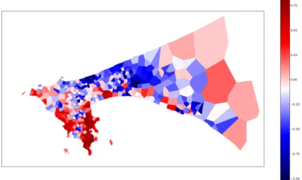
is organized on the scientific analysis of mobile phone datasets and the telecommunications company Orange organizes a "Data for devel-opment" (D4D) challenge, with the release of different mobile phone datasets with the purpose to contribute to societal development [62]. An example of what we can do using these data is shown in Fig. 3.

Figure 3: Relative difference of antenna mass between nigh and day in Dakar. Each Voronoi cell is colored with respect to the value

Mday(i)−Mnight(i)

Mday

In the report of the D4D Senegal challenge [63] we compute the mass of each antenna i during the day Mdayand during the night Mnight defines as the activity of the antenna i (i.e. the total number of calls and text messages sent and received from antenna i) during the day and night respectively, renormalized by the daily and nightly activity of the entire city. This quantity gives an idea of the changes in the spatial location of population over time.

An important issue concerning these new datasets is the accuracy of the information we extract from them. This is still not always well understood [58] and in a previous phase new methodologies to ex-tract data should be compared with the more traditional ones. This for example has been done by the authors in [64] who investigated this issue for the origin-destination matrix comparing the results ob-tained with twitter, cell phone data and surveys finding a good agree-ment.

4

M O D E L I N G A N D D I F F E R E N T A P P R O A C H E S

George Box claimed [65] "Essentially, all models are wrong, but some are useful". Helbing [66] added "Several models are right". It is more-over interesting to note that a model can have different interpreta-tions. This has been discussed several times by Thisse in [31] and Hel-bing in [67]. An example is the multinomial logit model [68,69] that can be derived in a utility-maximizing framework assuming rational individuals, but it can be also related to distributions of statistical physics and be compatible with a framework where individuals act without a strategy [70].

I am really tempted and interested in starting a philosophical dis-cussion about modeling but it would go far beyond the goal of this thesis. I refer the interested reader to the introduction of the Helbing book [66] that is focused on the modeling of social systems.

In this section, I will quickly summarize the modeling approaches used in economics, geography and computer science and then I will focus on the physicist’s one.

In the paradigm of complexity, geographers and computer scientists began to widely use and develop agent-based models. These consist in really complex numerical simulations that grasp as many details as possible. These kind of models however are often characterized by over-fitting and fine-tuning problems.

"With four parameters I can fit an elephant and with five I can make it wiggle his trunk" (Attributed to von Neumann by Enrico Fermi, as quoted

by [71]).

The big number of parameters and variables taken into account in these models, make it difficult to specify their inter-dependencies , to understand which of the parameters and mechanisms introduced are relevant for the phenomenon studied and which can be neglected. In order to understand the phenomenon is essential to identify the vari-ables and interactions that play a crucial role.

On the other side, most of economics model are very simplified and abstract, based on very strong assumptions such as the rational choice and the general equilibrium (see section1.1). This strict methodology

can be questioned [72].

The equilibrium assumption for example: the city is an out-of-equilibrium system [73] characterised by different time and space scales over which the variables evolve. The Equilibrium hypothesis can be done depending on the particular question asked after a discussion on the spatial and temporal scale that are involved (see [74] for a wider dis-cussion on this).

Concerning instead the rationality of individuals, Paul Ormerod ar-gues [75]:

"In many social and economic contexts, self-awareness of agents is of little consequence... No matter how advanced the cognitive abilities

of agents in abstract intellectual terms, it is as if they operate with relatively low cognitive ability within the system... The more useful

’null model’ in social science agent modeling is one close to zero intelligent. It is only when this fails that more advances cognition of

agent should be considered. "

However, beyond these particular and strict assumptions, writing complicated equations that are essentially impossible to solve does not contribute much to our understanding. Indeed hypothesis and approximations are necessary in order to obtain quantitative and em-pirically testable predictions. Economic models are thus interesting to get an insight on the different urban processes and on the possible socio-economic variables needed when studying urban systems, such as the spatial structure of rent and income, the job choice process, the impact of amenities and transportation. Nevertheless, these model have often a big drawback that is the lack of the relation between models and empirical evidences [72] as also the economist Krugman highlights at the end of its review [19]. The scientific validity of these models is thus questionable.

Empirical analysis is fundamental to understand urban systems behaviors, but is also not enough. Data can indeed be misleading without a theoretical framework for interpreting them (see for ex-ample [45, 76]) and understanding which are the interactions and processes underpinning the observations is important to inform and help urban policies makers. We thus need models, and empirical ob-servations to put constraints on them and help to identify universal regularities. Both data and models and the feedback loop between them are necessary in order to make progresses.

For a physicist the purpose of a model is to explain empirical observa-tions and to predict. But what does it mean to explain? to predict? to understand? As we discussed talking about the revolution in physics, physicists began to learn and they keep learning to change the mean-ing of the word prediction and the way to tackle problems dependmean-ing on the studied system, its typical scales and its characteristics. Some-times if we want to solve a problem we are just obliged to view it from another point of view.

"Models may be compared with city maps. It is clear that maps simplify facts, otherwise they would be quite confusing. We do not want to see any

single detail (e.g. each tree) in them. Rather we expect a map to show the facts we are interested in, and depending on the respective purpose, there are

quite different maps (showing streets, points of interest, topography, supply networks, industrial production, mining of natural resources, etc.)." [66]

Our aim is not to construct a mathematical model that reflect the full complexity of social interactions. We try instead to ask simple questions about urban systems and to propose simple models using ideas and tools from statistical physics, quantitative geography and spatial economics. These models will be characterized by the mini-mum number of variables needed to reproduce a certain effect, phe-nomenon or system behavior and they will give mathematical rela-tions that can be tested against data. The important and difficult issue is to identify the main ingredients and mechanisms involved in the particular phenomenon studied.

We do not want to describe all the details of the system, we aim in-stead to reach a better understanding of the so-called "stylized facts" and universal properties that we observe in data and that go beyond the details characterizing each city.

Roughly speaking we can summarize the physical approach through the following steps [77]

1. Ask simple questions 2. Look at data

3. Make a guess about the dominant mechanisms and build a min-imal model

4. Compute the consequences the model implies 5. Compare with data

and if there is not agreement with data, the model is wrong and you have to make another guess. In applying this methodology to urban systems, our choice of the ingredients and mechanisms to introduce in the model will be guided by geography and economic studies.

5

A B O U T T H I S T H E S I S

Given the huge variety of problems related to cities, it is impossible to discuss all aspects of cities at once.

The manuscript is organized in two parts. The first partiifocuses on the physical structure of the city that is investigated at two dif-ferent spatial resolutions: at the scale of the building lot in the first section6, and at a more coarse-grained scale in the second section7.

In the first section we tackle the phenomenon of urbanization begin-ning with an empirical analysis of geolocalized historical data, at the spatial scale of the building. This allow to monitor the urbanization process in time and at a very good spatial resolution.

In particular, we discuss how the number of buildings evolves with population and we show on different datasets that this "fundamen-tal diagram" evolves in a possibly universal way with three distinct phases. Once the universal pattern has been determined, we propose a stochastic model based on simple mechanisms to contribute to the understanding of the empirical observations. These results bring evi-dences for the possibility of constructing a minimal model that could serve as a tool for understanding quantitatively urbanization and the future evolution of cities.

In the second section we propose a continuous description of urban sprawl at a coarse-grained level with respect to the spatial unit of the building lots analysed in the first section.

If we begin by looking at data we observe that cities are characterized by a large number of different behaviors and do not display a simple unique pattern.

We then propose a slightly different approach focused on the study of a dispersion model that has been used extensively in the investigation of dispersions of animals in theoretical ecology, and also as a simpli-fied model for the growth of cancerous tumours. This model repre-sents a good candidate to describe the growth of an urban area based on a double process, the growth of surface area and the absorption of neighbouring towns. We are interested in understanding and explor-ing the different behaviors the model can produce and this can help us to get a better insight on the variety of behaviors observed in em-pirical data, that can be reinterpret and analyzed in light of the new acquired knowledge. In the second part of the thesis we introduce in our study socio-economic aspects. Indeed, we focus on commuting patterns and its relation to income. Once again we start from data, and we study the commmuting patterns of Denmark, US and Eng-land highlighting some regularities we observe. In a second step, we

consider the important economic job search model, the McCall model [78] that is based on an optimal strategy. We study the implications of the McCall model for the spatial distribution of distances between residences and jobs depending on the income and we show that they are not supported by empirical evidences. In a last part we propose a model based on the closest opportunity that meets the expectation of each individual that is able to predict correctly the behavior of the average commuting distance with income in terms of the density of jobs offers. More importantly, this model is able to correctly predict the form of the commuting distance distribution, its broad tail, and the data collapse predicted by its form. More generally, we propose here an alternative framework to study human or animal behavior, in which actions are taken not on the basis of an optimal strategy but on the first opportunity that is good enough. This framework would po-tentially find some applications in our understanding of foraging for example and other applications in ecology or finance where optimal control might be an incorrect assumption.

Part II

T H E P H Y S I C A L S T R U C T U R E O F C I T I E S

This part focuses on the physical structure of the city with the aim to get a better quantitative insight in the process of urbanization and its consequences. In section6we ana-lyze urban changes looking at the evolution in time of two urban indicators: the population and the number of build-ings. In section 7 instead, we use a coarse-grained scale with the aim to study one of the consequences of the ur-banization process that is the urban sprawl. We present a dispersal model as a candidate for describing the growth of an urban area based on a double process, the growth of surface area and the absorption of neighboring towns.

6

A F U N D A M E N TA L D I A G R A M O F U R B A N I Z AT I O N

6.1 i n t r o d u c t i o n

Understanding urbanization and the evolution of urban system is a long-standing problem tackled by geographers, historians, and economists and has been abundantly discussed in the literature but still repre-sents a widely debated problem (see [5]).

6.1.1 What do we mean by urbanization?

The first question we should ask when we aim to get a better insight into the urbanization process is "what do we mean by urbanization"? A well defined subject is an essential step to get a better understand-ing of it. The term urbanization has been indeed used in the literature with various definitions, and depending on the particular choice it can been considered as a continuous or an intermittent process [5].

Most of the time urbanization is measured by the fraction of indi-viduals living in urban areas. With this definition, urbanization rep-resents a continuous process that gradually increased in many coun-tries with a quick growth since the middle of the 19th century un-til reaching values around 80% in most european countries, [79]. In Fig. 4 we show this trend for more and less developed regions and

for the entire world. Although this characterization is widely used, it does not allow to get a deep understanding of the urban changes occurring in cities. Does the fraction of people living in urban ar-eas incrar-eases because fixed and stable defined urban systems become denser or does it increases because rural areas become urban and thus the number of urban centers increases or even because of urban sprawl?

Another definition has been introduced by [75] in its empirical anal-ysis of french cities and presented by [80] as a a theory of differen-tial urbanization in which urban changes are analysed looking at the changes in the population distribution in a system of cities character-ized by different sizes. The theory assumes that in general we observe the three regimes of urbanization, polarization reversal and counter-urbanization, and that are characterized by a net migration which favors the primate, intermediate, and small-sized cities, respectively (see Fig. 5). It thus describes a process of population redistribution

down the urban hierarchy, in which the term urbanization is associ-ated to the regime where the growth of the primate city is the faster one.

Figure 4: Percentage of urban population. Data from [6].

Figure 5: The figure represents the phases of urban development of a system of cities, according to the theory of differetial urbanization. Figure adapted from [80].

Yet another approach in the study of urban changes is presented in the stages of urban development proposed by [81], (see Fig.6) where the

phases of development are analyzed for a single urban agglomeration distinguishing the behavior of its inner part, the ’core’ from the one of the surrounding area, the ‘ring’.

According to this model, the city has a life cycle going from an early growing phase to an older phase of stability or decline, and four

main intermediate phases of development are identified. The first one called urbanization consists of a concentration of the population in the city core by migration of the people from outer rings. The second phase of suburbanization is characterized by a population growth of the urban agglomeration as a whole but with a population loss of the inner city and an increase in urban rings. During the third phase of (counterurbanization or disurbanization) the urban population decreases both in the core and the ring. Finally, the last phase of reurbanization displays a re-increase of the urban population. Within this framework, we observe that for most post-second war western countries urbaniza-tion was dominating in the 1950s followed by a suburbanizaurbaniza-tion in the 1960s during which the population moved from the city core to the suburbs. The standard theory of suburbanization suggests that this is driven by a combination of technological progress (leading to trans-port infrastructure development) and rising incomes [4, 79, 82]. In the 1970s we observe in many urbanized areas a regime of counter-urbanization where the population decreases. The significance of this regime and of the re-urbanization period for the 1980s and beyond, and more generally the possibility of a cyclic development are contro-versial topics (see for example [5]).

Figure 6: The figure represents the stages of urban development. Figure adapted from [79].

6.1.1.1 Data and definitions issues

In the previous section we discussed urban changes and the differ-ent meanings attributed to the word urbanization. It can concern the study of aggregate quantities as in the first definition, or a system of cities hierarchically organized in the second one, or a single urban agglomeration, analysing the relation between the core and its sur-rounding rings. When from a qualitative discussion we move to the

empirical analysis to better understand the phenomenon and test the-ories, we have to face the following questions: how do we establish what is urban and what is rural? Spatially, how do we determine the boundaries of the urban system? What is its core? And what its ring? Long time ago this task was easier, the urban center was enclosed by walls and beyond it was the countryside. From the 18th _{century on,} gradually, city walls began to be broken down and the urban agglom-erations started to spread out, the surrounding countryside began to be affected by an ’urbanization process’ as well. Establishing the de-limitation between urban and rural became a challenging task and the difficulty mainly arise from the fact that the concept of urban from which city boundaries are determined, is an abstraction that involves different factors, such as population density, labour supply and de-mand, and administration [83].

There are different definitions of cities depending on the historical period and on the country considered, which makes it difficult to conduct comparative and historical studies. Cities were defined in terms of population densities, or in terms of administrative bound-aries which tell nothing about urban sprawl. A more recent approach, is to study cities in terms of functional boundaries as the MSAs in US, the FUAs for the OECD and the LUZs in Europe, in which ur-ban center are defined according to a population density threshold ρ∗ and are connected to other areas for which the commuting flow to the urban center is higher than a threshold τ∗. However, these functional definitions are not consistent with each other. Recently, a non-ambiguous way to measure the extent of human agglomerations have been proposed. It is based on clustering techniques and called City Clustering Algorithm (CCA) [84, 85]. We remark moreover that all these definitions depend on the choice of threshold parameters. A variant has been proposed in [86], where different definitions and different choices of the thresholds are discussed, analyzing how they modify power-law behaviors observed in data.

6.1.2 Quantitative understanding

Even though urban development and the spatial distribution of resi-dences in urban areas are long-standing problems and were indeed discussed in many fields such as geography, history and economics; few of these approaches tackled this problem from a quantitative point of view ([28, 87–94]). Anas [95] presented an economic model for the dynamics of urban residential growth where different zones of a region exchange goods, capital, etc. according to some optimiza-tion rule. In the same framework the authors of [96] proposed a dy-namical central place model highlighting the importance of both de-terminism and fluctuations in the evolution of urban systems. For a review on different approaches, one can consult [97], where different

studies of population dynamics modeling are presented. In particu-lar, the author discusses the ecological approach, where ideas from mathematical ecology models are introduced for modeling urban sys-tems. The work in [98] is such an example. In it, the authors show how the phase portraits of differential equations can bring qualita-tive insights on urban systems behaviors. Other important theoretical approaches comprise the classical Alonso-Muth-Mills model ([82]) de-veloped in urban economics, and also numerical simulations based on cellular automata ([99]). More recently, the fractal nature of city structures (see the review [100]) served as a guide for the develop-ment of models ([94, 101, 102]). In particular, in [102], the authors proposed a variant of percolation models for describing the evolution of the morphological structure of urban areas. This coarse-grained ap-proach however neglects all economical ingredients and suggests that an intermediate way between these purely morphological approaches and economical models should be found.

For most of these quantitative studies however, numerical models usually require a large number of parameters that makes it difficult to test their validity and to identify the main mechanisms governing the urbanization process. On the other hand, theoretical approaches propose in general a large set of coupled equations that are diffi-cult to handle and amenable to quantitative predictions that can be tested against data. In addition, even if a qualitative understanding is brought by these theoretical models, empirical tests are often lacking.

6.1.3 New data

The recent availability of geolocalized, historical data (such as in [46] for example) from world cities [103], has the potential to change our quantitative understanding of urban areas and allows us to revisit with a fresh eye long-standing problems. Many cities created open-data websites [104] and the city of New York (US) played an impor-tant role with the release of the PLUTO dataset (short for Property Land Use Tax lot Output), where tax lot records contain very useful information about the urbanization process. For example, in addi-tion to the locaaddi-tion, property value, square footage etc, this dataset gives access to the construction date for each building. This type of geolocalized data at a very small spatial scale allows to monitor the urbanization process in time and at a very good spatial resolution.

These datasets allow in particular to produce ‘age maps’ where the construction date of buildings is displayed on a map (see Fig-ure7for the example of the Bronx borough in New York City). Many

age building maps are now available: Chicago [47], New York City US) [48], Ljubljana (Slovenia) [49], Reykjavik (Iceland) [50], etc. In addition to be visually attractive (see for example [105, 106]), these maps together with new mapping tools (such as the urban layers

1790 1846 1902 1958 2014

Figure 7: Map of buildings construction date for the case of the Bronx (New York City, US). Most of the buildings were constructed during the beginning of the 20th century, followed by the construction in some localized areas of buildings in the second half of the 20th century. (See section 6.2.1for details on the dataset).

proposed in [106]) provide qualitative insights into the history of spe-cific buildings and also into the evolution of entire neighborhoods. [107] studied the evolution of the city of Portland (Oregon, US) from 1851and observed that only 942 buildings are still left from the end of the 19th _{century, while 75, 434 buildings were built at the end of} the 20th century and are still standing, followed by a steady decline of new buildings construction since 2005. Inspired by Palmer’s map, [108] constructed a map of building ages in his home town of Ljubl-jana, Slovenia, and proposed a video showing the growth of this city from 1500 until now ([109]). Plahuta observed that the number of new buildings constructed each year displays huge spikes that sig-nalled important events: an important spike occurred when people were able to rebuild a few years after a major earthquake hit the area in 1899, and other periods of rebuilding occurred after the two world wars. In the case of Los Angeles (USA), the ‘Built:LA project’ shows the ages of almost every building in the city and allows to reveal the city growth over time ([110]).

Thanks to these new datasets, it is possible to monitor urban pro-cesses at a very small spatial resolution. In particular, we will focus on a given district or zone, without considering for the moment their position and their role in the whole urban agglomeration they belong to. We will ask quantitative questions about the evolution over time of the population and of the number of buildings, in order to under-stand if different districts of different cities can be compared with

each other. Surprisingly enough, such a dual information is difficult to find and – up to our knowledge – was not thoroughly studied at the quantitative level (except at a morphological level with fractal studies, [100]).

In this chapter we will show that the number of buildings versus the population follows the same unique pattern for all the cities stud-ied here. Despite the small number of cities analyzed, the strong sim-ilarities observed suggest the possibility of a universal behavior that can be tested quantitatively. In order to go further in our understand-ing of this unique pattern, we then propose a theoretical model and empirical evidences supporting it.

6.2 d ata a na ly s i s

We investigate the urban growth of four different cities: Chicago (US), London (UK), New York (US), and Paris (France). The urbanization process can be described by many different aspects and we will con-centrate on two main indicators. First, we consider the evolution of the population of urban areas and second, the evolution of the num-ber of buildings. These aspects concern both an individual-related aspect (the population) and an important physical aspect of cities, the buildings. Analyzing how the number of buildings varies with the population, we will try to understand the relation between these two elements.

In most datasets, we essentially have access to buildings that were built and survived until now. In this respect we do not take into account the destruction, replacement or modifications of buildings. Although replacement or modifications do not alter our discussion, replacement with buildings of another land-use certainly has an im-pact on the evolution of the population and could potentially lead to a major impact on the evolution of cities. As we will see in our model this can be in a way encoded in the ‘conversion’ process where a residential building is converted into a non-residential one. The im-portant point is to describe the temporal evolution of buildings and their function, and we encode all these aspects in the simpler quantity that is the number of buildings. Further studies are however certainly needed in order to clarify the impact of these points on our results. Finally, before proceeding to the description of the data and the em-pirical results, we want to remark that although these cities are among the most urbanized ones, they are characterized by quite different his-torical paths, with US cities being usually ’younger’ compared to the European ones. Chicago for example is a young city founded at the beginning of the 19th _{century, and Paris instead has an history of} about two thousands years.

6.2.1 Data description

Data will be studied at the spatial scale of the district and we will discuss this choice in the next section. This means that an important limitation that guided us for choosing these cities is the simultaneous availability of building age and historical data for district population. In particular, this second kind of data is difficult to find, mainly due to the change in time of administrative borders. In the following we describe the datasets, the historical range they cover and the way we exploited it.

6.2.1.1 Chicago data

We used the Building Footprints dataset (deprecated August 2015) provided by the Data portal of the City of Chicago [111]. For each building we have the information on the built year, the position and the geometrical shape from which we compute the building surface. By using the shapefiles of the 77 Chicago communities [112], we can deduce the community (and thus the side) where the building is lo-cated in. For each side we compute the average building surface al by averaging the building lot area over all the buildings with known built year, situated in the side. For Chicago the percentage of build-ings with known built year is 54%. Population data from each com-munity area come from [113] and they cover the period from 1930 to 2010.

6.2.1.2 London data

We used the dataset ‘Dwelling Age Group Counts (LSOA)’ [114], which contain the residential dwelling ages, grouped into approxi-mately 10-year age bins from pre-1900 to 2015 (the bin 1940 − 1944 is missing). The number of properties is given for each LSOA area and each age bin. From these data we deduce the number of buildings for each London district as function of the year. Data for the historical population of the London boroughs were obtained from ‘A Vision of Britain through time’ [115]. Finally we used OSOpenMapLocal [116] containing the geometrical shape of London buildings to compute the average footprint surface for each district. We note that in this last dataset some buildings are aggregated and rendered as homo-geneized zones. For this reason we computed the average building surface of each district by averaging over all the buildings belonging to the district having a footprint surface smaller than 700m2_{. In} or-der to locate the district to which a building belongs to, we used the shapefile of London districts boundaries [117].

6.2.1.3 New York data

We used data from the Primary Land Use Tax Lot Output (PLUTO) data file, developed by the New York City Department of City Plan-ning’s Information Technology Division (ITD)/Database and Appli-cation Development Section [118]. It contains extensive land use and geographic data at the tax lot level. PLUTO data files contain three ba-sic types of data: tax lot characteristics, building characteristics and geographic/political/administrative districts. In particular for each building of the city we are interested in the building’s borough, the building age and the surface of the lot. For each borough we compute the average building surface al (assumed to be given by the average building lot surface) over all the buildings in the borough and with known age (for New York city we have this information for 94% of

buildings). New York data cover the period from 1790 to 2013. For the historical population data, we used different sources [119–122] 6.2.1.4 Paris data

We used the dataset ‘Emprise Batie Paris’ provided by the open data initiative of the ‘Atelier Parisien d’urbanisme (APUR)’ [123]. For each building we have the information on the geometrical shape, from which we compute the building surface, the year built and the ar-rondissement the building is situated in. For each arar-rondissement we compute the average building surface alaveraging this quantity over all the buildings with known built year (i.e. the 57% of the buildings), situated in the arrondissement. Population data comes from [124] and since the actual arrondissements where defined in 1859, population data at the level of the arrondissements covers the period from 1861 to 2011.

6.2.2 Choice of the areal unit

An important discussion concerns the choice of the scale at which we study the urbanization process. This is related to the Modifiable Areal Unit Problem (MAUP) introduced by Oppenshaw [125] to high-light that the results of an empirical spatial analysis depend on the space zoning used (district, city, region, country). However, as ar-gued in [22] this is not necessary an issue, indeed different results at different scales can be considered as a source of knowledge on the studied phenomenon. Moreover, as discussed in the introduction (see section2.2.1), depending on the question asked there will be a more

appropriate spatial scale to choose. Here, we aim to analyse urban changes at a spatial scale that is large enough in order to obtain sta-tistical regularities, but not too large as different zones may evolve differently. Indeed geographers observed that the population density is not homogeneous and decreases in general with the distance to the center ([126, 127]). Also, most cities during their evolution tend to spread out, with the density decreasing in central districts and in-creasing in the outer ones ([128]); for this reason in the literature the core of the city is often analyzed in relation to its suburbs. In this study we aim to simplify the analysis and we focus on a fixed area without considering its role in the whole urban agglomeration; nev-ertheless we would like this area to be mostly homogeneous and not mixing zones behaving in different ways.

We choose to focus here on the evolution of administrative dis-tricts of each city. At this level, data is available and we can hope to exclude longer term processes. We will show in the following that districts in the different cities considered here, display homogeneous growth. More precisely, we consider the 5 boroughs of New York, the 9 sides of Chicago, the 20 arrondissements of Paris and the 33

don districts. Also, in this way we do not have to tackle the difficult problem of city definition and its impact on various measures (see section6.1.1.1) and focus on the urban changes of a given zone with

fixed surface area.

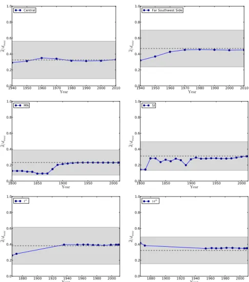
The cities studied here display very different scales, ranging from Paris with 20 districts for 2 − 3 millions inhabitants and an average of 5km2 per district, to New York City with 5 boroughs of very diverse area (from 60km2 _{for Manhattan to 183km}2 _{and 283km}2 _for Brook-lyn and Queens, respectively). The most important assumption that we will use here is that the development in each of these districts is relatively homogeneous. We test this assumption on Chicago, New York City and Paris for which we have the exact localization of new buildings (which we don’t have for London). For each district and at each point in time we compute the average distance d (normalized by the maximum distance in the district dmax) between new buildings in this district. We also compute the same quantity for a ‘null’ model for which the new buildings are distributed uniformly. The results are shown (Fig8) for a selection of districts of the different cities. In

this figure, we observe that despite the very diverse sizes of these dis-tricts, in all cities studied here, the development of new buildings is consistent with a uniform distribution, within these districts. This is a rather unexpected result as for example in Paris we have relatively ho-mogeneous districts while in New York City, the boroughs are much larger and aggregate together a variety of urban spaces. These results therefore show that despite the variety of cases, this choice of aerial unit provides a reasonable partition of space where the growth is homogeneous. In particular, it implies that a smaller area is not nec-essarily a good choice for studying the evolution of the number of buildings as it would suffer from strong sampling effects.

6.2.3 Population density growth

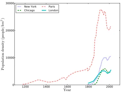
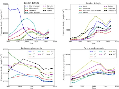
In order to provide an historical context, we first measure the evolu-tion of the populaevolu-tion density and then analyse the evoluevolu-tion of the number of buildings in a given district as a function of its population. In Fig. 9 we show the average population density for the four cities

studied here. This plot reveals that these different cities follow similar dynamics, at least at a coarse-grained level. After a positive growth and a population increase that accelerates around 1900, we observe a density peak. After this peak, the density decreases (even sharply in the case of NYC) or stays roughly constant. This decreasing regime is associated to the post World War years, defined by geographers as the suburbanization/counter-urbanization period. In the last years, New York City, Paris and London display a re-densification period. The possibility of this latter period has been proposed in some cyclic model as the stages of urban development one (see section 6.1.1).

Nev-1940 1950 1960 1970 1980 1990 2000 2010 Year 0.0 0.2 0.4 0.6 0.8 1.0 d/ dmax Central 1940 1950 1960 1970 1980 1990 2000 2010 Year 0.0 0.2 0.4 0.6 0.8 1.0 d/ dmax

Far Southwest Side

1800 1850 1900 1950 2000 Year 0.0 0.2 0.4 0.6 0.8 1.0 d/ dmax MN 1800 1850 1900 1950 2000 Year 0.0 0.2 0.4 0.6 0.8 1.0 d/ dmax SI 1880 1900 1920 1940 1960 1980 2000 Year 0.0 0.2 0.4 0.6 0.8 1.0 d/ dmax 1st 1880 1900 1920 1940 1960 1980 2000 Year 0.0 0.2 0.4 0.6 0.8 1.0 d/ dmax 14th

Figure 8: Homogeneity of growth in districts. Average distance between buildings at a given time (this distance is normalized by the max-imum distance found for each district). Top: Chicago (centrral and far southwest sides). Middle: New York City (Manhattan and Staten Islands). Bottom: Paris (1st and 14th arrondissements). The dotted line represents the average value computed for a random uniform distribution and the grey zone the dispersion computed with this null model.