HAL Id: hal-00968974
https://hal.inria.fr/hal-00968974
Submitted on 1 Apr 2014
HAL is a multi-disciplinary open access
archive for the deposit and dissemination of
sci-entific research documents, whether they are
pub-lished or not. The documents may come from
teaching and research institutions in France or
abroad, or from public or private research centers.
L’archive ouverte pluridisciplinaire HAL, est
destinée au dépôt et à la diffusion de documents
scientifiques de niveau recherche, publiés ou non,
émanant des établissements d’enseignement et de
recherche français ou étrangers, des laboratoires
publics ou privés.
Non-asymptotic state estimation for a class of linear
time-varying systems with unknown inputs
Da-Yan Liu, Taous-Meriem Laleg-Kirati, Wilfrid Perruquetti, Olivier Gibaru
To cite this version:
Da-Yan Liu, Taous-Meriem Laleg-Kirati, Wilfrid Perruquetti, Olivier Gibaru. Non-asymptotic state
estimation for a class of linear time-varying systems with unknown inputs. the 19th World Congress
of the International Federation of Automatic Control 2014, Aug 2014, Cape Town, South Africa.
�hal-00968974�
Non-asymptotic state estimation for a class
of linear time-varying systems with
unknown inputs
D.Y. Liu∗,∗∗ T.M. Laleg-Kirati∗W. Perruquetti∗∗∗,† O. Gibaru∗∗∗∗,†
∗CEMSE Division, King Abdullah University of Science and
Technology (KAUST), 23955-6900, Thuwal, Saudi Arabia (e-mail: [email protected] , [email protected])
∗∗INSA Centre Val de Loire, Universit´e d’Orl´eans, PRISME EA 4229,
Bourges Cedex 18020, France
∗∗∗LAGIS (CNRS, UMR 8219), ´Ecole Centrale de Lille, 59650,
Villeneuve d’Ascq, France (e-mail: [email protected])
∗∗∗∗LSIS (CNRS, UMR 7296), Arts et M´etiers ParisTech Centre de
Lille, 59046 Lille Cedex, France (e-mail: [email protected])
†Equipe Projet Non-A, INRIA Lille-Nord Europe, France´
Abstract:In this paper, we extend the modulating functions method to estimate the state and the unknown input of a linear time-varying system defined by a linear differential equation. We first estimate the unknown input by taking a truncated Jacobi orthogonal series expansion with unknown coefficients which can be estimated by the modulating functions method. Then, we estimate the state by using extended modulating functions and the estimated input. Both input and state estimators are given by exact integral formulae involving modulating functions and the noisy output. Hence, estimations at different instants can be non-asymptotically obtained using a sliding window of finite length. Numerical results are given to show the accuracy and the robustness of the proposed estimators against corrupting noises.
Keywords: Non-asymptotic estimation; Modulating functions method; State estimation; Linear time-varying systems; Unknown input.
1. INTRODUCTION
State estimation for linear systems is an important re-search topic in automatic control, and of great interest for engineers. In fact, for cost and technological reasons, the state can not be always measured. Therefore, state estimators, such as state observers, are often needed. Ob-servers usually converge asymptotically, which may not be useful in some applications. In this paper, we provide non-asymptotic and robust state estimators for a class of linear time-varying systems defined by a linear differential equation with an unknown input. Moreover, we provide also estimators for the input.
Among the methods that have been proposed recently for non-asymptotic state estimation is the algebraic method proposed by Fliess and Sira-Ramirez originally for linear identification [1]. The latter has been also extended to many applications, such as parameter estimation for noisy signals (see, e.g., [2, 3, 4, 5, 6]), and numerical differenti-ation (see, e.g., [7, 8, 9, 10, 11]). The main idea of this method is to apply some algebraic operations (such as differentiation and multiplication) to a linear differential equation of the analyzed signals in the Laplace opera-tional domain. When returning into the time domain, we can obtain a sequence of integral equations of the analyzed signals multiplied by some weight functions of
the Jacobi orthogonal polynomial. Then, estimators are given by integral formulae. Thus, estimations at different instants can be obtained using a sliding window of finite length. Consequently, this method is algebraic and non-asymptotic. Moreover, it exhibits good robustness prop-erties with respect to corrupting noises (see [12] for more theoretical details). When this algebraic method is used for numerical differentiation problem, thanks to the proposed integral formulae, it also refers to the differentiation by integration method well known for the Lanczos general-ized derivative (see [13] p. 324). The obtained algebraic differentiators have been used to design algebraic non-asymptotic observers for linear and non-linear systems (see, e.g., [14, 15, 17, 18, 19]). In the linear case [14, 15, 16], the proposed differentiators were obtained via the differ-ential equations which define the linear systems. Hence, they can be considered as model-based differentiators. The state variables have been accurately estimated without any time-delay. In the non-linear case [17, 18, 19], the used dif-ferentiators were obtained via the equations of truncated Taylor or Jacobi orthogonal series expansions of the output (see [7, 8, 9] for more details). Hence, these differentiators can be considered as model-free differentiators. Good state estimations have been obtained, but with a known time-delay produced by the truncated term error. Very recently,
model-free differentiators have been extended to estimate fractional order derivatives [20, 21].
Modulating functions method was introduced by Shinbrot in [22]. This method has been widely used for linear and non-linear identification of continuous-time systems (see, e.g., [23, 24]). Recently, the modulating functions method has been extended to parameter estimation of noisy sinu-soidal signals [25, 4]. However, to the best of our knowl-edge, it has not been extended to numerical differentiation problem. Rather than working in the Laplace operational domain as the algebraic estimation method, the basic idea of the modulating functions method is to transform the linear differential equation of the analyzed signals into a sequence of integral equations of these signals multiplied by the derivatives of different modulating functions via applying integration by parts in the time domain. Con-sequently, the modulating functions method has similar advantages to the algebraic estimation method. Moreover, it can be considered as a generalization of the algebraic estimation method in some cases (see, e.g., [4]). Indeed, the weight function of the Jacobi orthogonal polynomial is a modulating function. However, when tackling a complex problem, such as identification of fractional order systems, we can first be inspired by the algebraic estimation method by working in the operational domain (see, e.g., [26, 27]). Having these ideas in mind, inspired by [14, 15], we are going to extend the modulating functions method to design model-based differentiators so as to estimate the state for a class of linear time-varying systems. Moreover, inspired by the idea of designing algebraic model-free differentiators in [7, 8], we are going to also estimate the unknown input using the modulating functions method. Let us note that to the best knowledge of the authors, the estimations both of the state and the unknown input for a linear time-varying system have never been done neither by the algebraic method nor by the classical modulating function method.
This paper is organized as follows. In Section 2, we begin with the problem formulation, then we recall the generalized integration by parts formula and the properties of the Jacobi orthogonal polynomial. In Section 3, we first give a general definition for the modulating functions. Then, we use the modulating functions method to estimate the unknown input and the state. Numerical results are given in Section 4. Finally, we give some conclusions and perspectives in Section 5.
2. PRELIMINARY
2.1 Problem formulation
Let us consider a class of linear time-varying systems which can be defined by the following linear differential equation:
∀ t ∈ I,
M
∑
i=0
ai(t) y(i)(t) = u(t), (1)
where I = [0, T ] ⊂ R+, y is the output which is sufficiently
smooth enough, and u ∈ C(I) is the input which is assumed to be unknown. Moreover, we assume that ai,
for i = 0, · · · , M ∈ N, is piecewise i-times continuously differentiable on I, and is known. Let yϖ be a noisy
observation of y on I:
∀ t ∈ I, yϖ(t) = y(t) + ϖ(t), (2)
where ϖ is an integrable noise. In this paper, we want to estimate the unknown input and the state of the system defined by (1). For this purpose, we give some useful tools in the following subsection.
2.2 Jacobi orthogonal polynomials
The generalized integration by parts is a crucial tool for the use of modulating functions method. We recall this result in the following lemma which can be obtained by recursively applying the classical integration by parts method.
Lemma 1. Let f ∈ Cl(R) and g ∈ Cm(R), where l, m ∈ N∗
with m ≤ l. Then, for any interval [a, b] ⊂ R, we have: ∫ b a g(t) f(l)(t) dt = (−1)m ∫ b a g(m)(t) f(l−m)(t) dt + m−1 ∑ k=0 (−1)k[g(k)(t)f(l−1−k)(t)] t=b t=a. (3)
The nth (n ∈ N) order shifted Jacobi orthogonal
polyno-mial defined on [0, 1] is given as follows (see [29] p. 775):
Pn(α,β)(t) = n ∑ j=0 (n + α j )(n + β n− j ) (t − 1)n−jtj, (4)
where α, β ∈] − 1, +∞[. Let f and g be two functions belonging to C([0, 1]), then the scalar product ⟨·, ·⟩α,β of these functions is defined by (see [29] p. 774):
⟨f (·), g(·)⟩α,β = ∫ 1
0
wα,β(t) f (t) g(t) dt, (5)
where wα,β(t) = (1 − t)αtβ is the associated weight
function. Thus, by denoting its associated norm by ∥·∥α,β,
we obtain: ∥P(α,β) n ∥2α,β = Γ(α + n + 1) Γ(β + n + 1) Γ(α + β + n + 1) Γ(n + 1) (2n + α + β + 1). (6) where Γ(·) is the classical Gamma function (see [29] p. 255).
Finally, let us recall that if f ∈ C([a, b]) with [a, b] ⊂ R and h = b − a, then f can be expressed by the following Jacobi orthogonal series on [a, b]: ∀ t ∈ [0, 1],
f(a + ht) = +∞ ∑ i=0 ⟨ Pi(α,β)(·), f (a + h·)⟩ α,β ∥Pi(α,β)∥2α,β Pi(α,β)(t). (7) 3. MAIN RESULTS
3.1 Extended modulating functions
We extend the classical modulating functions by the fol-lowing definition.
Definition 1. Let [a, b] ⊂ R, l, k ∈ N with k ≤ l, and g be a function satisfying the following properties:
(P1) : g ∈ Cl+1([a, b]);
(P2) : g(i)(a) = 0, for i = 0, 1, . . . , l;
(P3) : g(i)(b) = 0, for i = 0, 1, . . . , k,
Then, g is called (l, k)th order modulating function on
[a, b]. If g satisfies only the properties (P1) and (P2) for
any k ∈ N, then g is called (l, −1)th order modulating
function on [a, b]. If l = k, then g is the classical lthorder
modulating function on [a, b] (see, [28]).
According to the previous definition, we can obtain that if α, β ∈ R∗
+, then the weight function wα,β of the shifted
Jacobi polynomials is a (⌊α⌋, ⌊β⌋)th order modulating
function on [0, 1], where ⌊α⌋ (resp. ⌊β⌋) refers to the largest integer smaller than α (resp. β).
3.2 Estimation of unknown input
The model-free differentiators were proposed in [7, 8, 9] by taking a truncated Jacobi series expansion which locally estimates the analyzed signal on a small sliding window. In this subsection, we estimate the unknown input in a similar way, where the coefficients in the truncated Jacobi series expansion are unknown. Then, these unknown coefficients can be estimated using the modulating functions method. Based on this idea, the following proposition is given. Proposition 1. Let yϖbe a noisy observation of the output
y of the linear time-varying system defined by (1), and {fn}Wn=0 be a set of (M − 1)thorder modulating functions
on [0, 1]. Then, an estimate of the unknown input u in (1) can be given by: ∀ t ∈ [h, T ] with h ∈]0, T ],
∀ τ ∈ [0, 1], ue(t + (τ − 1)h) = N ∑ i=0 ˜ λt,iP (α,β) i (τ ), (8)
where N, W ∈ N with N ≤ W , Pi(α,β)(·) is given by (4) with α, β ∈] − 1, +∞[, and ˜λt,i, for i = 0, · · · , N , is the
solution of the following linear system:
Af ˜ λt,0 .. . ˜ λt,N = Byϖ, (9) with Af(n + 1, i + 1) = ∫01fn(τ ) Pi(α,β)(τ ) dτ , and Byϖ(n + 1) = M ∑ i=0 (−1)i hi ∫ 1 0 Ft,h,i,n(i) (τ ) yϖ(t + (τ − 1)h) dτ , Ft,h,i,n(τ ) = fn(τ ) ai(t + (τ − 1)h), for n = 0, · · · , W and
i= 0, · · · , N .
Remark 1. Since ai is piecewise i-times continuously
dif-ferentiable on I, for i = 0, · · · , M , if there is a discontinuity on the sliding integration window [t−h, t], then the deriva-tives of Ft,h,i,n should be understood in the distribution
sense [30]. Proof.
Step 1. Using a truncated Jacobi series expansion: For any t ∈ [h, T ], by taking the following change of variable t → (t − h) + hτ in (1), we get: ∀ τ ∈ [0, 1], u(t + (τ − 1)h) = M ∑ i=0 ai(t + (τ − 1)h) y(i)(t + (τ − 1)h). (10)
Then, we take an Nth order truncated Jacobi series
expansion of u on [t − h, t]: ∀ τ ∈ [0, 1], uN(t + (τ − 1)h) := N ∑ i=0 λt,iPi(α,β)(τ ), (11) where λt,i= ⟨ Pi(α,β)(·),u(t+(·−1)h)⟩ α,β ∥Pi(α,β)∥2 α,β . Let us take uN as an
estimation of u, then (10) becomes:
N ∑ i=0 ˜ λt,iP (α,β) i (τ ) = M ∑ i=0 ai(t + (τ − 1)h) y(i)(t + (τ − 1)h), (12) where ˜λt,i are the estimation of the unknown coefficients
λt,i.
Step 2. Estimation of the unknown coefficients λt,i:
Let {fn}Wn=0 be a set of (M − 1)th order modulating
functions on [0, 1]. Then, by multiplying both sides of (12) by fn and integrating from 0 to 1, we get: for n =
0, · · · , W , ∀ t ∈ [h, T ], N ∑ i=0 ˜ λt,i ∫ 1 0 fn(τ ) P (α,β) i (τ ) dτ = M ∑ i=0 ∫ 1 0 fn(τ ) ai(t + (τ − 1)h) y(i)(t + (τ − 1)h) dτ. (13)
Then, by applying the generalized integration by parts formula given in Lemma 1, we obtain: for n = 0, · · · , W , ∀ t ∈ [h, T ], N ∑ i=0 ˜ λt,i ∫ 1 0 fn(τ ) Pi(α,β)(τ ) dτ = M ∑ i=0 (−1)i hi ∫ 1 0
Ft,h,i,n(i) (τ ) y(t + (τ − 1)h) dτ, (14)
where Ft,h,i,n(τ ) = fn(τ ) ai(t + (τ − 1)h). Let us mention
that all the boundary derivative values are eliminated by the properties (P2) and (P3) of fn. Consequently, the
coefficients, ˜λt,i, for i = 0, · · · , N , can be calculated by
solving the following linear system:
Af ˜ λt,0 .. . ˜ λt,N = By, (15) where Af(n + 1, i + 1) =∫ 1 0 fn(τ ) P (α,β) i (τ ) dτ , and By(n + 1) = M ∑ i=0 (−1)i hi ∫ 1 0
Ft,h,i,n(i) (τ ) y(t + (τ − 1)h) dτ , for n = 0, · · · , W and i = 0, · · · , N . Finally, this proof can be completed by substituting y by yϖ in (15).
✷ Error analysis for the estimation ue given in Proposition
1 can be given thanks to previous studies. On one hand, according to (11), the estimation uecontains a truncated
term error (see [8, 9] for more theoretical analysis). On the other hand, according to (12), the truncated term error in (11) is a source of error for ˜λt,i. Moreover, ˜λt,i contain
also a noise error contribution due to the noise in Byϖ (see [9, 4] for similar theoretical analysis).
If we take a set of Jacobi orthogonal polynomials multi-plied by their weight function and divided by the associ-ated norms as the used modulating functions in Proposi-tion 1, then the matrix Af becomes the identity matrix.
Hence, the unknown coefficients can be directly given without solving the linear system (9). Thus, inspired by this idea, we can give the following corollary.
Corollary 2. Let yϖ be a noisy observation of the output
y of the linear time-varying system defined by (1), and for n= 0, · · · , N ,
∀ τ ∈ [0, 1], fn(τ ) = wα,β(τ )
Pn(α,β)(τ )
∥Pn(α,β)∥2α,β
(16)
with α, β ∈]M −1, +∞[. Then, an estimate of the unknown input u in (1) can be given by: ∀ t ∈ [h, T ],
∀ τ ∈ [0, 1], ue(t + (τ − 1)h) = N ∑ i=0 ˜ λt,iPi(α,β)(τ ), (17) where ˜λt,i = M ∑ i=0 (−1)i hi ∫ 1 0 Ft,h,i,n(i) (τ ) yϖ(t + (τ − 1)h) dτ with Ft,h,i,n(τ ) = fn(τ ) ai(t + (τ − 1)h).
Proof. Since wα,β(τ ) = (1 − τ )ατβ with α, β ∈]M −
1, +∞[, using the Leibniz formula we can verify that {fn}Wn=0is a set of (M −1)thorder modulating functions on
[0, 1]. Then, according to the orthogonality of the Jacobi polynomial, we can deduce from (9) that:
Af(n + 1, i + 1) =
∫ 1
0
fn(τ ) Pi(α,β)(τ ) dτ
={ 1, if n = i,0, else.
Consequently, this proof can be completed using (9). ✷ Another way to get Corollary 2 is to take the scalar prod-uct ⟨·, ·⟩α,β involving the Jacobi polynomial Pn(α,β)(·)
∥Pn(α,β)∥2α,β to both sides of (10), such that the coefficients λt,i can
be directly obtained. Then, after applying the generalized integration by parts, we substitute y by yϖin the integrals
involving y. Thus, the estimations of λt,iin Corollary 2 do
not contain the error due to the truncated term in (11) any more.
Finally, if we fix the value of τ in Proposition 1 and Corollary 2, we can get an estimated value of u on each sliding window [t − h, t]. Let us recall that when approximating a function by its truncated Jacobi series expansion on a sliding window, we usually have large truncated term errors near the two extremities of the sliding window (see, e.g., [20]). Consequently, according to [7, 8, 9], we can take the value of 1 − τ as the smallest root of PN+1(α,β)to reduce the truncated term error. However, this
choice of τ produces a time-delay. More details are given in the numerical simulations section.
3.3 State estimation
In this subsection, we are going to estimate the successive derivatives y(i), for i = 0, · · · , M − 1, using the estimated input u and the observation yϖ in a sliding integration
window. For this purpose, we apply the extended modu-lating functions method. Unlike the classical modumodu-lating functions method where all the boundaries conditions are eliminated by the properties of the modulating functions,
we keep the right side boundary conditions which contain the derivative values of the output.
Proposition 3. Let yϖbe a noisy observation of the output
yof the linear time-varying system defined by (1), and ue
be an estimation of the unknown input. Then, the succes-sive derivatives of y can be estimated using a recursucces-sive way as follows: ∀ t ∈ [h, T ], ye(t) = (−1)M−1 G(M −1)t,h,M,0(t) ∫ t t−h gt,h,0(τ ) ue(τ ) dτ + M ∑ i=0 (−1)M+i G(M −1)t,h,M,0(t) ∫ t t−h G(i)t,h,i,0(τ ) yϖ(τ ) dτ, (18) and for n = 1, · · · , M − 1, ye(n)(t) = (−1) (M −n−1) G(M −n−1)t,h,M,n (t) ∫ t t−h gt,h,0(τ ) ue(τ ) dτ + n−1 ∑ k=0 M ∑ i=M −n+k (−1)i−k+M −n−1 G(M −n−1)t,h,M,n (t) G (i−k−1) t,h,i,n (t) y (k) e (t) + M ∑ i=0 (−1)i+M −n G(M −n−1)t,h,M,n (t) ∫ t t−h G(i)t,h,i,0(τ ) yϖ(τ ) dτ, (19) where gt,h,n, for n = 0, · · · , M −1, is a (M −1, M −2−n)th
order modulating function on [t − h, t] with h ∈]0, T ], Gt,h,i,n(τ ) = gt,h,n(τ ) ai(τ ).
Proof.
Step 1. Application of integration by parts:
For any t ∈ [h, T ] with h ∈]0, T ], we take a sequence of functions gt,h,n∈ CM([t−h, t]), for n = 0, · · · , M −1. Then,
by multiplying both sides of (1) by gt,h,n and integrating
from t − h to t, we get: ∀ t ∈ [h, T ], ∫ t t−h gt,h,n(τ ) u(τ ) dτ = M ∑ i=0 ∫ t t−h gt,h,n(τ )ai(τ ) y(i)(τ ) dτ. (20)
Then, by applying the generalized integration by parts formula given in Lemma 1, we obtain: for i = 1, · · · , M , for n = 0, · · · , M − 1, ∀ t ∈ [h, T ], ∫ t t−h Gt,h,i,n(τ ) y(i)(τ ) dτ = (−1)i ∫ t t−h
G(i)t,h,i,n(τ ) y(τ ) dτ
+ i−1 ∑ k=0 (−1)k[G(k)t,h,i,n(τ ) y(i−1−k)(τ )] τ=t τ=t−h, (21) where Gt,h,i,n(τ ) = gt,h,n(τ ) ai(τ ).
Step 2. Elimination of the derivative values at t − h: Let us assume that gt,h,n, for n = 0, · · · , M − 1, satisfies
the property (P2) by taking a = t−h and l = M −1. Then,
we can deduce that Gt,h,i,nalso satisfies the property (P2)
with a = t−h and l = i−1. Hence, all the derivative values at τ = t − h in (21) are equal to 0. Thus, (21) becomes: for n = 0, · · · , M − 1, ∀ t ∈ [h, T ],
M ∑ i=0 ∫ t t−h Gt,h,i,n(τ ) y(i)(τ ) dτ = M ∑ i=0 (−1)i ∫ t t−h
G(i)t,h,i,n(τ ) y(τ ) dτ
+ M ∑ i=1 i−1 ∑ k=0 (−1)kG(k) t,h,i,n(t) y (i−1−k)(t). (22)
Then, all the derivative values at t in (22) can be given in the following matrix: D =
G(0)t,h,1,n(t) y(0)(t) · · · G(0)t,h,M,n(t) y(M −1)(t) 0 · · · −G(1)t,h,M,n(t) y(M −2)(t) .. . . .. ... 0 · · · (−1)M−1G(M −1)t,h,M,n(t) y(0)(t) .
Step 3. Estimation of the derivative values at τ = t: We are going to calculate the boundary derivative values in the matrix D from the last line to the first line using extended modulating functions. For this purpose, we assume that gn, for n = 0, · · · , M − 1, also satisfies the
property (P3) with b = t and k = M − 2 − n. Hence, gn
is a (M − 1, M − 2 − n)th order modulating function on
[t − h, t]. Moreover, we can deduce that G(k)t,h,i,n(t) = 0, for k= 0, · · · , min(M − 2 − n, i − 1). Hence, the sum in (22) becomes: M ∑ i=1 i−1 ∑ k=0 (−1)kG(k) t,h,i,n(t) y (i−1−k)(t) = M ∑ i=M −n i−1 ∑ k=M −n−1 (−1)kG(k)t,h,i,n(t) y(i−1−k)(t). (23)
By applying a change of index k → i − 1 − k in (23), we get: M ∑ i=M −n i−1 ∑ k=M −n−1 (−1)kG(k)t,h,i,n(t) y(i−1−k)(t) = M ∑ i=M −n i−M +n ∑ k=0
(−1)(i−1−k)G(i−1−k)t,h,i,n (t) y(k)(t). (24)
Then, by changing the order of the sums in (24), we get:
M ∑ i=M −n i−M +n ∑ k=0
(−1)(i−1−k)G(i−1−k)t,h,i,n (t) y(k)(t) =
n ∑ k=0 M ∑ i=M −n+k
(−1)(i−1−k)G(i−1−k)t,h,i,n (t) y(k)(t). (25)
Hence, using (25), (20) becomes: ∀ t ∈ [h, T ], ∫ t t−h gt,h,n(τ ) u(τ ) dτ = M ∑ i=0 (−1)i ∫ t t−h
G(i)t,h,i,n(τ ) y(τ ) dτ
+ n ∑ k=0 M ∑ i=M −n+k
(−1)i−k−1G(i−k−1)t,h,i,n (t) y(k)(t), (26)
for n = 0, · · · , M − 1. By taking n = 0 in (26) we get: ∀ t ∈ [h, T ], y(t) = (−1) M−1 G(M −1)t,h,M,0(t) ∫ t t−h gt,h,0(τ ) u(τ ) dτ + M ∑ i=0 (−1)M+i G(M −1)t,h,M,0(t) ∫ t t−h
G(i)t,h,i,0(τ ) y(τ ) dτ. (27)
Then, for any n ∈ {1, · · · , M − 1}, we get: ∀ t ∈ [h, T ],
y(n)(t) = (−1) (M −n−1) G(M −n−1)t,h,M,n (t) ∫ t t−h gt,h,0(τ ) u(τ ) dτ + n−1 ∑ k=0 M ∑ i=M −n+k (−1)i−k+M −n−1 G(M −n−1)t,h,M,n (t) G (i−k−1) t,h,i,n (t) y (k)(t) + M ∑ i=0 (−1)i+M −n G(M −n−1)t,h,M,n (t) ∫ t t−h
G(i)t,h,i,0(τ ) y(τ ) dτ.
(28)
Finally, this proof can be completed by substituting y by yϖ and u by u
e in (27) and (28). Thus, the derivatives
y(n), for n = 1, · · · , M − 1, can be estimated in a recursive
way with the estimates of y(k), for k = 0, · · · , n − 1.
✷ Finally, we can remark that except the estimation error in the estimation of u, the differentiators proposed in Proposition 3 contain only the noise error contribution (see [4] for similar theoretical analysis).
4. SIMULATION RESULTS
In order to illustrate the accuracy and robustness against corrupting noises of the proposed estimators, we present some numerical results in this section.
Let us consider the following simplified model of a DC motor system (electric part is neglected) [15]:
∀ t ∈ I, ˙x1 = x2(t), ˙x2 = − 1 a(t)x2(t) + k a(t)u(t), (29)
where x1 is the angular position of the rotor, x2 is the
angular velocity of the rotor, y ≡ x1 is the output and
u is the input. The parameter k is a strictly positive constant, and a is a time-varying strictly positive param-eter. According to (29), we can obtain the following linear differential equation:
∀ t ∈ I, a(t) k y(t) +¨
1
k˙y(t) = u(t). (30) From now on, we assume that yϖ(t
i) = y(ti) + δϖ(ti) is a
discrete noisy observation of the output on I = [0, 20], with ti= Tsi, for i = 0, · · · , m, where Ts= 20m = 10−4(m = 2×
105) is an equidistant sampling period. δϖ(t
i) is simulated
from a zero-mean white Gaussian iid sequence, where the variance δ2 is adjusted such that the signal-to-noise ratio
SNR = 10 log10 ( ∑ |yϖ(t i)|2 ∑ |δϖ(ti)|22 ) is equal to SNR= 25dB. Moreover, we assume that the initial conditions are such that x1(0) = 1 and x2(0) = 0, the input is a sinusoidal
function u(ti) = 12 sin(ti), the parameters k = 1 and
a(ti) = 2 cos(0.2π ti) + 3. We can see the output y and
its discrete noisy observation yϖin Figure 1.
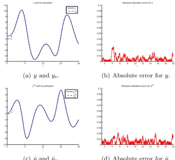
Firstly, we estimate y ≡ x1 and ˙y ≡ x2 using Proposition
3 in the case where we assume that the input u is known. In this example, we have M = 2. Hence, according to Proposition 3, we need two modulating functions of
0 5 10 15 20 −10 −5 0 5 10 15
Output and its observation
t
yϖ y
Fig. 1. The noise-free output and its noisy observation. (1, 0)th order and (1, −1)th order respectively. For this
purpose, we take gti,h,0(τ ) = (ti − τ )(τ − ti + h)
2 and
gti,h,1(τ ) = (τ − ti+ h)
2 where τ ∈ [t
i− h, ti] with ti≥ h
and h = 1.25. This kind of modulating functions that have a similar form to the weight function of the Jacobi polynomial have been already used in [4, 26]. Moreover, we apply the trapezoidal numerical integration method to approximate the integrals obtained in Proposition 3. We can see the obtained estimations and the associated absolute estimation errors in Figure 2.
Secondly, we estimate both the unknown input u and the state variables. On one hand, we use Corollary 2 to estimate u by taking h = 1.25, N = 1, and α = β = 3 such that fn is a 1st order modulating function on [0, 1],
for n = 0, 1, 2. Moreover, as shown in Subsection 3.2, we take 1 − τ = 0.3333 as the smallest root of P2(α,β) to reduce the truncated term error. Hence, this choice of τ produces a time-delay in the estimation of u. On the other hand, we take the same modulating functions as before and the obtained estimation of u in Proposition 3. Since the estimation of u contains a time-delay of value h(1 − τ ), it produces also a time-delay with the same value in the estimation of y and ˙y. We can see the obtained estimations, the shifted estimations and the associated absolute estimation errors in Figure 3.
5. CONCLUSIONS
In this paper, we have extended the classical modulating functions method to the numerical differentiation problem so as to estimate the states of a class of linear time-varying systems with unknown inputs. The design of the input and the state estimators has been inspired by the alge-braic free differentiators and the algealge-braic model-based differentiators respectively, without using a dynamic auxiliary system. Hence, these estimators have similar advantages to the recent algebraic estimation method. In-deed, they have been easily obtained without knowing the statistical properties of noises and have been exactly given by integral formulae leading to non-asymptotic properties and robustness against corrupting noises.
Different from the model-free differentiators obtained in [7, 8] using the noisy measurement of the signal to differ-entiate, the proposed input estimators were obtained via the differential equation defining the system. Moreover, unlike the model-based differentiator obtained in [15, 16] with complex mathematical deduction, the proposed state
0 5 10 15 20 −8 −6 −4 −2 0 2 4 6 8 10 12
y and its estimation
t y ye (a) y and ye. 2 4 6 8 10 12 14 16 18 20 0 0.01 0.02 0.03 0.04 0.05 0.06 0.07 0.08 0.09 0.1
Absolute estimation errors for y
t
(b) Absolute error for y.
0 5 10 15 20 −10 −8 −6 −4 −2 0 2 4 6 8
y(1) and its estimation
t
y(1)
ye (1)
(c) ˙y and ˙ye.
2 4 6 8 10 12 14 16 18 20 0 0.01 0.02 0.03 0.04 0.05 0.06 0.07 0.08 0.09 0.1
Absolute estimation errors for y(1)
t
(d) Absolute error for ˙y.
Fig. 2. State estimations where the input u is known.
0 5 10 15 20 −15 −10 −5 0 5 10 15
u and its estimation
t
u ue
shifted ue
(a) u, ue and shifted ue.
2 4 6 8 10 12 14 16 18 20 0
0.5 1 1.5
Shifted absolute estimation error for u
t
(b) Absolute error for shifted ue.
0 5 10 15 20 −8 −6 −4 −2 0 2 4 6 8 10 12
y and its estimation
t y ye shifted ye (c) y, yeand shifted ye. 2 4 6 8 10 12 14 16 18 20 0 0.01 0.02 0.03 0.04 0.05 0.06 0.07 0.08 0.09 0.1
Shifted absolute estimation errors for y
t
(d) Absolute error for shifted y.
0 5 10 15 20 −10 −8 −6 −4 −2 0 2 4 6 8 y(1)
and its estimation
t y(1) ye (1) shifted ye (1)
(e) ˙y, ˙yeand shifted ˙ye.
2 4 6 8 10 12 14 16 18 20 0 0.01 0.02 0.03 0.04 0.05 0.06 0.07 0.08 0.09 0.1
Shifted absolute estimation errors for y(1)
t
(f) Absolute error for shifted ˙y.
Fig. 3. State estimations where the input u is unknown. estimators are much easier to obtain and to understand thanks to the use of the generalized integration by parts formula and extended modulating functions.
Numerical results have been given in both cases where the input is known or not. In the first case, the state has been accurately estimated without time-delay. In the second case, a time-delay with a known value has been introduced to improve the estimation of the unknown input, which
has produced a time-delay with the same value in the estimations of the state. This time-delay was due to the truncated term error in the estimation of the input, and its value has been taken using the root of the first term in the truncated terms. In our future work, we are interested in the extension of the proposed method to state estimation for non-linear systems.
REFERENCES
[1] M. Fliess and H. Sira-Ram´ırez, An algebraic frame-work for linear identification, ESAIM Control Optim. Calc. Variat., vol. 9, pp. 151-168, 2003.
[2] D.Y. Liu, O. Gibaru, W. Perruquetti, M. Fliess and M. Mboup, An error analysis in the algebraic es-timation of a noisy sinusoidal signal, in Proc. 16th Mediterranean conference on Control and automation (MED’08), Ajaccio, France, 2008.
[3] M. Mboup, Parameter estimation for signals de-scribed by differential equations, Applicable Analysis, vol. 88, pp. 29-52, 2009.
[4] D.Y. Liu, O. Gibaru and W. Perruquetti, Parameters estimation of a noisy sinusoidal signal with time-varying amplitude, in Proc. 19th Mediterranean con-ference on Control and automation (MED’11), Corfu, Greece, 2011.
[5] W. Perruquetti, P. Fraisse, M. Mboup and R. Ushiro-bira, An algebraic approach for Humane posture esti-mation in the sagital plane using accelerometer noisy signal, in Proc. 51st IEEE Conference on Decision and Control, Hawaii, USA, 2012.
[6] R. Ushirobira, W. Perruquetti, M. Mboup and M. Fliess, Algebraic parameter estimation of a multi-sinusoidal waveform signal from noisy data, in Proc. 2013 European Control Conference, Zurich, Switzer-land, 2013.
[7] M. Mboup, C. Join and M. Fliess: A revised look at numerical differentiation with an application to non-linear feedback control, in Proc. 15th Mediterranean Conference on Control and Automation (MED’07), Athenes, Greece, 2007.
[8] M. Mboup, C. Join and M. Fliess, Numerical dif-ferentiation with annihilators in noisy environment, Numerical Algorithms, vol. 50, no. 4, pp. 439-467, 2009.
[9] D.Y. Liu, O. Gibaru and W. Perruquetti, Error anal-ysis of Jacobi derivative estimators for noisy signals, Numerical Algorithms, vol. 58, no. 1, pp. 53-83, 2011. [10] D.Y. Liu, O. Gibaru and W. Perruquetti, Differen-tiation by integration with Jacobi polynomials. J. Comput. Appl. Math., vol. 235, no. 9, pp. 3015-3032, 2011.
[11] L. Kiltz and J. Rudolph, Parametrization of alge-braic numerical differentiators to achieve desired filter characteristics, in Proc. 52nd IEEE Conference on Decision and Control, Florence, Italy. 2013.
[12] M. Fliess, Analyse non standard du bruit, C.R. Acad. Sci. Paris, Ser. I, vol. 342, pp. 797-802, 2006. [13] C. Lanczos, Applied Analysis, Prentice-Hall,
Engle-wood Cliffs, NJ, 1956.
[14] M. Fliess and H. Sira-Ram´ırez, Reconstructeurs d’´etats, C.R. Acad. Sci. Paris, S´erie I, vol. 338, pp. 91-96, 2004.
[15] Y. Tian, T. Floquet and W. Perruquetti, Fast state es-timation in linear time-varying systems: an algebraic approach, in Proc. 47th IEEE Conference on Decision and Control, Cancun Mexique, 2008.
[16] Y. Tian, T. Floquet and W. Perruquetti, Fast state estimation in linear time-invariant systems: an alge-braic approach, in 16th Mediterranean Conference on Control and Automation (MED’08), Ajaccio, Corsica, France, 2008.
[17] D.Y. Liu, O. Gibaru and W. Perruquetti: Error anal-ysis for a class of numerical differentiator: application to state observation, in Proc. 48th IEEE Conference on Decision and Control, Shanghai, China, 2009. [18] G. Zheng, L. Yu, D. Boutat and J.P. Barbot,
Alge-braic observer for a class of switched systems with Zeno phenomenon, in Proc. 48th IEEE Conference on Decision and Control, Shanghai, China, 2009. [19] F.J. Bejarano, W. Perruquetti, T. Floquet and G.
Zheng, State reconstruction of nonlinear differential-algebraic systems with unknown inputs, in Proc. 51st IEEE Conference on Decision and Control, Hawaii, United States, 2012.
[20] D.Y. Liu, O. Gibaru, W. Perruquetti and T.M. Laleg-Kirati, Fractional order differentiation by integration with Jacobi polynomials, in Proc. 51st IEEE Confer-ence on Decision and Control, Hawaii, USA, 2012. [21] D.Y. Liu, O. Gibaru and W. Perruquetti,
Non-asymptotic fractional order differentiators via an al-gebraic parametric method, in Proc. 1st International Conference on Systems and Computer Science, Vil-leneuve d’ascq, France, 2012.
[22] M. Shinbrot, On the analysis of linear and nonlinear dynamic systems from transient-response data, Na-tional Advisory Committee for Aeronautics NACA, Technical Note 3288, Washington, 1954.
[23] T.B. Co and S. Ungarala, Batch scheme recursive pa-rameter estimation of continuous-time system using the modulating functions method, Automatica, vol. 33, no. 6, pp. 1185-1191, 1997.
[24] H. Unbehauen and G.P. Rao, A review of identifi-cation in continous-time systems, Annual Reviews in Control, vol. 222, pp. 145-171, 1998.
[25] G. Fedele and L. Coluccio, A recursive scheme for frequency estimation using the modulating functions method, Appl. Math. Comput., vol. 216, pp. 1393-1400, 2010.
[26] D.Y. Liu, T.M. Laleg-Kirati, O. Gibaru and W. Perruquetti, Identification of fractional order sys-tems using modulating functions method, in Proc. 2013 American Control Conference, Washington, DC, USA, 2013.
[27] N. Gehring and J. Rudolph, An Algebraic Approach for Identification of Linear Systems with Fractional Derivatives, arXiv:1302.4071, 2013.
[28] H.A. Preising and D.W.T. Rippin, Theory and appli-cation of the modulating function method. I: Review and theory of the method and theory of the spline type modulating functions, Computers and Chemical Engineering, vol. 17, pp. 1-16, 1993.
[29] M. Abramowitz and I.A. Stegun, editeurs, Handbook of mathematical functions, GPO, 1965.
[30] L. Schwartz, Th´eorie des distributions, 2nd ed., Her-mann, 1966.