Performance of range-only TMA

HAL Id: hal-01820128

https://hal.archives-ouvertes.fr/hal-01820128

Submitted on 22 Jun 2018

HAL is a multi-disciplinary open access

archive for the deposit and dissemination of

sci-entific research documents, whether they are

pub-lished or not. The documents may come from

teaching and research institutions in France or

abroad, or from public or private research centers.

L’archive ouverte pluridisciplinaire HAL, est

destinée au dépôt et à la diffusion de documents

scientifiques de niveau recherche, publiés ou non,

émanant des établissements d’enseignement et de

recherche français ou étrangers, des laboratoires

publics ou privés.

Performance of range-only TMA

Annie-Claude Perez, Claude Jauffret, Denis Pillon

To cite this version:

Annie-Claude Perez, Claude Jauffret, Denis Pillon. Performance of range-only TMA. 2017 IEEE 7th

International Workshop on Computational Advances in Multi-Sensor Adaptive Processing (CAMSAP),

Dec 2017, Curacao, France. �10.1109/CAMSAP.2017.8313076�. �hal-01820128�

Performance of Range-Only TMA

Annie-Claude Pérez

#1

,

Claude Jauffret

#2

, Denis Pillon

*3

#

Aix Marseille Univ, Univ Toulon, CNRS, IM2NP, Marseille, France CS 60584, 83041 TOULON Cedex 9, France

1 _{annie-claude.perez@univ-tln.fr} 2 _{jauffret@univ-tln.fr}

* _Retired

Thonon France

3 _{pillon_denis@orange.fr}

Abstract—Range-only target motion analysis (ROTMA) is the

topic of this paper: we focus our study on the numerical aspect and performance of the maximum likelihood estimates (MLE) for some scenarios when the noise polluting the measurements is additive and Gaussian. The performance is compared to the Cramér–Rao lower bound (CRLB).

I. INTRODUCTION

Range-only target motion analysis (ROTMA) has been treated in the literature for various applications, the target having a constant velocity (CV) motion: for example in [1], [2] and [3], maritime surveillance radar systems, ISAR (inverse synthetic aperture radar), are studied. It offers also an efficient way to calibrate a sonar array [4]. ROTMA is encountered in the robotic domain by radio-frequency [5] [6]. Local observability was analysed by the rank of the Fisher information matrix (FIM) [7]. Global observability conditions were proposed recently in [8] and [9]. In the same vein, we present here some aspects of estimation (which was not addressed in [8] and [9]), in particular for scenarios where observability is not acquired and for which the FIM is full-ranked, or conversely for scenarios where the trajectory of the target is observable, but the FIM is singular. This motivates the structure of our paper.

In section II, we present the assumptions and notations. Section III is devoted to the special case where the observer is in CV motion too. In section IV, the observer’s trajectory is composed of two legs. Here, the target’s trajectory can be observable or not [8]. Section V presents a case where the order of the observer’s kinematic model is greater than that of the target, and still the trajectory of the target is unobservable [9]. We end with a more favourable case: the observer’s trajectory contains an arc of a circle and this suffices to guarantee observability [9]. The conclusion follows.

II. HYPOTHESES,DEFINITIONS AND NOTATIONS A. Model of Target’s and Observer’s Kinematics

A target (T) and an observer (O) move in the same plane, given a Cartesian system. The target has a CV motion all along the scenario, while the observer maneuvers (the term “maneuver” is employed when the observer is not in CV motion).

For the observer, the position and velocity at time t are respectively _P

 

_t O and

 

 

dt t dP t

V_O  O . Both are concatenated

into the vector X_O

 

t 



P_OT

 

t V_OT

 

t



T. For the target, the

notations are similar: PT

 

t ,

 

dt t dP V_T  T , and

 



_T

 

_T



T T T T t P t V X  . Obviously, P_T

 

t P_T

 

0 tV_T . Note that whatever t , XT

 

t entirely defines the target’s trajectory. For a chosen *t , the state vector XT

 

t* will be simply denoted X 



x y x y



T . The motion of the target relative to the observer is given by POT

 

t PT

 

t PO

 

t

and by

 

 

dt t dP t V OT

OT  . We define the vector

 

t X

 

t X

 

t

XOT  T  O . All the angles are clockwise-positive:

the angle



North,W



is denoted W. The range and the bearing at time

t

are given respectively by _r

 

_t  _POT

 

_t and

 

t POT

 

t

 .

B. Measurements Model and Estimate

For the sake of simplicity, the notations r and _k _k will stand for _r

 

_tk and 

 

_tk , respectively. In order to emphasize the functional link of _{r with the state vector X , we use the k} notation rk

 

X . The range measurement collected at



k



t

tk 1 and denoted rm,k obeys the equation

 

k

k k

m r X

r,   (1), where k is the measurement noise

assumed to be Gaussian, temporally white and zero mean; its standard deviation is _r,k . The set of N available range

measurements is





N m m m m r r r

r  _,1, _,2,, _, . The aim of the RO-TMA is to estimate the state vector X given the measurementsr . Note that in all the scenarios, the observer _m starts from PO

 

0 



0 0



T. The chosen estimate is the MLE

(or equivalently the LSE since the noise is additive and Gaussian). Its empirical covariance matrix will be compared to the Cramér–Rao lower bound (CRLB), which is the inverse of the FIM for unbiased estimators.

III. THE OBSERVER’S TRAJECTORY CONSISTS OF ONE LEG ONLY

In [8], we showed that when the observer is in CV motion, the trajectory of the target is observable up to an isometry (rotation or axial symmetry). We characterized the set of

targets (true target and ghost-targets)

O

in the same range as the target of interest:





 

 

                   

 I2 H 0 0 , H beingan orthogonal matrix

O O OT OT V P V P O .

O

can be defined by a 3-dimensional state vector

 

 

T      2 2 * 2 * T _{OT OT} OT OT t V P t V P

Z . Indeed, for any *t , we

have rk2 AkZ, with Ak



1 tkt*



tkt*



2



. Therefore, the range rk

 

X is reparametrized into rk

 

Z . This property

allows us to define a linear estimate. A. Linear Estimate

Let us consider the measurement equation (1) and express

the squares of its two elements: 2 , , 2 2 ,k k 2k rk rk m r r

r     . The noise intervening in this new

equation is then 2

, ,

2rk rk rk whose first two moments are



2



2

, ,

2

E r_k_rk_rk _r and Var



2r_k_r,k_r2_,k



2_r2



2r_k2_r2



(since

k r,



is Gaussian). We introduce then another “measurement”: 2

2 ,

,k mk r

m r 

   .We define also the “noise”:

2 2 , , 2_{k rk rk r} k r   

    whose first two moments are now

 

0 E_k  and

 





2 , 2 2 2 2 2

Vark  r rk r k. So, we end up

with the set of measurement equations

k k

k k

m r  Z 

 _,  2 A_k  _{for k1 , ,N . Note that}

k

 is zero-mean but no longer Gaussian. Still, it is legitimate to compute the weighted linear least squares estimator of Z that

minimizes the criterion

_{ }

_





   N k k m k Z Z C 1 2 , 2 , 1 k A  _ :                 





   N k k m k N k k WLS Z 1 , 2 , 1 1 2 , 1 1 ˆ _    T k k T kA A A

which is unbiased. Its covariance matrix is

 

1 1 ₂ 2 2 2 1 1 2 , 2 1 1 1 4 1 ˆ     _                     





N k k r k r N k k WLS r r Z Cov T _k k k T kA A A A   _ .

The computation of _ZˆWLS assumes the knowledge of 2

k

r . To alleviate this, in practice, we replace 2

k r by r_m2_,k:                 





   N k k m k m N k mk WLS Z 1 , 2 , , 1 1 2 , , 1 1 ˆ _    T k k T kA A A , with



2 2



, 2 2 , ,mk 2r 2rmk r    .

B. Efficiency of the Linear Estimate The FIM is given by

 

k T Z k Z N k r ROTMAZ 



 r  r 1 2 1  F with T k A k k Z r r 2 1   . Hence

_{ }

k T kA A F



  N k k r ROTMA r Z 1 2 2 1 4 1  and the CRLB is

 

_



 



1 Z Z ROTMA ROTMA F

B . The theoretical Cramér–Rao

inequality is respected: 1 1 2 2 2 2 1 1 2 2 2 1 1 1 4 1 4                           





N k k r k r N k k r r r r k T k k T kA A A A     , that is,

 

 

WLS ROTMAZ  CovZˆ B 1. When _k r_k r _{1 ,for any} 2 2   _{, then}

_{ }

_{ }

WLS ROTMA Z CovZˆ B .

The proposed estimator

WLS

Zˆ is hence approximately efficient. Numerous simulations (not reported here) have confirmed this conclusion.

IV. THE OBSERVER’S TRAJECTORY CONSISTS OF TWO LEG Now, the observer’s trajectory is composed of two legs, not necessarily traveled with the same speed: the velocities are _VO,1 when t and _VO,2 when t . The motion equation is _PO

 

_{t PO}

  

_{  t}



_VO,i . We know from Proposition 3 of [8] that one ghost at most exists whose

trajectory is defined by



_{ }







O O V V G X X X X O O     I2 S ,2 ,1 , where O

X stands for X_O

 

t* , and _{ }

1 , 2 , 2VO VO S is the matrix of

the symmetry around the line spanned by the vector 1 , 2 , O O V V  . To minimize

 



 

           N k Rk k k m r X r X C 1 2 , ,  , we have

recourse to the Gauss–Newton algorithm which will return Xˆ or X_G



_{V V }





X X_O



X_O O O       ˆ ˆ 1 , 2 , 2 S I , in unobservable

cases. Two scenarios have been considered: in the first one, the target’s trajectory is observable, and in the second one, proposed in [3], the target’s trajectory is unobservable. For each scenario, 500 Monte Carlo simulations have been run. For each simulation, we compute the MLE Xˆ and, if existing, the corresponding ghost Xˆ . The performance of the MLE is _G evaluated by its empirical bias and the comparison of the empirical standard deviations of its components with the square roots of the diagonal elements of the CRLB.

A. Observable Scenario

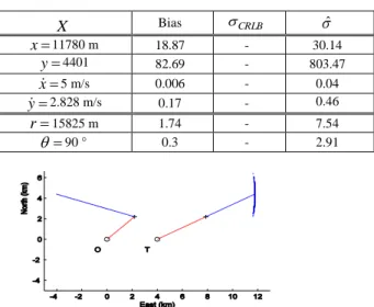
The first leg of the observer is characterized by a heading of 45° and a speed of 4 m/s. The instant of its heading change is 780s. During its second leg, the speed and the heading of the observer are equal to 8.49 m/s and –70.53°, respectively. The target starts at PT

 

0 



4,000 0



T(m), its

speed is 5.74 m/s, and its heading is 60.5°, corresponding to velocity VT 



5 2 2



T(m/s). The duration of the scenario is

1

Let Aand B be two symmetric matrices, A B means that the matrix BA is a non-negative matrix.

26 min. The measurements are acquired every 4 s (t4s), and the standard deviation of the noise is _r50 m. The

estimates and the performance are given at the final time. Fig. 1 depicts the scenario and the 500 estimates (O and T are for the initial positions of the observer and the target, respectively). Because the FIM is singular [8], the CRLB cannot be computed; therefore in Table I the column “CRLB”

contains no value. We observe that the sets of MLEs are “croissant-shaped”. This is why we present the results in Cartesian coordinates for the estimated target’s position





T

y

x and in polar coordinates



r 



Tfor the estimated relative position of the target w.r.t. the observer.

TABLEI

PERFORMANCE OF THE MLE AT FINAL TIME

X Bias CRLB ˆ  x 11780 m 18.87 - 30.14  y 4401 82.69 - 803.47  x 5 m/s 0.006 - 0.04  y 2.828 m/s 0.17 - 0.46  r 15825 m 1.74 - 7.54   90 ° 0.3 - 2.91

Fig. 1. The scenario and the estimates in an observable leg-by-leg case Numerous other simulations with various scenarios allow us to conclude that the MLE is unbiased. But we cannot claim that the MLE reaches the CRLB, because for such scenarios, the FIM is singular.

B. Unobservable Scenario(see [3])

In [3] the authors proposed the following scenario whose duration is 30 min to test a particle filter. The first heading and the speed of the observer are respectively -80° and 2.57 m/s. At t=15 min, it changes its course and the second heading is 146° and keeps the same speed. At the very beginning, the target is at P_T

 

0 



7,071 7,071



T(m), its

heading is -135° and its speed is 7.72 m/s (see Fig. 2(a)). The sampling rate is equal to 60 s and the standard deviation is

20



r

 m. As in [3], the estimates are given at time t*=26 min. In Table II, we give the estimate of the state vector at this time. Fig. 2(b) depicts the 90%-confidence ellipsoid (in red) together with the cloud of the position estimates (in blue), and their corresponding ghost-estimates (in red). Here, despite the presence of a ghost, the MLE is efficient. Note that adding a third leg does not guarantee observability [8].

TABLEII

PERFORMANCE OF THE MLE AT TIME t*=26 MIN.

X Bias CRLB ˆ  x -1444.8 m 6.84 10.93 11.12  y -1444.8 m 15.21 12.84 12.86  x -5.46 m/s 0.001 0.03 0.03  y -5.46 m/s 0.002 0.04 0.04  r 455.05 m 0.49 11.09 11.99   165.31 ° 0.11 1.60 1.64

Fig. 2. (a) The scenario and the estimates in Clark’s scenario [3], (b) magnification around the estimates.

V. THE OBSERVER IS IN CONSTANT ACCELERATION MOTION In the two scenarios presented hereafter, the initial velocity vector of the observer is



10 2



T(m/s). Its acceleration vector

is



0.0416 0



T (m/s2). In both scenarios, we choose

m

r 20

 and t1s.

A. Example of Observable Case

The target starts at



4000 0



T (m), with a velocity equal to





T

2

10 (m/s). Note that the observer and the target are on a rendezvous route. In this case the FIM is singular [9].

The estimates and the performance are given in Table III. TABLEIII

PERFORMANCE OF THE MLE AT FINAL TIME

X Bias _CRLB _ˆ  x -410 m 2.31 - 5.58  y 710 m 85.30 - 78.48  x 10 m/s 0.02 - 0.04  y 2 m/s 0.43 - 0.48  r 1319 m 2.80 - 3.13



 -90 ° 3.70 - 3.41

B. Example of Unobservable Case

The target starts at



2000 3464



T (m) with a velocity





T 3 . 16 6 .

14 (m/s). The observer and the target are not on a

rendezvous route and the bearings are not constant. Three ghosts exist (the maximum number of ghosts). Fig. 3 depicts the result: the estimates of the initial and final position of the target (T), and the couples of estimates of the three ghost-targets’ positions (G). Note that the three other solutions are computed from the MLE returned by the algorithm [9].

Fig. 3. The scenario and the estimates in an unobservable case. The estimate and its performance are given in Table IV.

TABLEIV

PERFORMANCE OF THE MLE AT FINAL TIME

X Bias _CRLB ˆ  x 7241.4 m 14.47 53.58 59.29  y 9315.7 m 10.22 37.19 41.84  x 14.6 m/s 0.02 0.39 0.39  y 16.3 m/s 0.03 0.21 0.21  r 10678 m 0.09 3.73 3.70   36 ° 0.1 0.35 0.39

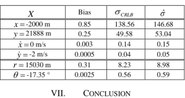
VI. THE OBSERVER’S TRAJECTORY CONTAINS AN ARC OF A CIRCLE

Now the observer’s trajectory is composed of two legs linked by an arc of a circle. The target’s trajectory was proved to be observable in [9]. No problem of convergence is indicated in our numerous simulations, provided the number of measurements during the arc of a circle is greater than 50 (otherwise, the routine can be stalled in a local minimum). In the scenario presented here, the initial position of the

observer is





T

000 , 10 1000

 (m) with speed equal to 4 m/s.

Its first heading is 90°. At time 1700s, it begins its circular maneuver and finishes it at time 2980s. At this time its new heading is equal to 225°. Meanwhile, the target has started at



_{2000 25,000}



T_{(m), with a speed equal to 2}

m/s following a route equal to 180°. The total duration of the scenario is 26 minutes. The standard deviation is 50 m. The

performance is summarized in Table V: we observe again that the MLE is efficient. Numerous simulations, not reported here, confirm this claim.

TABLEV

PERFORMANCE OF THE MLE AT FINAL TIME

X Bias CRLB ˆ  x -2000 m 0.85 138.56 146.68  y 21888 m 0.25 49.58 53.04  x 0 m/s 0.003 0.14 0.15  y -2 m/s 0.0005 0.04 0.05  r 15030 m 0.31 8.23 8.98   -17.35 ° 0.0025 0.56 0.59 VII. CONCLUSION

Three types of scenario were used to study the MLE in ROTMA: observable scenarios with nonsingular FIM, observable scenario with singular FIM and unobservable scenario with nonsingular FIM. For the first one, the MLE is efficient. For the second, the MLE is unbiased, but we cannot compute the CRLB. For the last, the MLE restricted to the local solution corresponding to the true target is efficient too. When several solutions exist (presence of ghost-targets), we are able to give the other solution(s) from the one returned by the algorithm. This study could be extended to the case of maneuvering targets as in [10].

REFERENCES

[1] Ristic, B., Arulampalam S. and McCarthy J., “Target Motion Analysis using Range-Only Measurements: Algorithms, Performance and Application to ISAR Data”, Signal Processing, Vol. 82, (2002), 273-296.

[2] Sathyan, T., Arulampalam, S. and Mallick, M., “Multiple Hypothesis Tracking with Multiframe Assignment Using Range and Range-rate Measurements”, In Proceedings of the International Conference on Information Fusion, Chicago, USA, July 2011.

[3] Clark, J.M.C, Kountouriotis, P.A, and Vinter, R.B., “A Gaussian mixture filter for Range-Only Tracking”, IEEE Transactions on Automatic Control, V. 56, N°3, (March 2011), 602 – 613.

[4] Pillon, D., “Method for Antenna Angular Calibration by Relative Distance Measuring”, Patent WO 2006/013136, 09.02.2006.

[5] Cevher, V., Velmurugan, R., and McClellan, J.H., “A range-only multiple target particle filter tracker”, In Proceedings of the International Conference on Acoustics, Speech and Signal Processing, Vol. 4, Toulouse, France, May 2006.

[6] Huang, G.P., Zhou, K.X., Trawny, N.T, and Roumeliotis S.I., “A Bank of Maximum A Posteriori Estimators for Single-Sensor Range-only Target Tracking”, In Proceedings of the American Control Conference, Marriott Waterfront, Baltimore, MD, USA, June 30-July 02, 2010. [7] Song, T.L., “Observability of Target Tracking with Range-Only

Measurements”, IEEE Journal of Oceanic Engineering, vol. 24, No. 3 (July 1999), 383-387.

[8] Pillon, D., Pérez-Pignol, A.C., and Jauffret, C., “Observability: Range-Only vs. Bearings-Range-Only Target Motion Analysis for a Leg by Leg Observer’s Trajectory”, IEEE Transactions on Aerospace and Electronic Systems, 52, 4 (Aug. 2016), 1667–1678.

[9] Jauffret, C., Pérez, A.C., and Pillon, D., “Observability: Range-Only vs. Bearings-Only Target Motion Analysis when the Observer Maneuvers Smoothly”, To appear in IEEE Transactions on Aerospace and Electronic Systems.

[10] Clavard, J., Pillon, D., Pignol, A.C. and Jauffret, C., “Target Analysis of a Source in a Constant Turn from a Nonmaneuvering Observer”, IEEE Transactions on Aerospace and Electronic Systems, AES-49, 3 (Jul. 2013), 1760-1780.