Modal analysis of an ultrafast frequency comb: From classical to quantum spectral correlations

HAL Id: tel-01261469

https://hal.archives-ouvertes.fr/tel-01261469

HAL is a multi-disciplinary open access archive for the deposit and dissemination of sci-entific research documents, whether they are pub-lished or not. The documents may come from teaching and research institutions in France or abroad, or from public or private research centers.

L’archive ouverte pluridisciplinaire HAL, est destinée au dépôt et à la diffusion de documents scientifiques de niveau recherche, publiés ou non, émanant des établissements d’enseignement et de recherche français ou étrangers, des laboratoires publics ou privés.

classical to quantum spectral correlations

Valérian Thiel

To cite this version:

Valérian Thiel. Modal analysis of an ultrafast frequency comb: From classical to quantum spectral correlations. Quantum Physics [quant-ph]. Universite Pierre et Marie Curie, 2015. English. �tel-01261469�

l'Université Pierre et Marie Curie

présentée par

Valérian THIEL

pour obtenir le grade de Docteur de l’Université Pierre et Marie Curie sur le sujet:

Analyse modale d’un peigne de fréquences femtoseconde :

Correlations spectrales classiques et quantiques

Modal analysis of an ultrafast frequency comb:

From classical to quantum spectral correlations

Soutenue le 19 Octobre 2015 à Paris

Membres du jury :

M. Marco BARBIERI Rapporteur

M. Yanne CHEMBO Membre du jury

M. Scott DIDDAMS Rapporteur

M. Claude FABRE Membre invité

M. Sébastien PAYAN Membre du jury

who has always put knowledge and education in front of everything

Contents

Acknowledgements viii

Introduction 1

I Measuring with ultra-fast frequency combs

5

1 The modes and states of a beam of light 6

1.1 The classical electromagnetic field. . . 7

1.1.1 Description of the real electromagnetic field . . . 7

1.1.2 Fourier space formalism . . . 8

1.2 Modal description. . . 9

1.2.1 Temporal and spectral modes . . . 9

1.2.2 Spatial modes . . . 10

1.2.3 Spatio-temporal modes. . . 12

1.2.4 Basis change . . . 13

1.2.5 Power and energy . . . 13

1.3 The quadratures of the classical field . . . 15

1.3.1 Quadrature amplitudes. . . 15

1.3.2 Quadrature fluctuations . . . 16

1.4 Quantization of the field. . . 17

1.4.1 Bosonic operators . . . 17

1.4.2 Modal decomposition. . . 17

1.4.3 Quadrature operators. . . 19

1.4.4 Relation to the classical field . . . 20

1.5 Quantum states . . . 21

1.5.1 Density operator . . . 21

1.5.2 Wigner function. . . 21

1.6 Gaussian states . . . 22

1.6.1 Definition and quantum covariance matrix . . . 22

1.6.2 Examples of Gaussian states . . . 23

2 Femtosecond ultrafast optics 27 2.1 Description of pulses of light . . . 28

2.1.1 Optical frequency combs. . . 28

2.1.2 Energy and peak power . . . 31

2.1.3 Moments of the field . . . 31

2.1.4 Gaussian pulses . . . 32

2.2 The influence of dispersion . . . 34

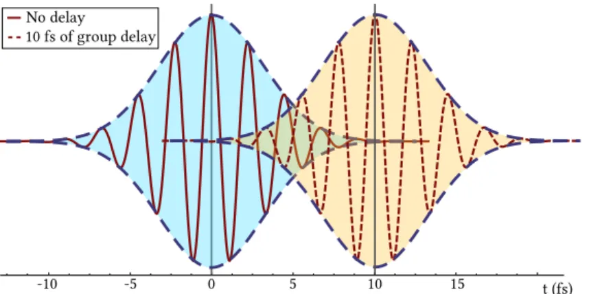
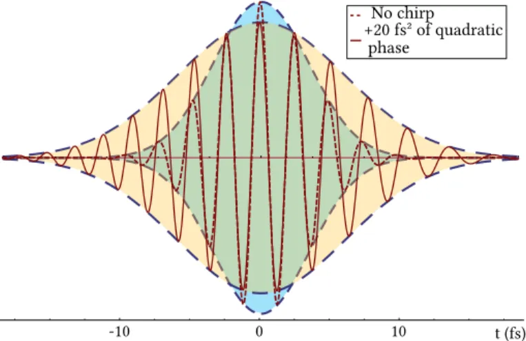
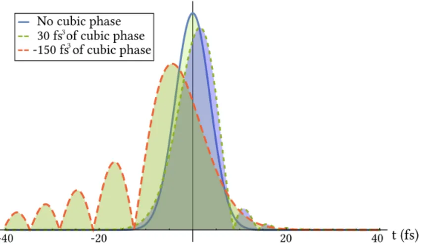
2.2.1 Spectral and temporal phases . . . 34

2.2.2 Effects on the pulse shape . . . 35

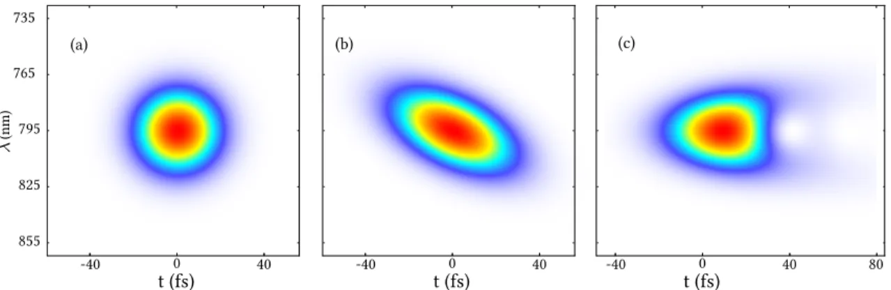
2.3 Representations of the pulse . . . 39

2.3.1 Time-frequency distributions . . . 39

2.3.2 Some examples . . . 41

2.3.3 Experimental realizations . . . 42

2.4 Generation of pulses of light . . . 42

2.4.1 Steady-state laser cavity . . . 43

2.4.2 Mode-locked lasers . . . 44

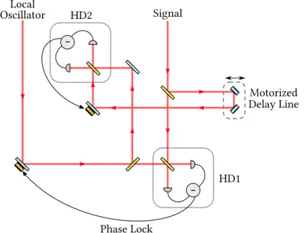
3 Revealing the multimode structure 49 3.1 General experimental scheme . . . 50

3.1.1 Laser source . . . 51

3.1.2 Interferometric photodetection . . . 52

3.1.3 Pulse shaping . . . 56

3.2 Signal measurement . . . 61

3.2.1 Modulations of the field . . . 61

3.2.2 Data acquisition . . . 63

3.3 Mode-dependent detection . . . 66

3.3.1 Quantum derivation . . . 66

3.3.2 Spectrally-resolved homodyne detection . . . 68

3.3.3 Temporally-resolved homodyne detection . . . 71

3.3.4 Addendum: single diode homodyne detection . . . 73

II Quantum metrology

75

4.1.1 Displacements of the field in specific modes . . . 77

4.1.2 Sensitivity . . . 79

4.1.3 The Cramér-Rao bound . . . 79

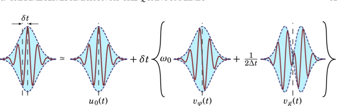
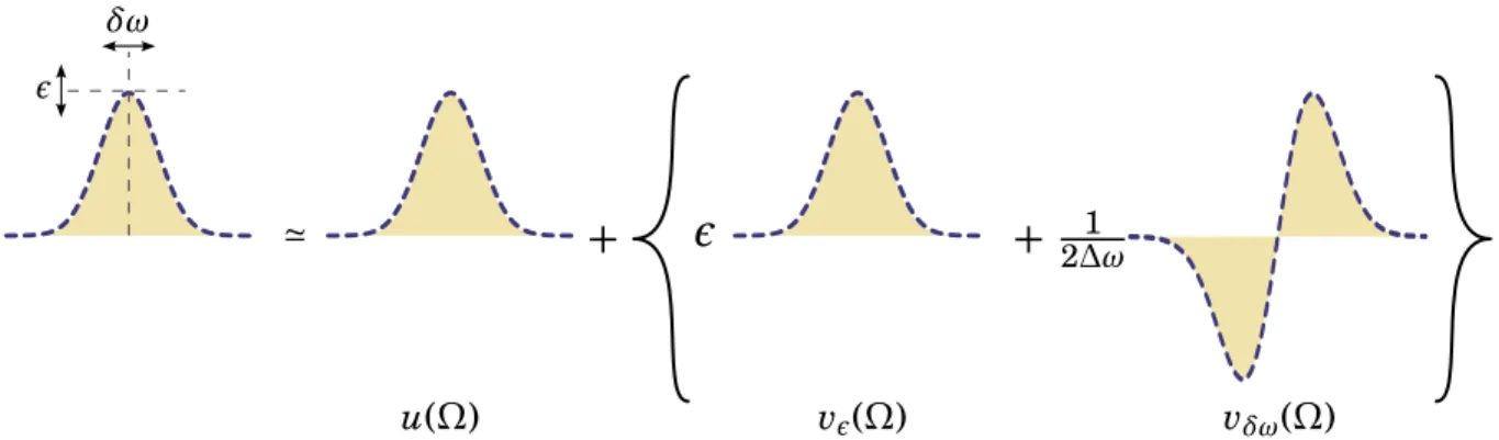
4.2 Spectral and temporal displacements . . . 80

4.2.1 Temporal displacements . . . 80

4.2.2 Spectral displacements . . . 82

4.2.3 Conjugated parameters . . . 85

4.3 Space-time coupling: a source of contamination . . . 92

4.3.1 Transverse displacements . . . 92

4.3.2 Homodyne contamination. . . 94

5 Measuring the multimode field 97 5.1 Experimental details . . . 98

5.1.1 Measurement strategy . . . 99

5.1.2 Phase modulation at high frequencies. . . 100

5.1.3 Spatial filtering . . . 103

5.2 Interferometer calibration . . . 104

5.2.1 Calibration of displacement . . . 106

5.2.2 Sensitivity measurement. . . 110

5.3 Multipixel detection . . . 111

5.3.1 Design and construction . . . 111

5.3.2 Gain calibration . . . 114

5.3.3 Space-wavelength mapping . . . 116

5.3.4 Clearance . . . 117

5.4 Spectrally-resolved multimode parameter estimation . . . 117

5.4.1 A glimpse at the multimode structure . . . 117

5.4.2 Signal extraction . . . 120

5.4.3 Heterodyne measurements: the need for a stable reference . . . 123

5.4.4 Space-time positioning . . . 124

5.4.5 Dispersion . . . 129

5.4.6 Quantum spectrometer. . . 132

III Noise analysis of an ultra-fast frequency comb

136

6.2.2 The cavity’s comb . . . 144

6.2.3 Simulations . . . 145

6.3 Experimental realization. . . 147

6.3.2 Design and construction . . . 147

6.3.3 Cavity lock . . . 148

6.3.4 Environnemental pressure dependency . . . 149

6.3.5 Noise properties . . . 151

7 Experimental study of correlations in spectral noise 153 7.1 The modal structure of noise . . . 154

7.1.1 Introduction and motivations . . . 154

7.1.2 The noise modes . . . 154

7.2 Measuring spectral correlations in the noise. . . 155

7.2.1 Classical covariance matrix . . . 155

7.2.2 Retrieving the fluctuations . . . 157

7.2.3 Experimental scheme . . . 158

7.3 Experimental results . . . 161

7.3.1 Amplitude and phase spectral noise . . . 161

7.3.2 The noise modes . . . 162

7.3.3 Collective parameters projection . . . 164

7.3.4 Phase-amplitude correlations . . . 165

7.3.5 Real-time laser dynamics analysis . . . 166

IV Going further with quantum frequency combs

169

8.1.1 Creation of squeezed states . . . 171

8.1.2 Parametric down conversion with an optical frequency comb . . . 172

8.1.3 Objectives and perspectives . . . 173

8.2 Single-pass squeezing . . . 174

8.2.1 Parametric down conversion . . . 174

8.2.2 Eigenmodes of the parametric down conversion . . . 175

8.2.3 Expected efficiency . . . 178

8.3 Second harmonic generation . . . 179

8.3.1 Efficiency . . . 179

8.3.2 The influence of temporal chirp . . . 182

8.4 An ultra-fast squeezer . . . 183

8.4.1 Pump generation . . . 183

8.4.2 Synchronously pumped optical parametric amplifier. . . 184

8.5 Perspectives . . . 185

8.5.1 Quantum enhanced metrology . . . 185

Conclusion and outlooks 189

Appendix A Medium dispersion 192

A.1 Sellmeyer equation . . . 192

A.2 Wave-vector dispersion . . . 192

A.3 Application to delay and dispersion estimation . . . 193

Appendix B Projective measurements by pulse shaping 195

B.1 Pulse shaping the time-of-flight mode . . . 196

B.2 Locking on the time-of-flight mode . . . 197

B.3 Dispersion measurement . . . 198

Appendix C Experimental construction of the detection modes 202

Appendix D Conjugated variable of space-time position 204

D.1 Detection mode for a global displacement . . . 204

D.2 Detection mode for a spectral displacement . . . 205

Acknowledgements

This dissertation is the conclusion of three years of work, work that could never have hap-pened without all the people that contributed to it. And in term of people that I had the privi-lege to work with, I believe it will prove hard in the future to replicate such a remarkable work environnement.

Before all, I would like to thank my jury, for reviewing my thesis on such short notice, and for bringing very interesting insight to the work. I can only imagine how daunting it must be to review such a long document, and you have my sincere gratitude for that.

In my opinion, what is probably the most important aspect of research in general is team work. Being part of a united group increases productivity and has the advantage of looking forward to going to work every day. Working in the quantum optics group of LKB was for me a perfect realization of this statement.

Therefore, I would like to thanks everybody in the LKB for being nice colleagues and co-workers, for sharing their different ways of working around a cup of coffee, or simply for discussing a broad variety of subjects among highly educated people. Moreover, the presence of people from all over the world allowed interesting insights into the world in general, making it suddenly a much smaller place, and making you feel more like a citizen of the world rather than of a single nation. Thanks also to the engineers and administrative people without who our work would be impossible. In particular, thanks to Thierry, Romain, Laetitia and Michel for flawlessly taking care of virtually every investment. A gigantic “thank you” to Monique, with-out who this place wouldn’t run as good as it is today. I wish all the best to her successor, Nora, who is already proving to be as exceptionally efficient at her job ! Another very sincere and loving acknowledgement to the electronics workshop, with Brigitte and Jean-Pierre, for their incredible work. The research that is presented in this thesis would most certainly have been very different without their knowledge and service. Walking into the electronics workshop for soldering work or just chatting was always a pleasure, and that is once again thanks to the people that work here. Thanks also to the IT department, Serge, Corinne, Jeremie and Mathilde for their great job at taking care of our computers and networks, globally making working in the lab easier. Thanks to Annick and Bintou, who were always nice and smiling every morn-ing, and for keeping my desk from collapsing under the weight of the mess I negligently made (sorry about that).

I would like to thank also the other research groups at the LKB and other labs. Notably, I am thankful to the optomechanics group of LKB in general for allowing me to start learning optics and quantum optics during my studies. Thanks in particular to Tristan for his teaching and counsel, thanks to Antoine for being always nice and cheerful, making today a very good director for the lab. My sincere thanks go to Alexandros, for introducing me to the work and

for giving a glimpse of what research should be. You taught me a lot of what I know today, and I am deeply grateful for that. Moreover, the intense pleasure that was procured by the process of cavity alignement will forever be etched in my mind. Thanks also to my friends from SYRTE, who showed me that metrology could-sometimes-be fun, with who my relationships were as fruitful as they were joyful and learning experiences, and for sharing a rather interesting conference in Prague.

A special thanks to our former interns, who allowed me to express my teaching personality (which I hope I did well) that I love showing. Thanks to Adrien and Martin for being so eager to learn, and for participating to the fun in the lab; Francesco, also for the fun he’s brought, for bringing more of that italian theoretician dimension to the team; Catx, for all the nice time we’ve shared and all the interesting discussion we’ve had, for bringing the sun with her every day (which I think you took away with you: bring it back !) and for being such a friendly, always smiling, very interesting person.

Finally and most importantly, there are all those colleagues that I today call friends, thanks to all the wonderful time we had outside of work. I wish to acknowledge from the bottom of my heart: all of my colleagues from my Master at ENS, Baptiste, Marion, Hugo, Thomas, Raphael, Rémi, Camille and so forth, for being such nice friends that made hard years of learning much more fun that I originally expected; Roman for sharing his last PhD year with me, walking me through the experiment, teaching me the delicate nature of metrology, the magic of crazy glue, and for, globally, giving me the German experience (what is regularly refereed to in the group as the Schmeissner®experience, something that no Man can forget); Renné, also for introducing me to the lab and the way things worked; Hanna, for not pushing charges against me; Pierre, for the same reason (although I know he would have enjoyed it) and for having spent some good time with us in Munich; Vanessa, for putting up with my appetite for German profanities and my unreasonable behavior in general; Valentin, for all the interesting discussion on theoretical physics with a russian accent we’ve had (but mostly for everything that wasn’t science related, such as the poster sessions at the DPG); Ale, for the amount of man-love that we still share today around beers, buratta, parmigiana and 80’s movies; Giulia, for being Giulia: words are not sufficient to describe how amazing this woman is♥; the same goes for Pu, for all the great time we shared together, all the cooking, dancing and singing♥; all the people from Cai Labs, J-F for being a great captain, for all the great time we’ve had sailing around the Greek islands, and Guillaume for the fun we’ve had in the lab. All of you people greatly contributed to making me a better person, and I will never forget all the time we’ve had together.

Another huge acknowledgement goes to the Unit, Clément and Jon, my brothers from other mothers, for having turned the lab into some kind of underground disco room, where the amount of hard work and productivity was always directly proportional to the fun we’ve had. It was always a genuine pleasure coming to work early in the morning and to go back home late at night. As hard as the work was, it was definitely worth it. So thanks from the bottom of my heart to Clément, without who I wouldn’t be here, for being such a great friend, for making life in the lab better, for bringing the spirit of party with him everyday, for throwing

amazing parties and dinners, for renting LED-blasters, for cooking Tiramisu, for buying italian salamee, for all the “Game over, man” situations, for sharing interesting rocket, airplane designs and delta-v optimization on Kerbal Space Program®, for his ability to make lemonade with a strong, single crushing gesture, for being my Linux Guru when I needed one, for his impressive mastery of the German side at Company of Heroes... Concerning Jon, words are also lacking to describe how incredibly lucky I was to accomplish my PhD with you. You taught me most of what I know about optics today, and I feel like I’ve learned more in these three years that I have during all my studies, and that is thanks to you. Your impressive knowledge of a broad variety of subject made working with you a precious experience, one I will also never forget. It is worth stressing that I believe that none of the work presented in this dissertation would have been possible without you, and it has truly been a privilege working with you. And again, the amount of work that we accomplished together is only matched by the amount of fun we’ve had together. It has been a lot of hard work, but it has also been a LOT of beers at the pub nextdoor, a lot of Lebanese sandwiches at 2AM, where I really enjoyed all the discussion that we’ve had about science, life and death. I shall never forget these days, I cherish the memory of California with you, Mission Peak (which was just a bit more challenging than expected), San Francisco, the rat parade, the Farmer’s Market... Thanks to both of you brothers, we’ve had the time of our lives during these years. In the name of the parameter estimation experiment, we would also like to thank Jameson, 1664, Chouffe, Leffe, Glenfiddich, the bathroom next to the lab, the people at Epsilon and Inevitable, the B-52 and madeleine shooters, black magic, voodoo magic, blood magic, Dante, my friend Jack, our mastah Vlad, El Scorpio, John Matrix, Bennett, Ash, Toni, Gunther, the Throne of Blood, the Centercom and its Tegam slave, the Warclub of Affliction, the Finger of Death, the Tooth of Sorrow, the Holy Horn, the Swing of Redemption and the Four Riders of the Apocalypse: the experiment would never have ended without them. Last, but not least, my most sincere thanks go to our bosses, Nicolas and Claude. Working under your direction has truly been a pleasure for multiple reasons. First, because you both are among the most brilliant person I had the chance to meet, such that learning from you has always been very rewarding. Then, because you have very kind personalities, and appreciate all the small things in life that make it worth living. I will always remember the pic-nics, group meeting / buffets, dinners and so on that we shared. It really helped make the group something unique, which created bonds not unlike a family. So thank you again, it has been a privilege working in the shadow of geniuses ! In term of latest addition to the team of brilliant people, Vale is there too, strengthening the italian, feminine presence in the group. Thanks you so much for your cheesecake (which should be put somewhere on your professional resume), and also for the short time we’ve spend together: you’re gonna do really fine in this group, and I foresee great things happening for you (which you definitely deserve).

All of this would also never have been possible without the support of my family. Thanks to my sisters and parents who supported me (quite literally at first) in my endeavor, who made me push always harder to reach the top. Also, I cannot be thankful enough to Tiphaine, whose love and attention allowed her to put up with my frequent mis-behavior, for taking so good

Introduction

The ability to perform precise measurements is a fundamental aspect of all quantitative science. To determine the value of a parameter in a physical system, an experimentalist uses a probe to interact with the system. By measuring the way the probe has been altered by its interaction with the system, it is possible to deduce the value of the parameter. Any probe can however be intrusive in the sense that it affects the physical system on its interaction, thus altering the response of the system to its presence. From a classical physics point of view, the usage of a beam of light as a probe is adapted to a non-intrusive measurement since it can be attenuated to a point where its interaction with matter is negligible.

For instance, light has been used extensively to the purpose of estimating distances. More than2000years ago, Eratosthenes estimated the circumference of the Earth using geometric consideration of the shadow cast by the Sun. If the same measurement were made today using current data, the retrieved value would be accurate to less than1%.

Accuracy is a fundamental concept in experimental science. It defines how different the value of a parameter will be when an experiment is repeated several times. The finite accuracy is a direct consequence of other physical phenomena that limit the knowledge of a variable, which may be described as the noise in a measurement. Without noise, any measurement would be always perfect.

The discovery in the end of the 18th century of the wave-like nature of light gave birth to the field of interferometry, allowing to measure distances with a precision limited only by the wavelength of light. In 1894, Michelson measured the length of a platinium-iridium standard by interferometry and defined it in terms of an emissive wavelength of cadmium. He advocated the use of wavelengths as a natural standard for distance [Michelson 94]. In 1960, the meter was redefined in terms of the emissive wavelength of krypton, replacing the platinium-iridium standard. Today, the meter is defined from the speed of light. Light became an even more widespread measurement tool since the advent of lasers, which brought a source of light that is highly coherent both spatially and temporally.

As a recent example, the usage of light as a tool to measure long distances with good accuracy has resulted in the estimation of the distance between the Earth and the Moon with an accuracy of a few millimeters [Murphy Jr 08]. This measurement was achieved by sending pulses of light on a retroreflector on the Moon and measuring their time of arrival. This measurement is called atime-of-flight measurement, which is less accurate than an interferometric measurement. The ability to distinguish between redundant information on distance, called ambiguity range, is on the order of the wavelength of light for an interferometric measurement, while it is on the order of the distance between subsequent pulses for a time-of-flight measurement. The latter then offer a better dynamics, since the spacing between pulses of light is much higher than

its wavelength. Combining interferometric and time-of-flight measurements then allows to merge high dynamics and sub-wavelength precision.

In order to combine the dynamics of the time-of-flight measurement performed with pulsed light and the precision obtained by interferometric measurement,optical frequency combs ap-peared as ideal tools for the task. A frequency comb consists of a large number of equally spaced optical frequencies with a narrow linewidth, and a fixed phase relationship between them. In the temporal domain, this corresponds to a train of short pulses emitted at equal in-tervals. The development of mode-locked lasers, and in particular Titanium-Sapphire lasers in the 1990' [Spence 91], resulted in the realization of such frequency comb with pulses as short as a few femtosecond. The realization of many stabilization techniques allows today to pro-duce very stable frequency combs, making them perfect tools for metrology and spectroscopy [Udem 02].

For the purpose of high precision measurement, the accuracy of an experiment accomplished using an optical frequency comb is limited mostly by the noise of the source. For a time-of-flight measurement, the accuracy is limited by the fluctuation of the repetition rate, calledtiming jit-ter, whereas an interferometric measurement is limited by the fluctuations in the each optical carrier, generally calledphase noise. The ability to characterize and measure these fluctuations is essential to their stabilization [Paschotta 05].

These fluctuations can be described as arising from technical sources, such as thermal and mechanical variations, but also from the quantum nature of light, which poses the most funda-mental limit, the one that remains when removing all sources of technical noise in the measure-ment. For instance, the random time-of-arrival of photons on a detector, commonly called the shot noise limit, defines the standard quantum limit in sensitivity in both amplitude and phase noise [Caves 81]. The field of quantum metrology studies how it is possible to engineer the quantum state of the system that results in a better sensitivity compared to classical methods. Recently, the usage of squeezed vacuum in an interferometer allowed to surpass the current sensitivity in gravitational wave detection [Aasi 13].

In this thesis, we investigate the usage of frequency comb for precision measurements at the quantum limit, as well as the fluctuations of the combs structure. We use a formalism that is borrowed from quantum optics to describe classical phenomenon. We show indeed that the comb structure can be decomposed on a basis of modes, where each of these is attached to a given physical parameters [Lamine 08,Jian 12]. In a projective measurement scheme, we show that it is then possible to measure an information carried by the electromagnetic field (such as a delay in time) as well as fluctuations from the laser source (in that example, the timing jitter). We finally propose a scheme to generate two beams that are “squeezed in time”, since they allow to measure a delay with a better sensitivity than using classical ressources.

Outline of this thesis

The first part of this thesis concentrates on giving global definitions of the tools that are needed for the task of measurement using a multimode description of an optical frequency comb.

In the first chapter, we give a classical and a quantum formulation of the electromagnetic field. We define the notations that are used throughout this thesis.

In the second chapter, we describe the concepts of ultrafast optics. Since the work of this PhD was accomplished with short pulses (∼ 20fs), it is important to understand the physical phenomena that arise when such pulses propagate. We also outline how to characterize the spectral and temporal structure of the pulse, as well as its generation.

In the third chapter, we expose how we intend to measure the multimode structure of an ultrafast frequency comb. We give a global description of the experiment and we outline how to measure the optical quadratures of the different spectral components of the field.

The second part concentrates on the study of precision measurements at the quantum limit. In the fourth chapter, we describe the multimode structure of the field when a perturbation is introduced. We cover the case of a displacement in time, in amplitude (i.e. energy), in optical frequency and in phase. We show that these parameters can be extracted by performing a projective measurement on a set of specific spectral modes. Moreover, we give a quantum description of the matter, which allows to show that these parameters are conjugated. We also show that the sensitivity of the projective measurement scheme coincides with the standard quantum limit.

In the fifth chapter, we present the experiments that were achieved on parameter estima-tion. We first give an optical method to measure the sensitivity of an interferometer, and show that it coincides with the limit defined by quantum mechanics. We then use a multimode ap-proach to measure the sensitivity of an interferometric and of a time-of-flight measurement. We also construct a detection mode that combines interferometric and time-of-flight measure-ments, and show that a time measurement performed with that specific mode is indeed more sensitive. Using again a multimode description, we measure the value of index dispersion of a material with a reasonable precision. Finally, we use a different laser source that generates multimode squeezed vacuum, and show an increase in sensitivity when the mode that is at-tached to the detection of a parameter is squeezed.

The third part of this thesis is about characterizing the noise of an ultrafast frequency comb. We use a homodyne based scheme that compares the noise of a laser source to a reference whose noise figures are either known or negligible.

The sixth chapter is about generating a reference beam to characterize the fluctuations of another. Since we use the same laser source to build the reference, we use an optical cavity to filter the noise. We describe in this chapter the filtering of the noise with optical cavities, and

also characterize their properties when injected by an optical frequency comb.

In the seventh chapter, we measure the spectral amplitude and phase noise of an optical fre-quency comb, as well as their spectral correlations. We show how the noise of different spectral components of the spectrum is distributed and the correlations that exist between them. We also measure the correlations between the amplitude and the phase fluctuations of the comb.

The fourth and last part of this thesis is about perspective on the next part of the experiment, which aims at generating multimode squeezed light.

In the eighth and last chapter of this thesis, we present the general principle to generate squeezed light with frequency combs. Based on parametric down conversion, we show the multimode structure of the quantum field that is generated and its potential applications. We present the work that started on the elaboration of a synchronously pumped optical parametric amplifier.

Part I

Measuring with ultra-fast frequency

combs

1 The modes and states of a beam of light

“You’re looking for an internship ? Check this guy out, N. Treps [...] he’s very smart and does really great research, I reckon he will rise quickly in academia.”

– Clément “Lil’ Hud” Jacquard

Contents

1.1 The classical electromagnetic field . . . 7

1.1.1 Description of the real electromagnetic field. . . 7

1.1.2 Fourier space formalism . . . 8

1.2 Modal description . . . 9

1.2.1 Temporal and spectral modes . . . 9

1.2.2 Spatial modes . . . 10

1.2.3 Spatio-temporal modes. . . 12

1.2.4 Basis change . . . 13

1.2.5 Power and energy . . . 13

1.3 The quadratures of the classical field. . . 15

1.3.1 Quadrature amplitudes. . . 15

1.3.2 Quadrature fluctuations . . . 16

1.4 Quantization of the field . . . 17

1.4.1 Bosonic operators . . . 17

1.4.2 Modal decomposition. . . 17

1.4.3 Quadrature operators. . . 19

1.4.4 Relation to the classical field . . . 20

1.5 Quantum states. . . 21

1.5.1 Density operator . . . 21

1.5.2 Wigner function. . . 21

1.6 Gaussian states . . . 22

1.6.1 Definition and quantum covariance matrix . . . 22

1.6.2 Examples of Gaussian states . . . 23

1.6.2.1 Vacuum state . . . 23

1.6.2.2 Coherent state. . . 23

1.6.2.3 Squeezed state. . . 24

1.6.2.4 Entangled states. . . 26

The aim of this chapter is to develop most of the conventions and notations that are used throughout this thesis. We begin by describing the notion of modes of the classical electro-magnetic field, a concept that is essential to the understanding of the remaining. This is done both for the longitudinal and transverse part of the field representing a beam of light. We then

write the quantum description of light by quantifying the field, introducing the operators and states that will be relevant to this work.

1.1 The classical electromagnetic field

Light being a form of electromagnetic radiation, its description may be achieved by Maxwell’s equations. Throughout this manuscript, every boldface symbolX denotes a vector in the carte-sian basis, unless specified otherwise.

1.1.1 Description of the real electromagnetic field

We begin by writing the electric fieldE(r, t), which is a 3-dimensional vector that depends on the spatial variabler and the temporal variablet.

In order to keep this description general, we consider that the field propagates through a medium of free charge densityρand of polarization densityP, neglecting the magnetic part. The electric field will induce on matter an electric responseD, called the electric flux density, which is defined as

D(r, t) = ε0E(r, t) +P(r, t) (1.1) More generally, the relationship between the applied electric field E and the response D is established through the electric permittivity tensorε_r:

D(r, t) = ε0[εr]E(r, t) (1.2) The physics behind the field-matter interaction is then contained within theε_r tensor, which describes the anisotropy of the medium. Its definition will be particulary useful for the descrip-tion of non-linear effects that will be outlined in chapter8.

For now, we specialize to the case of propagation through a charge free ρ = 0, isotropic and linear medium. This involves that the relation between the induced polarization and the applied field is linear:

P(r, t) = ε0χeE(r, t) (1.3)

Under these conditions, the relation between the electric field and the response of the medium is simply given by

D(r, t) = ε0εE(r, t) with ε = 1 + χ_e (1.4) This lead to the definition of the index of refractionn, which is more commonly used in optics:

The familiar propagation equation that governs the spatial and temporal propagation of the electric field through a medium is:

4E= 1 v2_ϕ

∂2_E

∂t2 (1.6)

where4stands for the vectorial laplacian operator andv_ϕ= c/nis the phase velocity, i.e. the speed of light in the medium (in the case of vacuum, we have naturallyv_ϕ= c).

A standard solution to (1.6) is the plane-wave solution:

E(r, t) = RenE0ei(k·r−ωt+φ)o (1.7)

whereE0is a constant vector,k is the propagation vector whose magnitudek = ωn/csatisfies the dispersion relation for a plane-wave of pulsationω. In this expression, an arbitrary phase

φwill be expanded in more detail in section2.2.

1.1.2 Fourier space formalism

On many occasions in this manuscript, it will be convenient to look at the representation of the electric field in the frequency-domain, which we shall describe in this part.

In this work, we will adopt the symmetric definition of the Fourier transform. Although not necessary, it is convenient to use this prescription in quantum optics with continuous variables as the commutation relations for the bosonic operatorsa(t)ˆ anda(ˆ ω)are then symmetric (see section1.4.2).

For a function f (t)defined in the temporal domain, we write the Fourier transform f (eω)

defined in the conjugated space as:

f (ω) = Z R dt p 2π f (t) e iωt_{≡ F [ f (t)] (1.8)}

Conversely, the inverse Fourier transform is then given by1:

f (t) = Z R dω p 2π f (ω) e −iωt_{≡ F}−1_{[ f (ω)] (1.9)}

Applying this to the real electric field yield its Fourier decomposition

E(r, t) = Z R dω p 2π E(r,ω) e −iωt _(1.10) 1

SinceE(t)is a real quantity, it follows that

[E(r,ω)]∗=E(r, −ω) (1.11)

This definition ofE(ω)therefore contains some redundancy, which leads to the introduction of the analytic electric field E(+)(r, t) where the negative frequencies are removed from the Fourier decomposition: E(+)_{(r, t) =}Z R+ dω p 2π E(r,ω) e −iωt _(1.12)

It is worth stressing that this quantity is now complex, so that the real field is defined by the relation

E(r, t) =E(+)(r, t) +E(−)(r, t) (1.13) whereE(−)(r, t) =£E(+)(r, t)¤∗corresponds to the integration over the negative frequencies. Equivalently, one may define an analytic signal in the frequency domain by taking the Fourier transform of the temporal analytic signal:

E(+)_{(r,ω) =}Z R dt p 2πE (+)_{(r, t) e}iωt _(1.14) It follows that E(r,ω) =E(+)(r,ω) +E(−)(r, −ω) (1.15) whereE(−)(r,ω) = £E(+)(r,ω)¤∗.

1.2 Modal description

As introduced by equation (1.7), plane-waves satisfying the dispersion relation form a basis on which the field can be expanded. More generally, it may be expanded on any set of normalized modes, either spatial, temporal, or spatiotemporal, as long as they satisfy Maxwell’s equations. In this section, we show how to describe the electric field with modes in the longitudinal and transverse plane. We enclose the system in a box of volumeV and of sectionS.

1.2.1 Temporal and spectral modes

A decomposition of the field in plane-waves may be achieved by expanding the analytic field (1.12) in spatial Fourier components, as it is done in [Grynberg 10]. The field is then written as

E(+)_{(r, t) = i}X

` E`

whereε_{`</sub>is the polarization of the component`,k_{`</sub>its wavevector,α<sub>`}is the normal variable which corresponds to the complex amplitude of the component`, andE<sub>`} is a normalization constant given by E`= s ~ω` 2ncε0V (1.17)

This is called the normal mode decomposition and each mode of the basis is an independent monochromatic polarized wave. This definition of the field is very convenient when quanti-fying it, but for the scope of this thesis, we will rather decompose a light beam on a basis of envelope modes.

For the remaining of this manuscript, we will consider the field only in a given linear polar-ization,E is then reduced to a scalar. We also consider that the frequency spectrum in (1.16) is narrow and centered aroundω₀, allowing the constant to be taken out of the sumE_`'E0. Finally, we rewrite (1.16) as a decomposition of envelope modes u(t) relative to the carrier frequency:

E(+)(r, t) =E0X

` α`

u_`(t)ei(k·r−ω0t) _(1.18)

where{u_{`</sub>(t)} is a set of orthonormal modes that satisfy the general condition (1.31) and α<sub>`} is the complex amplitude of the field. We’ve also incorporated the imaginary unit i in the mode u_{`</sub>, since these can always be defined up to a constant phase factor. It will sometimes be convenient to write the field asE(+)(r, t) =E0a(t)ei(k·r−ω0t)wherea(t) ≡P<sub>`}α_{`</sub>u<sub>`}(t)is the envelope of the field.

By taking the Fourier transform of (1.18), one may also define a spectral mode, or frequency mode:

E(+)(r,ω) =E0X

` α`

u_`(ω − ω0) eik·r (1.19)

withu(ω−ω₀) = u(Ω) = F [u(t)]andΩ= ω−ω₀is the frequency relative to the optical carrier. These temporal - or spectral - modes will be the main center of focus throughout this the-sis. Their definition is very general at this point since the modes{u_`} needs only to satisfy Maxwell’s equation as well as the normalization and orthogonality conditions (1.31). How-ever, in section2.1.4, we will revise this spectro-temporal modes concept by applying it to the case of ultrashort laser pulses. In particular, we will use whenever possible the gaussian profile for the spectral and temporal envelopes, as every calculation will have an analytical solution in this case.

1.2.2 Spatial modes

The previous treatment only deals with plane waves whose wavefront is infinite. However, in practice, actual laser beams have a finite transverse extent and may not be considered as true

plane waves.

Fortunately, in the present case, we may consider the laser beams as paraxial, meaning that they are made up of a superposition of plane waves with propagation vectors close to a single direction. This also implies that the field’s variations in the transverse plane are much slower than in the longitudinal dimension.

We choose the propagation direction as z, and the transverse direction as the (x, y) plane where we define a unitary vectorρ. Therefore, the position vector is written as r=¡ρ, z¢. A more complete description of the paraxial beams and the transverse structure of laser field may be found in [Yariv 67] or [Siegman 86].

We consider a monochromatic paraxial wave written as

E(+)(r, t) = E0g(r) ei(kz−ω0t) (1.20) whereE₀=E0αencompasses the field amplitude,ksatisfies the dispersion relation and gis a slowly varying envelope in the longitudinal direction. Mathematically, this condition is written

¯ ¯∂2_zg

¯

¯¿ 2k |∂_zg|and allows to the neglect second order derivatives of gwith respect toz.

Injecting the expression (1.20) into the propagation equation (1.6) under this approximation leads to the following paraxial wave equation

4ρg − 2ik∂g_∂z = 0 (1.21)

where4_ρ= ∂2

x+ ∂2yis the laplacian operator in the transverse plane.

This equation has gaussian solutions that provide a good description of the laser beams that we are used to work with. In particular, the entire family of transverse electromagnetic mode (TEM) prove very useful as they correspond to the spatial eigenmodes of a laser cavity. The expression for the lowest order mode is written as follows:

g_{00(x, y, z) =} w0 w(z)e

−ρ2/w2(z)_e−ikρ2/2R(z)_eiφ(z) _(1.22)

where we defined the quantities

w2_{(z) = w}2₀ · 1 + µ _z z_R ¶¸ (1.23) 1 R(z)= z z2_{+ z}2 R (1.24) φ(z) = arctan µ _z zR ¶ (1.25)

zR=

πw2 0n

λ (1.26)

This describes a gaussian beam centered at z = 0with a radiusw₀ called waist (measured at

1/e). The beam width variation is defined by w(z). The confocal parameter or depth of focus

b = 2zR is the length over which the radius is less than

p

2ω0. The geometry of the wavefront is given by the radius of curvatureR(z)andφ(z)is called the Gouy phase.

Higher order modes of the TEM_mnfamily are obtained by adding Hermite polynomials vari-ation to the solution. The resulting modes then read

g_{mn(x, y, z) =} Cnm w(z)Hm Ãp 2 x w(z) ! H_n Ãp 2 y w(z) ! e−ρ2/w2(z)e−ikρ2/2R(z)ei(m+n+1)φ(z) (1.27) whereC_nm= 1/ p

π2n+m+1_n!m! ensures a proper normalization of the mode.

To show the effects that will be of interest to us in this thesis, we shall reduce the dimensions of the Hermite Gauss modes by constraining them to the x axis. We write our new basis as

{gn(x, z)}. It is linked to the two-dimensional modes (1.27) by assuming a fundamental profile over the ydirection and integrating it out:

g_{n(x, z) =} Z

R

d y gn0(x, y, z) (1.28)

The exact expression of the resulting modes, which may be found in [Delaubert 07], is not relevant to the scope of this thesis, as we shall only use their orthogonality properties.

1.2.3 Spatio-temporal modes

The previous definitions in the transverse and longitudinal domains are quite convenient, since they may be combined in a straightforward manner to build a new set of modes. This provides a complete model description of the electric field.

Under the previous descriptions and approximations, a linearly polarized electric field may be expanded on the basis of temporalu_i(t)and spatial modesv_n(x, z)as:

E(+)_{(x, z, t) =}E0X

i,n

αi,nui(t) gn(x, z) ei(kz−ω0t) (1.29)

Alternatively, we are also able to define a new basis of modesw_i,n(x, z, t) that encompasses every combination of the longitudinal and transverse modes:

wi,n(x, z, t) = ui(t) gn(x, z) (1.30) Note that the spatial and temporal parts are factorized in w, which assumes no space-time coupling. This is a very reasonable assumption for the present work, where the light beam is

in a well-defined spatial mode. At any positionzand over a detection time T, these form an orthonormal set; introducing the standard L2 inner product〈·, ·〉, it reads

­wi,m, wj,n® ≡ Z T c dt Ï S d2ρ w∗_i,mw_{j,n= ScT δi j}δ_mn (1.31)

1.2.4 Basis change

The modes that we chose, being the temporalu(t)or spatialv(x, z)modes, are not unique; the field may be expanded on any other basis. As an example, if we consider another temporal basis{v_i(t)}of the field, the change from{u_i(t)}to{v_i(t)}is achieved by a unitary transformU defined by

Ui j=­ui(t), vj(t)® ≡

Z

T

c dt u∗_i(t) vj(t) (1.32)

which allows to write the change of basis as

v_{j(t) =}X

i

Ui ju_i(t) (1.33)

1.2.5 Power and energy

Finally, we define some of the physical quantities related to the energy and the power contained in the field. These are important quantities since that are quite easy to access experimentally.

To lighten the notations , we write the complex field as

E(+)_{(x, z, t) =}E0a(x, z, t) e−iω0t _(1.34)

wherea(x, z, t) =P

i, jαi, jui(t) gj(x, z)is the envelope of the field, proportional to the square root of the number of photons.

The energy densityυ(in J/m3) contained in the electromagnetic field [Yariv 67] is given by

υ =1 2ε0

³

E2_{+ c}2B2´ (1.35)

In term of the complex field, the energy density may be written as2

υ(x, z, t) = 2ε0 ¯ ¯ ¯E (+)_{(x, z, t)}¯¯ ¯ 2 (1.36) 2

The “energy” in the real field is twice the one contained in the complex fieldE2= 2¯¯E(+)¯¯

2

, and since for

The energyW contained in the field is therefore equal to the integral of the energy density over the volumeV = ScT delimited by a sectionS and a detection timeT. The index depen-dency comes from the fact that the light actually travels through the medium an optical length dependent on the index n. Using the normalization condition (1.31) and the field constant (1.17), the energy reads

W = 2ε0nE02

Z

V

dV |a(x, z, t)|2= N~ω0 (1.37)

where N is the number of photon in the field over a time T. For temporal modes that are bounded, as it is the case for pulses of light, this integration time T allows to define specific quantities (see section2.1.2).

The instantaneous intensity of the field (in J/s/cm2) is then given by

I(x, z, t) = 2ε0nc ¯ ¯ ¯E (+)_{(x, z, t)}¯¯ ¯ 2 (1.38)

For pulses, we are often interested in the integrated intensity or fluenceF:

F(x, z) = Z

T

I(x, z, t) dt (1.39)

Alternatively, we may define the power by integrating the intensity (1.38) over transverse co-ordinates:

P(z, t) = Z

S

I(x, z, t) d2ρ (1.40)

The energy contained in the field may therefore be obtained by integrating either the power or the fluence on the proper variables:

W = Z S F(x, z) d2ρ ≡ Z T P(z, t) dt (1.41)

Because of the dependency between thetand zvariables, the integral overtcancels the lon-gitudinal component of these quantities. Another useful quantity is the power that is obtained experimentally using a bolometer. These instruments measure power through heating, and are therefore incapable of resolving the power in a single pulse3. The result of such a measurement is the power averaged over a secondP_avg (in W).

3

For relatively long pulses, a calibrated photodiode can resolve a single pulse. For pulses shorter than picosec-ond timescale, this method is no longer valid because of the slow response of the electronics.

Note that all the previously defined quantities translate very well to the spectral domain, thanks to the symmetric Fourier transform defined in section1.1.2. Using indeed this prescrip-tion, the Parseval theorem reads

Z R dΩ ¯ ¯ ¯E (+)_(Ω)¯¯ ¯ 2 = Z R dt ¯ ¯ ¯E (+)_(t)¯¯ ¯ 2 (1.42)

meaning of course that computing the energy-related quantities in both spaces yields equiva-lent results.

1.3 The quadratures of the classical field

In section1.2, we’ve seen that we can write the field in a particular spatio-temporal mode as the product of a slowly varying envelope and a phase factor that reflect the wave-like nature of light. In the following parts, it will be useful to break this phase factor into an absolute phase and the wave front curvature part. This leads to the introduction of the field quadratures [Bachor 04].

1.3.1 Quadrature amplitudes

Using the previous notations, we write the real electric field in the spatio-temporal modes basis

©wi,n(x, z, t)ªas

E (x, z, t) =E0X

i,n

αi,nwi,n(x, z, t) ei(kz−ω0t)+c.c.≡E0a(x, z, t) e−iω0t+c.c. (1.43)

where c.c. stands for conjugated complex, and where we merged the spatial propagation with the envelope to form the complex amplitudesa(x, z, t) =P_i,nα_i,nw_i,n(x, z, t) eikz. An equiva-lent form of this notation is given in terms of the quadrature amplitudesX andP associated to the sine and cosine waves:

E (x, z, t) =E0[X (x, z, t) cos (ω0t) + P(x, z, t)sin(ω0t)] (1.44) The quadratures of the field are proportional to the real and imaginary part of the complex amplitude: X (x, z, t) = a(x, z, t) + a∗(x, z, t) (1.45) P(x, z, t) = i ³ a∗(x, z, t) − a(x, z, t) ´ (1.46)

This notation is convenient for describing the interaction between two fields (and also to quantify the electric field, see section 1.4). A common representation of the classical field decomposed on its quadratures is called theFresnel diagram, or phase space representation.

(a) (b)

Figure 1.1: Phase space diagram of a single electric fieldE (a) and of the interference between two fields (b).

In this diagram, the field is represented at a single point of space and time as a vector of magnitude|a| making an angleφ = arctan(P/X) with the X axis as outlined on figure1.1a. In the case of interferences, the total field is sketched as the vectorial sum between the two individual fields. This helps to visualize on which quadrature lies the resulting field, as it is showed on figure1.1b.

1.3.2 Quadrature fluctuations

Another elegant application of the field quadrature is when the wave has fluctuations in both amplitude and phase.

Consider a variation of the envelope in equation (1.44) (this means that the carrier remains unaffected). The fluctuations ofEthen read

δE (x, z, t) =E0³

δX(x, z, t) cos(ω0t) + iδP(x, z, t)sin(ω0t)

´

(1.47)

The fluctuations of the field quadraturesδX and δP may then easily be linked to the fluc-tuations in amplitude and phase. Indeed, for the simplest expression of an electric field E = E0αeiϕ₊c.c., a fluctuation in both amplitudeδαand phaseδϕleads to the following first order expansion: δE ≈E0³ δα eiϕ_{+ iα δϕ e}iϕ´ +c.c. (1.48) = 2E0 ³ δX cosϕ + δP sinϕ´

This description is again very relevant to the scope of this thesis, as the variations in ampli-tudeδX and phaseδPare easily accessible by usual measurements methods. From this point, we shall call respectively X andPthe amplitude and phase quadratures of the electric field4.

4

Note thatδPis actually proportional to the amplitudeAof the field. As we will see in chapter3, one does

1.4 Quantization of the field

In order to explore the ultimate limits in sensitivity when measuring with light, we need a quan-tum description of the electric field. The standard way to quantify the field is by identifying the field quadraturesX and P as canonical variables in the sense of Hamiltonian mechanics, analogous to the quantification of a collection of harmonic oscillators. This allows to asso-ciate hermitian operators Xˆ and Pˆ which satisfy canonical commutation relations. The full treatment can be found in [Grynberg 10].

1.4.1 Bosonic operators

This begins by associating to the normal modesα_{`</sub>of (1.16) an operator aˆ<sub>`}. We impose these operators the canonical commutation relation, and we also impose a zero commutation for operators corresponding to different modes, since they are decoupled by construction:

h ˆ a<sub>`</sub>, ˆa† k i = δ`k (1.49) [ ˆa_`, ˆa_{k] = 0} (1.50)

The bosonic operators aˆ_` and aˆ†

` are called respectively annihilation and creation operators since they destroy or create a photon in the mode `. This is again entirely similar to the harmonic oscillator where an excitation is represented by a photon.

It follows that we can define a real quantum electric field from the quantification of (1.13):

ˆ

E(r, t) = ˆE(+)(r, t) + ˆE(−)(r, t) (1.51)

where the quantum analytic field in the Heisenberg representation is given by

ˆ E(+)(r, t) = iX ` E` ˆ a_{`</sub>ε<sub>`}ei(k`·r−ω`t) (1.52)

1.4.2 Modal decomposition

In analogy to the classical treatment of1.2, it is also possible to expand the quantum field on any basis of monochromatic modesw_i(x, z, t)that still allow to diagonalize the energy of the system. Using the same considerations that were used to derive equation (1.18), we can write

ˆ

E(+)_{(x, z, t) =}E0X

i

ˆ

a_iw_i(x, z, t) (1.53)

The commutation relations (1.49) and (1.50) remain valid for the bosonic operator in the mode {w_i(x, z, t)}. In particular, considering that the field is in a well defined spatial mode

g₀(x, z), an even more concise notation may be obtained by considering the continuous mode annihilation operator [Loudon 00]a(x, z, t) = ˆa(t) gˆ ₀(x, z), allowing to write the commutation relations as

h ˆ

a(t) , ˆa†(t0)i= δ(t − t0) (1.54)

£ ˆa(t) , ˆa(t0)¤ = 0 (1.55)

The Fourier transform formalism introduced in section1.1.2then allows to define the annihi-lation operator in the frequency domainaˆ_`(Ω)where the commutation relation is written the same way5:

h ˆ

a(Ω), ˆa†(Ω0)i= δ(Ω−Ω0) (1.56)

£ ˆa(Ω), ˆa(Ω0)¤ = 0 (1.57)

The energy of the quantized system is given by the Hamiltonian that sums the contribution of every modei: ˆ H =~ω0 Z T µ ˆ a†(t) ˆa(t) +1 2 ¶ =~ω0 X i µ ˆ a†_iaˆ_i+1 2 ¶ ≡~ω0 X i µ ˆ N_i+1 2 ¶ (1.58) whereNˆ_i≡ ˆa†

iaˆi is the operator for photon number in the modei. The continuous annihilation operatora(ˆ Ω)may be decomposed as

ˆ

a(Ω) =X

i

ˆ

a_iu_i(Ω) (1.59)

The eigenstates of the Hamiltonian are the photon number states, orFock states,|N₁, . . . , N_i, . . .〉 whereN_i is the number of photons in the mode i. The bosonic operators action on the Fock states is mode dependent:

ˆ

a_i|n1, . . . , ni, . . .〉 =pni |n1, . . . , ni− 1, . . .〉 (1.60)

ˆ

a†_i|n1, . . . , ni, . . .〉 =pni+ 1 |n1, . . . , ni+ 1, . . .〉 (1.61) A change of basis from{w_i(x, z, t)}to©v_j(x, z, t)ªis done in a similar way as in the classical part1.2.4by associating another bosonic operator ˆb_j to the new modev_j(x, z, t):

ˆ

E(+)(x, z, t) = iE0X

i

ˆbjvj(x, z, t) (1.62)

5

such that, for

e

w_j defined as (1.33) with a unitary basis change matrix U, the new bosonic operators write as : ˆb† i= X i Ui ja†_i (1.63) ˆb_i=X i ¡ U−1¢ i jai (1.64)

1.4.3 Quadrature operators

In quantum information, the Fock states are particularly interesting since they allow to picture photons as a natural representation of qubits. They also exhibit interesting quantum behavior for many applications in quantum optics [Kimble 77]. This regime is called thediscrete variable (DV) regime.

In our case, we are more interested in a regime where we have a high photon flux since it leads to higher sensitivity in our measurement (see4.1.2). We then classical a classical field of macroscopic energy and we picture the quantum effects as fluctuations in the light wave. This high photon number regime, also called the continuous variable (CV) regime is getting more and more used in the quantum optics community [Lloyd 99,Furusawa 11], as well as the hybrid regime that couples both the discrete and continuous description of the light [Morin 14,

Jeong 14].

The standard approach in CV consists in assigning a bosonic operatoraˆ_ito a classical wave amplitudeα_isuch thatα_i= 〈 ˆa_i〉. The quantum fluctuationsδ ˆa_i of the quantum field are then written as

δ ˆai= ˆai− 〈 ˆai〉 (1.65)

where there is an implicit identity operatorˆ1hidden after the expectation value ofaˆ_i. In this thesis, we make use of thesemi-classical approximation [Reynaud 92] that neglects any higher order term inδ ˆa.

The bosonic operators are not hermitian, so they do not correspond to an observable and may not be measured. However, their real and imaginary parts are hermitian and correspond to the exact quantum counterpart of the field quadratures defined in (1.45) and (1.46):

ˆxi= ˆai+ ˆa†_i (1.66) ˆ p_{i= i}³aˆ† i− ˆai ´ (1.67)

From (1.49) and (1.50), the commutator for the quadrature operators ˆx_iand pˆ_i is given by:

£ ˆxi, ˆpj¤ = 2iδi j (1.68)

These conjugation relations allow to write the following Heisenberg inequality: σ2 ˆxiσ 2 ˆ pi≥ 1 (1.70) whereσ_ˆ O≡ ­ δ ˆO2®

is the variance of operatorOˆ. Finally, we can define an arbitrary quadrature operatorqˆφ

i at aφangle in phase space:

ˆ qφ i = ˆa † ie iφ_{+ ˆa} ie−iφ (1.71)

Using this notation, the amplitude (1.66) and phase (1.67) operators are dephased byπ/2. For states that containn-modes, the quadrature operators{ ˆx_i}and{ ˆp_i}are represented as vectorial operators ofncomponentsxˆ andpˆ. It is also convenient to define a full quadratures vector of

2ncomponentsX = ( ˆxˆ ₁, . . . , ˆx_n, ˆp₁, . . . , ˆp_n)|.

1.4.4 Relation to the classical field

In experimental quantum optics, it is quite convenient to be able to relate the quantum field (1.53) to the classical field (1.18). This allows to define what observable is being measured.

The expectation value of the electric field (1.53) is written as

D ˆ_E(+)_{(x, z, t)}E_=E0X

i

〈 ˆa_i〉 wi(x, z, t) (1.72)

For single-mode Gaussian states (cf. section 1.6.2.2), it is always possible to find a basis of modes{v_i(x, z, t)}where only the first moden = 0is non-vacuum. This implies that

〈 ˆa_{0〉 =}pN (1.73)

whereNis the number of photons contained in the field. Using the definition of the quadrature operators (1.66) and (1.67), the annihilation operator can be written in term of observables:

ˆ

a_i= ˆxi+ i ˆpi

2 (1.74)

Thus, the quantum electric field is written in term of amplitude and phase observables:

ˆ

E(+)_{(x, z, t) =}E0X

i

ˆxi+ i ˆpi

2 vi(x, z, t) (1.75)

For classical light, computing the expectation value of (1.75) should be equivalent to measuring the classical field (1.18). This defines the important relation:

〈 ˆx〉 = 2 RenE(+)o (1.76)

The expectation value of the quadrature amplitude of the quantum field is exactly equal to twice the real part of the complex classical field6.

6

1.5 Quantum states

We introduce in this section the quantum states of interest in the continuous variable regime. For a more detailed description of the subject, [Braunstein 05] provides with a thorough review.

1.5.1 Density operator

Usually a quantum system is represented by a single state vector ¯¯ψ®, called pure state. It

is however not sufficient to describe a realistic system; the influence of the environment or fluctuations of various origin will degrade the purity of the state and lead to a statistical mixture of pure states, or mixed state. These may no longer be represented as single state vectors. A standard way of representing mixed states is by the density matrix or density operatorρˆ, defined by ˆ ρ =X i c_i¯¯ψ_i ® ­ ψi ¯ ¯ (1.77)

where the c_i coefficients are the statistical weight of the pure state¯¯ψ_i ®

. The density matrix satisfies the conditionTr£ ˆρ¤ = 1.

The purityP of the state can be deduced from the density matrix by

P = Tr£ ˆρ2¤

(1.78)

For a pure state,P = 1; otherwise,0 < P < 1for a mixed state.

The density matrix is a general tool that is especially convenient when describing mixed states in the discrete variable regime, as it may be expanded on the Fock states basis. How-ever its usage in the continuous variables regime, where the number of photons and of modes increases, is more problematic, since it contains an infinite number of elements. Therefore, in this regime, it is more proper to make use of a representation in quadratures, which is a natural representation of continuous variables. It is outlined in the next section as the Wigner function, or Wigner distribution.

1.5.2 Wigner function

The Wigner function corresponds to another representation of the field in terms of quadra-tures. For a n-mode state, it may be written on the phase space of the outcomes of xˆ, ˆp as [Schleich 11]:

W(x, p) = 1 (2π)n

Z

dnµ dnν Trhρ eˆ −i(x·µ+ ˆp·ν)ˆ iei(x·µ+p·ν) (1.79)

This representation should ideally show the probability of measuring the outcome x and pof a measurement onxˆ and pˆ. However, it is clear from (1.68) that these operators do not

commute, therefore such a probability distribution cannot exist. The Wigner functionW is a quasi-probability distribution such that the projection ofW on any quadrature ˆxφ

i corresponds to the marginal probability distribution of the outcomeqφ

i of the measurement. Like a proba-bility distribution, the integral over all quadratures is equal to1:

Z

dnx dnpW(x_{, p) = 1} (1.80)

and the integral over all but one quadrature yields the probability to measure it; for example, by writingpφ= qφ+π/2the orthogonal quadrature toqφ, the probability to measureqφis given by projecting the Wigner function:

P_φ(qφ) = Z

W(qφ, pφ) dnpφ (1.81)

However, this distribution can be negative, hence the name of quasi-probability distribution. For more details on the Wigner function, see [Ourjoumtsev 07].

The Wigner function is a good tool to describe quantum states in term of the phase space variables, and many of the states relevant to continuous variables quantum optics may be rep-resented through this function. It is worth stressing that the negativity of the Wigner function is not a necessary criterion do describe the "quantumness" of the state. Some states will ex-hibit highly non-classical behaviors such as entanglement and nonlocality, yet their Wigner function are positive. The most common belong to the class of Gaussian states that will be expanded in the following section.

1.6 Gaussian states

1.6.1 Definition and quantum covariance matrix

Simply put,gaussian states correspond to states whose Wigner function is Gaussian. They are efficiently producible in a laboratory and available on demand. As an example, the ground state of the Hamiltonian, orvacuum state, is Gaussian. Moreover, most operations we can apply on gaussian states of light preserves their Gaussian characteristics.

The most general form for a Gaussian Wigner distribution can be formulated as [Ferraro 05] : W(X) = 1 (2π)npdetΓ exp · −1 2¡X − ­ ˆX®¢ |_Γ−1_{¡X − ­ ˆX®¢} ¸ (1.82)

where­Xˆ®is the expectation value vector of the quadratures andΓ is thesymmetrized covari-ance matrix which elements are defined the following way:

[Γ]i j≡Γi j= 1 2 ­© _ˆ X_i, ˆX_{jª − ­ ˆXi}® ­ _ˆ X_j®® (1.83)

where{·, ·}denotes the anti-commutator. By definition (and as for its classical counterpart, see section7.2.1), the covariance matrix is a real, positive and semi-definite matrix which allows the spectral theorem to apply (this will be of great importance to us later on). The diagonal elements of this2n × 2nmatrix correspond to the individual variance of each quadratures for every modes, and the off-diagonal represent correlations between those modes and quadra-tures. For our purposes, it contains all the information on the gaussian state that is considered.

Finally, the purity of the state in term of the covariance matrix is given by

P =p 1 detΓ

(1.84)

1.6.2 Examples of Gaussian states

1.6.2.1 Vacuum state

The ground state of the radiation field is the state with zero photons|0〉 = |N₁= 0, . . . , N_n= 0〉 in every modes. It is called avacuum state. The covariance matrix associated to this state is the identity matrix, whatever the basis of modes in which it is represented:

Γ|0〉= 12n (1.85)

It is a direct consequence of the way we defined the quadrature operators (1.66) and (1.67) : the variance of the fluctuations on both quadratures for a zero-photons state is equal to unity. Therefore, its Wigner function is given by

W(x,p) = 1 (2π)ne

−12(x2+p2) (1.86)

1.6.2.2 Coherent state

Introduced in [Glauber 63], coherent states |α_i〉 are widely used in quantum optics since they are the quantum states that represent the state of light emitted by an ideal laser well above threshold. They are also calledquasi-classical states. Moreover, they are the eigenstates of the annihilation operatoraˆ_i:

ˆ

a_i|αi〉 = αi|αi〉 (1.87)

The expression of such states may be obtained by displacing the vacuum state in phase space. This is achieved by applying thedisplacement operator Dˆ_i on the vacuum state:

|αi〉 = ˆDi(αi) |0〉 (1.88) where ˆ D_i(αi) = exp h αiaˆ†_i− α∗_iaˆi i (1.89)

A general coherent state is obtained by the tensor product of each individual coherent states (1.87)

|α〉 =O

i

|αi〉 (1.90)

Its covariance matrix is also equal to the identity matrix:

Γ|α〉= 12n (1.91)

and is therefore the same in each basis. In fact, it may be shown that there always exists a basis in which any coherent state can be represented with a coherent state in mode1 and vacuum in all the other modes [Treps 05]:

¯

¯ψ® = |α〉 ⊗ |0,...,0,...〉 (1.92)

A coherent state may therefore be considered as asingle mode state.7 In this basis, the coherent state writes in terms of the Fock states as

|α〉 = e−|α|2/2 ∞ X n1=0 ˆ an1 1 pn1! |0〉 (1.93)

where the photons are created in the first mode. It is straightforward to show that

­ _ˆ N_{1® = |α|}2 (1.94) and σ2 ˆ N1= |α| 2 (1.95)

The photon number distribution of a coherent state follow a Poisson distribution.

1.6.2.3 Squeezed state

The Heisenberg inequality (1.70) imposes a restriction on the value of the product of the vari-ances of the quadratures in a given mode. And yet it does not constrain the variance of one single quadrature. In the case where the variance of one quadrature in a given mode is less than1, this mode is said to besqueezed.

The squeezing operator for the quadrature qˆφi

i in mode iis written as ˆ S_i(ξi) = exp    ξi ³ ˆ a† i ´2 − ξ∗_i ( ˆa_i)2 2    (1.96) 7

In contrast, a state is called multi mode if it is not single mode. Albeit amusing, this condition is strong in the

sense that any state that cannot be written according to (1.92) is by definition multi mode. A good explanation of

whereξ_i= r_ieiθi is the squeezing parameter; r_i> 0is the amount of squeezing andθ_i is the direction.

On a vacuum state, the action of this operator yields the state |ξ_i〉 = ˆS_i(ξ_i) |0〉, which may be expanded in terms of even Fock states [Ferraro 05]. Despite its name, the squeezed vacuum is not an empty state, as its mean number of photon is given by

­ _ˆ N_i®

|ξi〉= sinh

2_r

i (1.97)

whereas the expectation value of a quadrature operator at any angle in phase space vanishes :

D ˆ qφ_iE

|ξi〉= 0 ∀ φ

. However, the variances for the two orthogonal quadraturesqˆφ i andpˆ φ i ≡ ˆq φ+π2 i read σ2 ˆ qφ_i = e −2ri_{≡ σ}2 i (1.98) σ2 ˆ pφ_i = e 2ri _≡ 1 σ2 i (1.99)

The field is then “squeezed” along a given quadrature and “anti-squeezed” along the other. The special cases whereφ = 0 andφ = π

2 correspond respectively toamplitude or phase squeezed states.

In the case where the state is pure and multimode, the covariance matrix is diagonal:

Γ|ξ〉= diag à σ2 1,σ22, . . . , 1 σ2 1 , 1 σ2 2 , . . . ! (1.100)

A phase space diagram of coherent and squeezed states is shown on figure1.2.

(a) (b)

Figure 1.2: Phase space representation of (a) a coherent state; (b) a coherent squeezed squeezed on the θ + π/2quadrature. A vacuum state is obtained by settingα = 0in these diagrams.

1.6.2.4 Entangled states

As it was pointed out, the off-diagonal terms in the covariance matrix display the correla-tions between the quadrature, whose origin may be classical or quantum. One of the most intriguing parts of quantum mechanics, the famous notion ofentanglement as first described in [Einstein 35], emerges from quantum correlations. Formally speaking, an entangled state is a quantum state that cannot be described by the tensor product of density operators of its sub-ensembles; the state is then callednot separable. While this feature is well described in the discrete variables regime, giving a formal definition of it in the continuous variables regime is a more challenging task. Current research studies a variety of criteria to define entanglement in this regime, such as inseparability, study of correlations, etc.

Although most of the work in this thesis is of classical nature, entangled states will be of interest in the next part of the experiment, and a more thorough explanation will be given in chapter8.