HAL Id: tel-01522719
https://tel.archives-ouvertes.fr/tel-01522719
Submitted on 15 May 2017HAL is a multi-disciplinary open access archive for the deposit and dissemination of sci-entific research documents, whether they are pub-lished or not. The documents may come from teaching and research institutions in France or abroad, or from public or private research centers.
L’archive ouverte pluridisciplinaire HAL, est destinée au dépôt et à la diffusion de documents scientifiques de niveau recherche, publiés ou non, émanant des établissements d’enseignement et de recherche français ou étrangers, des laboratoires publics ou privés.
Statistical analysis of the galaxy cluster distribution
from next generation cluster surveys
Srivatsan Sridhar
To cite this version:
Srivatsan Sridhar. Statistical analysis of the galaxy cluster distribution from next generation cluster surveys. Other. Université Côte d’Azur, 2016. English. �NNT : 2016AZUR4152�. �tel-01522719�
Université Côte D’Azur
Ecole Doctorale de Sciences Fondamentales et Appliquées
T H E S I S
pour obtenir le titre deDocteur en Sciences
de Université Côte d’Azur Discipline : Astrophysique Relativisteprésentée et soutenue par Srivatsan Sridhar
Statistical analysis of the galaxy cluster
distribution from next generation cluster surveys
Thèse dirigée par: Sophie Maurogordato & Christophe Benoist Soutenue le 16 Décembre 2016
Jury :
M. Oliver Hahn Professeur Président
M. Lauro Moscardini Professeur Rapporteur
M. Manolis Plionis Professeur Rapporteur
M. Jon Loveday Professeur Examinateur
Mme. Sophie Maurogordato Directeur de Recherches Directeur de thèse
Université Côte D’Azur
Doctoral School of Fundamental Sciences and Applications
T H E S I S
presented for the degree ofDoctor in Sciences
Université Côte d’AzurDiscipline : Relativistic Astrophysics presented by
Srivatsan Sridhar
Statistical analysis of the galaxy cluster
distribution from next generation cluster surveys
Thesis supervised by : Sophie Maurogordato & Christophe Benoist Defended on the 16th of December 2016
Jury :
Dr. Oliver Hahn Professor President
Dr. Lauro Moscardini Professor Referee
Dr. Manolis Plionis Professor Referee
Dr. Jon Loveday Professor Examiner
Dr. Sophie Maurogordato Director of research Thesis supervisor Dr. Christophe Benoist Associate Astronomer Thesis co-supervisor
Acknowledgements
“Dream is not that which you see while sleeping, it is something that does not let you sleep.”
—Dr.A.P.J Abdul Kalam
“I am not afraid of a person who knows 1000 kicks, but I am afraid of a person who has practised a single kick for 1000 times.”
—Bruce Lee For the past 22 years I have been a student and this thesis marks the end of my student life! In Tamil culture we acknowledge (Maathaa – Mother), (Pithaa – Father),
(Guru – Teacher), (Dheivam – God), in this order.
So I would like to acknowledge my parents first. Coming from a country that is obsessed with engineering, where every parent wants his/her son/daughter to become an engineer, I was lucky enough to have parents who were different. The moment I said I would like to take up astrophysics as my career, they were ready to say yes. They have not only respected my ambitions, but have also helped me to regain my mental strength during times of stress.
I also would like to acknowledge my grandparents, who have shown only love and affec-tion towards me.
Then come the teachers who have guided me in my life. I would like to take up this opportunity to thank all my teachers from kindergarten to my PhD.
During the tenure of my B.Sc Physics, I was lucky enough to have Dr.Merlin Shyla as one of my lecturers who motivated me to present my very first talk in a state level conference titled “Innovations in Green Energy”. I take this opportunity to thank her.
I would also like to thank Dr. Sundara Raman (ex-scientist at Indian Institute of Astro-physics, Kodaikanal) for guiding me in several aspects of taking up astrophysics as a career. M.Sc Astronomy was not so easy, as it was my first experience of life in international soil. I was made to feel at home thanks to Dr. Jon Loveday, my supervisor, mentor and well-wisher. He was always ready to help me in my thesis project, especially teaching me several technical aspects of galaxy formation which was something new to me. Thanks to his guidance, I passed my M.Sc with merit which paved the way for me to obtain an Erasmus Mundus grant to do my PhD.
I still remember the day I landed in Nice, and was welcomed by my PhD supervisor Dr. Sophie Maurogordato. Sophie along with Christophe and Alberto have made me feel comfortable throughout the course of my PhD and it is one of the important aspects in the life of PhD student. I was so comfortable that I consider Sophie and Alberto as my foster parents and Christophe as my uncle! Most of my friends have been really jealous as I got
to do my PhD in a city that is a tourist destination! I thank Erasmus Mundus and IRAP for sponsoring my PhD.
I would also like to thank the referees and the jury members to have taken the time to read my thesis despite their busy schedule.
Life as we know it is not complete without friends. I have been lucky throughout my life to have such wonderful friends. Be it moments of sorrow, joy or happiness, they have always been with me to share it. I would like to take this moment to acknowledge all my childhood friends, Sriram, Lalith, Ajith, Tarun, Aditya, Anbu, Anirudh, Vivek for all those night stays and uncountable moments of joy. I also take this moment to acknowledge my best friend Kalees who is no more with me to share this moment of happiness. My friends from Loyola college, Karthik Mohan, Vikram, Karthick, Arun, Praveen, Aditya with whom my three years in Loyola was a fun ride, I would like to acknowledge them at this moment.
I was really worried when I reached France as my French was and still is not really good. But I was lucky enough to have friends here at OCA who were from all over the world with whom I have shared several wonderful moments! I take this opportunity to acknowledge my friends for helping me out with many things during the tenure of my PhD. Onelda (for helping me out with several administrative stuff), Husne (for giving me the first marriage invitation that was addressed to me), Zeinab (for those moments at your place during Christmas), Samir (for those table tennis matches), Narges (for those times at Les Orangettes), Pier-Franceso (for sharing those wonder moments in the office), Marina (for those moments at the pub), Gerardo (for those talks about philosophy), Gustavo (for those talks about Brazilian football), Sarunas (for those wonderful moments at your place), Remi (for those random talks in my office), Sergey (for all the table tennis matches), Daniel (for those cricket moments), Gianluca (for all those talks about galaxy clusters), Pier Janin (for those party dances) and Andrea Chiavassa (for those table tennis matches), I acknowledge all of you!
A special acknowledgement to Suvendu (for those times at your apartment), Alkis (those football/table tennis and billiards moments), Alvaro (for the time in Tandoori Flame, those picnics at Coco beach, the Facebook “hacking” contest at OCA), Govind (for being the only person speaking Tamil!), Kateryna (all those fun times and parties), Arwa (for those umpteen chats in our office) and Sinan (for being the first person to welcome me to what is now “my” office!).
Last but not least, my fiancèe Madhumitha! I cannot imagine how lucky I have been from the moment I met her. PhD has been a tough task, and I have faced more stressful moments than joyful moments and it was her comforting words and the Skype calls that kept me pushing the boundary. Love you loads Madhu!
I would like to thank Lord Venkateshwara and Padmavati Thaayaar for showering me with their blessings.
Introduction
The theoretical framework of modern cosmology is based on Einstein’s general theory of relativity. Assuming homogeneity and isotropy of space, the solution of the general relativ-ity equations give us the Friedmann-Lemaître cosmological models, where the geometry of space and the evolution of the Universe depend on a limited number of parameters. The Big Bang theory predicts an initial singularity and implies that in the past the Universe was dense and hot. These so called cosmological parameters can be constrained by the observations of the Universe at different ages and scales. Today the most successful model which is able to reproduce the properties of the CMB, the large-scale structure and the accelerated expansion of the Universe is the ΛCDM model. This model assumes that the percentage of the energy budget of the Universe is in the form of dark matter (25%) and dark energy (70%). The na-ture of both dark matter and the cosmological constant still remain unknown.
The first direct evidence of the accelerated expansion of the Universe came from super-nova observations (Perlmutter et al.,1999). An explanation for this accelerated expansion is a challenge faced by cosmologists, determining if it is due to a positive cosmological constant, a time–varying dark energy component or a modified theory of gravity. This fundamental question is addressed through the analysis of various complementary cosmological probes with different systematics, as for instance weak lensing, galaxy clustering, baryon acoustic oscillations and redshift-space distortions.
In this dissertation we will be concentrating on galaxy clusters, and analyse how they can be used as cosmological probes. Galaxy cluster counts as a function of redshift and mass are sensitive to dark energy through their dependence on the volume element and on the struc-ture growth rate, and so information from cluster counts can be added with cluster-clustering information to constrain cosmology. Recent cosmological forecasting based on galaxy clus-ters confirms that the figure of merit significantly increases when adding cluster clustering information (Sartoris et al.,2016). Cluster clustering can be measured through the two–point correlation function, the Fourier transform of the power spectrum, which is one of the most successful statistics for analysing clustering processes (Totsuji and Kihara, 1969; Peebles,
1980). In cosmology, it is a standard tool to test models of structure formation and evolution.
Major galaxy surveys are currently ongoing (DES, BOSS, KIDS, Pan-STARRS) or in preparation (eROSITA, LSST, Euclid) and will provide cluster catalogues probing an un-precedented range of scales, redshifts, and masses with large statistics. The wide areas cov-ered by these surveys will give access to unprecedented statistics (∼100,000 clusters expected with Dark Energy Survey, eROSITA and Euclid survey) that will allow us to cover the high mass, high redshift tail of the mass distribution, to control cosmic variance, and to map the large scales at which the BAO signature is expected (∼ 100Mpc). However, for the majority of these surveys, redshifts of individual galaxies will be mostly estimated by multiband pho-tometry which implies non-negligible errors on redshift resulting in potential difficulties in
recovering the real-space clustering.
We investigate to which accuracy it is possible to recover the real-space two-point cor-relation function of galaxy clusters from cluster catalogues based on photometric redshifts, and test our ability to detect and measure the redshift and mass evolution of the correlation length r0 and of the bias parameter b(M, z) as a function of the uncertainty on the cluster redshift estimate.
State-of-the-art weak-lensing masses will be measured for massive z ≲ 1 clusters, but it will be necessary to rely on mass proxies to estimate the mass of the high-z and low-mass tail of galaxy clusters. For this purpose, richness as a mass proxy will be investigated. One intrin-sic difficulty in constraining the cosmological models with galaxy cluster counts comes from uncertainties in cluster mass estimates and on the difficulty to calibrate related mass proxies. One can overcome this difficulty adding the information related to the clustering properties of clusters, due to the fact that their power spectrum amplitude depends mainly on the halo mass. When combining the redshift-averaged cluster power spectrum and the evolution of the number counts in a given survey, the constraints on the Dark Energy equation of state are dramatically improved (Majumdar and Mohr, 2004). A key goal for cluster cosmology especially from photometric catalogues is trying to reduce the scatter between the cluster mass and richness. When the correlation between cluster richness and mass is improved, the cluster richness can be used to infer cluster masses even out to high redshifts. We calculate the evolution of this scatter at different redshift ranges from simulated catalogues.
Here we provide a synopsis of each chapter in this thesis.
In Chapter1we discuss the history of the current cosmological framework, starting with the critical pillars of astronomy and cosmology which include the Hubble’s law, the Big Bang Nucleosynthesis and the CMB radiation. We then review some of the theoretical foundations of cosmology such as the Einstein’s equations and Friedmann equations along with defini-tions of the several distance measurements used in cosmology. We also explain about the observational evidences for the accelerated expansion of the Universe and theoretical frame-work of large scale structure formation.
In Chapter 2 a brief introduction to galaxy clusters, physical processes inside clusters, how to detect them and measure their masses is discussed.
In Chapter3the two-point correlation function is introduced along with its different es-timators. We also revisit some of the historical studies of the galaxy and cluster correlation functions.
cosmo-logical probes is addressed.
Results of our study from both observational and simulated catalogues are presented in two parts. First we calculate the evolution of the two-point correlation function with both mass and redshift using cosmological redshift samples.
Then we use a Gaussian probabilistic method to generate photometric redshifts with dif-ferent uncertainties, apply the deprojection method and recover the real-space correlation function. The evolution of the recovered real-space correlation function with mass and red-shift is then studied. We then try to find the dependence of richness on clustering and cal-culate the two-point correlation function of richness cut samples from both simulated and CFHTLS detected clusters.
In Chapter5we show how simulations in general can be used to study galaxy clustering. Our results obtained on the evolution of the two-point correlation function with mass and redshift and the cluster bias is discussed.
In Chapter6we study the effect of photometric redshift errors on the correlation function and how they can be addressed. We make use of a deprojection method and show that the real-space correlation function can be recovered within a given percentage for photometric redshift catalogues with different uncertainties.
The dependence of richness on clustering and its usage as a mass proxy is studied. We also calculate the two-point correlation function of clusters detected from the CFHTLS sur-vey by dividing the sample into several richness cuts.
Finally in Chapter 7 we provide the general conclusions obtained from our study. We also give a brief outline of how this study can be extended towards a broader perspective.
Contents
1 History of the current cosmological framework 1
1.1 Astronomy before and after 1900. . . 2
1.2 The expanding Universe . . . 4
1.2.1 Hubble’s law . . . 5
1.2.2 Big Bang Nucleosynthesis . . . 6
1.2.3 The Cosmic Microwave Background radiation . . . 6
1.3 Theoretical foundation of cosmology . . . 7
1.3.1 Friedmann-Lemaître-Robertson-Walker metric and Einstein’s equa-tions . . . 8
1.3.2 Friedmann equations . . . 9
1.3.3 Density parameters of the Universe . . . 11
1.3.4 The curvature of the Universe . . . 11
1.4 Distance measurements in cosmology . . . 13
1.4.1 Comoving distance (line-of-sight) . . . 13
1.4.2 Comoving distance (transverse) . . . 14
1.4.3 Angular diameter distance . . . 14
1.4.4 Luminosity distance . . . 14
1.5 Towards the standard cosmological model . . . 15
1.5.1 ΛCDM model . . . 16
1.5.2 Modified Newtonian Dynamics: Alternative to dark matter ? . . . 17
1.6 The accelerated expansion of the Universe . . . 19
1.6.1 Supernova observations . . . 19
1.6.2 Baryon acoustic oscillations . . . 20
1.7 Formation of large-scale structures: Models and formalisms . . . 23
1.7.1 Linear perturbation theory . . . 23
1.7.2 Non-linear evolution of large-scale structures . . . 25
1.7.2.1 Spherical top-hat collapse . . . 25
1.7.2.2 Peak formalism and Press-Schechter formalism: Mass func-tion . . . 26
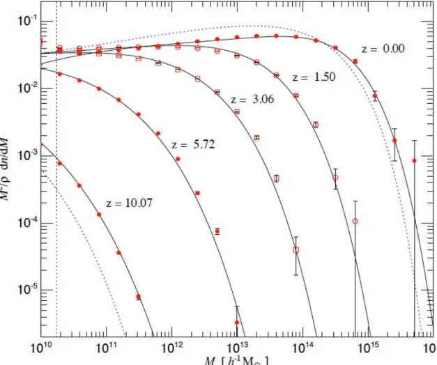
1.7.3 Mass function of dark matter haloes . . . 29
1.7.4 Density profiles of dark matter haloes . . . 30
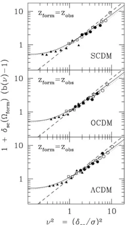
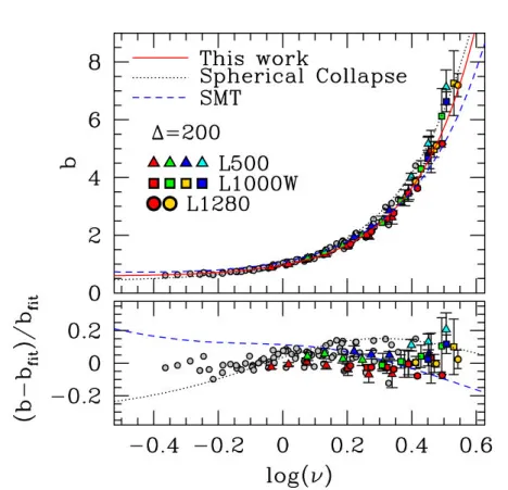
1.8 Analytic approach towards studying the spatial distribution of haloes . . . 32
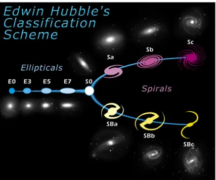
2 What, why and how: Galaxy clusters 39 2.1 Galaxies and galaxy clusters: A brief introduction . . . 39
2.2 Detecting a galaxy cluster . . . 42
Contents
2.2.2 X-ray wavelength detection . . . 43
2.2.3 Sunyaev-Zel’dovich effect . . . 44
2.3 Measuring the mass of a galaxy cluster: Direct measurements and mass proxies 45 2.3.1 Hydrostatic equilibrium: Galaxy clusters . . . 45
2.3.2 Virial theorem . . . 46
2.3.3 Direct methods of mass measurements: X-ray, optical and lensing masses . . . 48
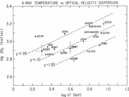
2.3.4 Thermal structure of the ICM . . . 49
2.3.5 Mass proxies: Mass observable relations. . . 50
3 Galaxy and cluster clustering 53 3.1 Methodology: Quantifying structures . . . 53
3.1.1 Definition of the correlation function . . . 53
3.1.2 Different estimators of the correlation function . . . 54
3.1.3 Power spectrum . . . 55
3.1.4 Angular two-point correlation function. . . 56
3.2 Redshift-space distortions: Effect on the correlation function . . . 57
3.3 Galaxy correlation function, a brief review: Angular and spatial correlations 59 3.4 Cluster correlation function, a brief review: Angular and spatial correlations 63 4 Cosmology using galaxy clusters 71 4.1 Using the brightest central galaxies as standard candles . . . 71
4.2 Mass function of galaxy clusters . . . 73
4.3 Galaxy cluster counts . . . 74
4.4 Combining clustering with number counts: Self-calibration approach. . . 79
4.5 Cosmology using baryon acoustic oscillations (BAO) . . . 82
5 Halo clustering: Results from cosmological simulation 87 5.1 Cosmological simulations . . . 87
5.2 The simulation used in this thesis . . . 89
5.3 Calculating the two-point correlation function: Cosmological redshift sample 92 5.3.1 Creating the random catalogue . . . 92
5.3.2 Error estimation . . . 93
5.4 Redshift evolution of the correlation function. . . 94
5.5 Mass evolution of the correlation function . . . 98
5.6 Bias: Evolution with mass and redshift . . . 102
5.7 The r0 vs d relation . . . 110
5.8 Conclusions from this chapter . . . 114
6 Towards clustering of clusters from observational catalogues 117 6.1 Introduction . . . 118
Contents
6.2.1 Modelling of the errors associated with cluster redshifts . . . 119
6.2.2 Recovering the real-space correlation function: Deprojection method 122 6.2.3 Photo-z selection . . . 124
6.2.4 Weighting scheme for photometric redshifts . . . 127
6.2.4.1 Tests performed before calculating the two-point correla-tion funccorrela-tion using weights . . . 130
6.2.4.2 Two-point correlation function from weighted photomet-ric redshifts . . . 132
6.2.5 Real-space correlation function obtained from the deprojection method133 6.2.5.1 Selecting the integration limits . . . 133
6.2.5.2 The quality of the recovery . . . 134
6.2.5.3 Recovering the redshift evolution of the correlation func-tion from sub-samples selected using photometric redshifts139 6.2.5.4 Calculating the bias for the photometric redshift samples . 142 6.2.6 Effects of Purity and Completeness on the two-point correlation func-tion . . . 146
6.2.7 Towards the usage of more realistic photo-z errors . . . 149
6.3 Impact of selecting in Richness on the two-point correlation function . . . 151
6.3.1 Richness definition . . . 152
6.3.2 Scatter in the mass-richness relation . . . 155
6.3.3 Two-point correlation function of richness cut samples . . . 157
6.3.4 Combined effect of richness and photometric redshift errors on the two-point correlation function . . . 161
6.4 Application on observational catalogues: CFHTLS survey . . . 164
6.4.1 Creating the random catalogue . . . 165
6.4.2 Two-point correlation function: Richness cut photometric redshift samples. . . 168
6.5 Conclusions from this chapter . . . 168
7 General conclusions and future prospects 171 7.1 Summary of this thesis. . . 171
7.2 Future perspectives . . . 173
A NFW profiles of the haloes in the simulation 175 A.1 Selecting individual clusters from the data . . . 175
A.2 Calculating the distance to the central galaxy . . . 175
A.3 The mass bins and density profiles . . . 176
A.3.1 The mass bin selection . . . 176
Contents
B Luminosity function & selection effects: Malmquist bias, K-correction 183 B.1 Luminosity function . . . 183 B.2 Eliminating the Malmquist bias. . . 184 B.3 K-correction. . . 185
C Paper published 187
Chapter 1
History of the current cosmological
framework
Contents
1.1 Astronomy before and after 1900 . . . . 2
1.2 The expanding Universe . . . . 4
1.2.1 Hubble’s law . . . 5
1.2.2 Big Bang Nucleosynthesis . . . 6
1.2.3 The Cosmic Microwave Background radiation . . . 6
1.3 Theoretical foundation of cosmology . . . . 7
1.3.1 Friedmann-Lemaître-Robertson-Walker metric and Einstein’s equations 8 1.3.2 Friedmann equations . . . 9
1.3.3 Density parameters of the Universe . . . 11
1.3.4 The curvature of the Universe . . . 11
1.4 Distance measurements in cosmology . . . . 13
1.4.1 Comoving distance (line-of-sight) . . . 13
1.4.2 Comoving distance (transverse) . . . 14
1.4.3 Angular diameter distance . . . 14
1.4.4 Luminosity distance . . . 14
1.5 Towards the standard cosmological model . . . . 15
1.5.1 ΛCDM model . . . 16
1.5.2 Modified Newtonian Dynamics: Alternative to dark matter ?. . . 17
1.6 The accelerated expansion of the Universe . . . . 19
1.6.1 Supernova observations . . . 19
1.6.2 Baryon acoustic oscillations . . . 20
1.7 Formation of large-scale structures: Models and formalisms . . . . 23
1.7.1 Linear perturbation theory . . . 23
1.7.2 Non-linear evolution of large-scale structures . . . 25
2 Chapter 1. History of the current cosmological framework
1.7.2.2 Peak formalism and Press-Schechter formalism: Mass
func-tion . . . 26
1.7.3 Mass function of dark matter haloes. . . 29
1.7.4 Density profiles of dark matter haloes. . . 30
1.8 Analytic approach towards studying the spatial distribution of haloes . . . 32
I would like to start this thesis with a chapter that is intended for a general audience giving a brief review of modern cosmology. First we introduce the three pillars of cosmology; the Hubble’s law, the Big Bang Nucleosynthesis and the Cosmic Microwave Background radia-tion followed by some of the theoretical foundaradia-tions of cosmology such as the Friedmann-Robertson-Walker metric and Einstein’s equations. We then move on to distance measure-ments in cosmology which gives the reader some basic information about how various types of distances to extragalactic sources are measured. We also explain the various cosmological models including the current standard ΛCDM cosmological model and how the accelerated expansion of the Universe was discovered. We finish by introducing the theoretical models and formalisms that have been proposed to explain the formation of the large-scale structures in the Universe.
1.1
Astronomy before and after 1900
One of the oldest natural sciences known to man is astronomy dating back to thousands of years. It was perhaps one of the most common subject followed all the way from India and China in the east to prehistoric Europe and Greece in the west.
Some of the most prominent Asian astronomers of the past include Aryabhata from India, who explicitly mentioned that the earth rotates about its axis, Gan de from China who made one of the very first star catalogues. Some of the most prominent European astronomers of the past include Copernicus, who described the heliocentric model of the solar system, Galileo who used telescopes for astronomical observations and was the first to do so. Kepler was the first to attempt to derive mathematical predictions of celestial motions from assumed physical causes. Combining his physical insights with the observations made by Tycho Brahe, he discovered the three laws of planetary motion. It was Isaac Newton who further developed the relation between astronomy and physics through his laws of universal gravitation. Newton was able to explain all know gravitational phenomenon in one theoretical framework which laid many of the foundations of modern physics.
Before the 20th century, astronomical knowledge was limited to our planet Earth, the Sun, the Moon, the planets of the solar system and stars of the Milky Way. People did not know that other galaxies similar to the Milky Way existed and that we were only one among the many galaxies in the Universe. The world had to wait for the 20th century, which is said to have been the golden era of astronomy as we know today.
1.1. Astronomy before and after 1900 3 During the 20th century, the theory of relativity and quantum mechanics, together with the development of large telescopes and new instrumentation, led to a revolution in astron-omy and to the birth of cosmology as a science. Here we highlight some of the major break-throughs that happened during this epoch as far as extragalactic astronomy is concerned.
Until the 19th century people did not know about galaxy clusters or even groups of galaxy clusters. It was William Herschel and Charles Messier who noted strange objects in the sky which they referred to as “nebulae”, especially being common in some parts of the sky than other and particularly in the constellation of Virgo. For a much detailed analysis of these “nebulae” the world had to wait for the work of Wolf, who described the Virgo and Coma clusters of galaxies (Wolf, 1924). It was still not known that these “nebulae” were extragalactic system of stars which were very similar to our Milky Way.
Hubble made observations of these “nebulae” in 1922-1923 and had a convincing proof that these objects were in fact too distant to be part of our Milky Way and were in fact, entire galaxies outside our own. He went on to present his work in the form of a paper in January 1, 1925 in the meeting of the American Astronomical Society. The galaxies and galaxy clusters were no longer “nebulae” and their mystery was revealed. Hubble went on to use the 100 inch Hooker telescope and measured the distances and velocities to these objects. He made use of Cepheids1for closer objects, and magnitude and size comparisons for the more distance
ones.
In 1927 in the Annales de la Société Scientifique de Bruxelles (Annals of the Scientific Society of Brussels) under the title “Un Univers homogène de masse constante et de rayon croissant rendant compte de la vitesse radiale des nébuleuses extragalactiques” (“A homo-geneous Universe of constant mass and growing radius accounting for the radial velocity of extragalactic nebulae”) Georges Lemaître published a report (Lemaître,1927) . In this report, he derived the Hubble’s law (the detailed explanation of which will be given in Section1.2.1), and provided the first observational estimation of the Hubble constant (Belenkiy,2012). He linked the redshift to cosmological expansion and to relativistic cosmological models.
The graph of velocity vs distance for these objects suggested that they were directly pro-portional (Hubble,1929). The gradient obtained from the graph measured 500 km s−1Mpc−1
2. This positive gradient meant that the Universe was smaller in the past, which in other words
meant that the Universe was expanding and this came to be known as the Hubble’s law. Fritz Zwicky applied the virial theorem to the Coma cluster of galaxies in 1937 and found that there was a mass discrepancy. The application of the virial theorem stated that the Coma cluster contained 400 times more mass than that indicated by the “luminous” and visible objects. This phenomenon was explained by an unidentified type of matter called “dark matter” which has still not been directly observed.
1A Cepheid variable is a type of star that pulsates radially, varying in both diameter and temperature and
producing changes in brightness with a well-defined stable period and amplitude.
2Parsec is a unit of length, which is used to measure distances to objects outside our Solar system. 1 Parsec
(pc) is equal to 3.26 light years and Mpc refers to Megaparsec, which is a distance of one million parsecs. Mpc is usually used for measuring distances to galaxies and galaxy clusters.
4 Chapter 1. History of the current cosmological framework Thus astronomy which was restricted to the studies of the Sun, the Moon and the planets in the Solar System extended its reach to the studies of other galaxies similar to our Milky Way and galaxy clusters in the nearby Universe. Observational techniques could help theoretical studies which had predicted several critical concepts such as the expansion of the Universe and the content of the Universe in detail.
1.2
The expanding Universe
How old is the Universe? How did it began? How large is it? What will be the fate of the Universe? These are all questions that we have been asking for several thousands of years. Cosmology is a study that attempts to answer all these questions by making use of both the-oretical studies (which predict certain results based on a few assumptions) and observational studies (that are required to verify the theoretical predictions). Since Georges Lemaître first noted in 1931 that an expanding Universe might be traced back to a single point in time and space where it could all have begun (Lemaître, 1931), astronomers have built on the idea of cosmic expansion. From the start of the early 20th century, scientists have been trying to explain about the beginning of time and the formation of structures as we see them today us-ing several cosmological models. But two theoretical perspectives namely the Steady State theory and the Big Bang theory divided the astronomers in the mid 20th century.
The “steady state theory” was first proposed byHoyle(1948). The main contradicting statement of the steady state theory compared to the Big Bang theory was that there was no beginning of the Universe. The steady state theory stated that the density of the matter in the expanding Universe remains unchanged due to continuous creation of matter. The Universe was said to be expanding and a homogeneous distribution of matter being created at a rate of 10−24baryon/cm3/s, instead of a unique moment of creation as stated in the Big Bang theory. By the end of the 1960s, the steady state theory started to loose its competitiveness as it could not explain certain observations, such as why galaxies were younger at a higher redshift, why there were excessive radio sources at large distances (Ryle and Clarke,1961) and most importantly the Cosmic Microwave Background (CMB) radiation. The Steady State theory received a lot of appreciation until the mid 20thcentury after which several observational and theoretical evidences started to favour the Big Bang theory.
It was in the 1990s thatHoyle et al. (1993) published a modified version of the steady state theory, that was called the “quasi-steady state” (QSSC) theory. This model solved some of the problems that were faced by the steady state theory such as why there were younger galaxies at higher redshifts and why there were excessive radio sources at larger distances. The QSSC model aimed to compete with the Big Bang theory but described the Universe in a different way. Several errors were found out in the QSSC model byWright(1995) who concluded that the QSSC model failed to describe the many observable properties of the Universe.
1.2. The expanding Universe 5 high density and high temperature scale and continues to expand rapidly. After the initial expansion, the Universe cooled sufficiently to allow for the formation of subatomic particles and later simple atoms. Clouds of these primordial elements later coalesced through gravity to form stars and eventually galaxies. According to the Big Bang paradigm, the expansion of the Universe began 13.8 billion years ago, and this is also considered as the age of the Universe. However according to the Big Bang theory, what happened during the early times of the Universe, approximately from 10−43 to 10−11 seconds after the Big Bang, are still subjects of speculation. The laws of physics as we know them could not have existed during this time and it is difficult to imagine how the Universe would have been governed.
The cosmic microwave background radiation that was discovered in 1965 favoured the Big Bang theory, as the Big Bang theory had predicted this radiation even before it was detected. Supernova experiments have went on to prove the accelerated expansion of the Universe, which maybe due to a positive cosmological constant, a time–varying dark energy component or a modified theory of gravity.
There are three pillars of Big Bang theory, namely: • Hubble’s law
• Big Bang Nucleosynthesis
• Cosmic Microwave Background (CMB) radiation
1.2.1
Hubble’s law
The linear relationship between the redshift of galaxies and their distance is given by:
v = H0D (1.1)
where v is the recessional velocity, expressed in km s−1, H0 is the Hubble’s constant3 ,and
Dis the proper distance from the galaxy to the observer which is measured in megaparsecs (Mpc). The value of H0 as measured by several observational methods give a value that is close to 70 km s−1 Mpc−1. For example as measured from the WMAP observations H0 = 69.32± 0.80 km s−1 Mpc−1 (Bennett et al., 2013), as measured from the Planck mission, H0 = 67.80 ± 0.77 km s−1Mpc−1(Planck Collaboration et al.,2014).
Equation1.1is only a local approximation of the relation between redshift and distance, which depends on the adopted cosmological model.
When the value of H0was still uncertain by a factor 2, a normalized conventional Hubble constant h was defined as:
h= H0 100 km s
−1Mpc−1 (1.2)
6 Chapter 1. History of the current cosmological framework and all quantities that depend on its value was expressed in terms of the reduced Hubble constant, h.
The inverse of the Hubble constant is the Hubble time, tH given by: tH ≡ 1
H0 = 9.78 × 10
9h−1yr= 3.09 × 10¹⁷h−1s (1.3) and the speed of light c times the Hubble time gives us the Hubble distance DH given by:
DH ≡ c
H0 = 3000 h
−1Mpc= 9.26 × 1025h−1m (1.4)
1.2.2
Big Bang Nucleosynthesis
Big Bang Nucleosynthesis (BBN) refers to the production of nuclei heavier than hydrogen during the first minutes after the Big Bang. During this period, helium along with lithium, deuterium, and two unstable radioactive isotopes, the hydrogen isotope tritium and beryl-lium isotope berylberyl-lium-7 are said to have been formed. All of the heavier elements up to iron were created by the nuclear cores within stars. The heaviest elements, those heavier then iron were created during supernova explosions (Copi et al.,1995). Current theory pre-dictions and actual observed abundances of elements match very well, so well that BBN is considered the second fundamental pillar of Big Bang theory (Longair,2008). As we know, the beginning of the Universe was a dense quark soup and the temperature was really high. At this point the mean free path of any given particle was tiny and the entire Universe was within thermodynamic equilibrium. Starting with this hot, dense quark soup and moving forward in time the Universe started to cool and expand. However, as it cooled enough even-tually, particles started freezing out of equilibrium when the energy density of the Universe roughly approached their rest mass energy. The first major component to freeze out were the neutrinos and the second major components to freeze out were the photons. When the temperature decreased to a few thousand degrees, neutral atoms could form without being ionized by photons, which did not have enough energy. This process is called “recombina-tion” and radiation could freely propagate through space.
1.2.3
The Cosmic Microwave Background radiation
As the Universe expanded and cooled to the point where the formation of neutral hydrogen was possible, the fraction of free electrons and protons decreased to a few parts as compared to neutral hydrogen. Immediately after, photons decoupled from matter and travelled freely through the Universe without interacting with normal matter and constitute what is observed today as the Cosmic Microwave Background (CMB) radiation. This radiation is strongest in the microwave region of the radio spectrum and hence the name. One of the images of the CMB radiation observed using WMAP is shown in Figure1.1.
These photons that existed during decoupling have been travelling throughout the Uni-verse ever since. But due to the expansion of the UniUni-verse, their wavelengths are stretched,
1.3. Theoretical foundation of cosmology 7
Figure 1.1: The CMB radiation as measured using WMAP which reveals the fluctuations that correspond to the seeds that grew to became galaxies. Image Credits: WMAP CMB radiation(2007)
the same way in which we see a shift in the red part of the spectrum for all objects that are far away from us (Longair,2008). The CMB radiation has a black body spectrum, which as of today is measured at a temperature of 2.72± 0.0005K (Fixsen,2009). The glow of the CMB radiation is isotropic when seen on a large scale. According to the inflation theory, quantum fluctuations were amplified to macroscopic scales during a period of fast and exponential expansion of the Universe. These density fluctuations were responsible for the temperature fluctuations in the CMB. The temperature fluctuations due to the primordial density fluctua-tions were first detected in 1992 by NASA’s Cosmic Background Explorer (COBE) satellite which detected differences in the CMB radiation temperature in directions separated on the sky by 10○at the level of 30µK (Smoot et al.,1992).
1.3
Theoretical foundation of cosmology
Theoretical predictions have always outpaced observational studies in explaining how the Universe might have formed. During the 1900s, when observational techniques were limited to observing objects at very small distances, several cosmological frameworks were being developed, which were later proved via observational studies. One of the key assumptions of modern physical cosmology is the cosmological principle. It is the assumption that the distribution of matter in the Universe is homogeneous4and isotropic5when viewed on a large
4Homogeneity means that the Universe has the same properties in all locations
8 Chapter 1. History of the current cosmological framework scale. It is clear that the Universe does not obey the cosmological principle on the scale of the Solar System, the galaxy and even on larger scales. Galaxy clusters, superclusters and voids reveal a complex large-scale structure. However, it is assumed that the cosmological principle holds on very large scales, and that averaging over very large volumes the statistical properties (e.g. the mean density) are the same. Assuming the cosmological principle and its validity at any time, one can adopt the Robertson-Walker metric which describes a homogeneous and isotropic Universe and derive the Friedmann equations from the Einstein equations.
1.3.1
Friedmann-Lemaître-Robertson-Walker metric and Einstein’s
equa-tions
The physical distance between points in 3D space (x= (x1, x2, x3)) that has a uniform ex-pansion and growing with time is given by:
∆s2= a2(t)[∆x2 1+ ∆x 2 2+ ∆x 2 3] (1.5)
where a(t) is the scale factor which measures the rate of expansion and is only a function of time t and ∆s gives us the spatial distance between the points. As the expansion of the Universe is uniform, the real distance between the two points Ð→r and the comoving distance (which does not change) Ð→x is given by:
Ð→r = a(t)Ð→x (1.6)
The Hubble parameter H as we have seen can be written in terms of the scale factor as: H≡ ˙a(t)
a(t) (1.7)
where the dot represents the first time derivative. In Equation 1.5 ∆s gives us only the spatial distance between the two points, whereas in general relativity we are interested in the distance between the two points in four-dimensional space, which includes time as the fourth dimension. In that case, the separation between the points is written as:
ds2= ∑ µ,ν
gµνdxµdxν (1.8)
where gµν is the metric and µ and ν are the indices taking the values 0, 1, 2, and 3, x0 is the time coordinate and x1, x2and x3are the three spatial coordinates. The most general spatial metric with constant curvature is written as:
ds23 = dr2 1− kr2 + r
2(dθ2+ sin2θdφ2) (1.9)
where ds2
3 refers to the spatial dimensions alone. The curvature of space is given by k and the possibilities of k being positive, negative and zero correspond to the three different ge-ometries of the Universe. The three common choices for k are:
1.3. Theoretical foundation of cosmology 9 • k= 1, Universe is closed
• k= 0, Universe is flat • k= −1, Universe is open
Adding time dependency to Equation 1.9, we get the Friedmann-Lemaître-Robertson-Walker (FLRW) metric which is given by:
ds2 = −c2dt2+ a2(t)[ dr 2 1− kr2 + r
2(dθ2+ sin2
θdφ2)] (1.10)
where the time coordinate is given by the term dt. This metric according to Einstein’s equa-tion which is given as:
Rµν−1
2gµνR= 8πG
c4 Tµν (1.11)
where Tµνis the energy-momentum tensor of any matter, Rµν and R are the Ricci tensor and scalar which give the curvature of space-time, tell us how the presence of matter and energy curves space-time.
1.3.2
Friedmann equations
The Friedmann equations are one of the most important equations in cosmology as it governs the expansion of space in a homogeneous and isotropic Universe. They were first derived by Alexander Friedmann in 1922 from Einstein’s field equations of gravitation for the FLRW metric and a perfect fluid with a given density ρ and pressure p. This equation has different solutions with different assumptions concerning the material content of the Universe. The first Friedmann equation is given by:
(a˙a)2 = 8πG3 ρ−kc 2 a2 +
Λ
3 (1.12)
where G is Newton’s gravitational constant, ρ is the density, c is assumed to be 1, k is a constant throughout a particular solution, k/a2 is the spatial curvature at any time of the Universe and Λ is the cosmological constant.
It was found out that the Universe not only expands, but at an increasing rate. In cosmo-logical terms this would mean that the cosmic scale factor a(t) which is a function of time has a positive second derivative, so that the velocity of a distant galaxy with respect to the observer is increasing with time. The acceleration of the scale factor is given by the second Friedmann equation: ¨ a a = − 4πG 3 (ρ + 3p c2) + Λ 3 (1.13)
10 Chapter 1. History of the current cosmological framework where p is pressure of the material in the Universe. This equation is called as the acceler-ation equacceler-ation. A positive cosmological constant gives a positive contribution to ¨a and so acts as a repulsive force to gravity. If the cosmological constant is sufficiently large, it can overcome the gravitational attraction represented by the first term of Equation1.13and lead to an Universe which is accelerating. We will see more in detail about the acceleration of the Universe in Section1.6.
One of the most important and often used term in extragalactic astronomy is redshift. When light emitted from an object is increased in wavelength, or shifted to the red end of the spectrum, redshift occurs. In other words one can also say that the frequency of the object decreases as wavelength and frequency are inversely proportional. The wavelength of electromagnetic waves increase proportionally with the scale factor:
λobs λrest =
a(tobs) a(trest)
(1.14) where a(tobs) and a(trest) refer to the scale factors now and then respectively. This implies that the light is redshifted. Redshift can be defined as the change in this wavelength divided by the wavelength the object would have had if it were not moving (i.e. if it were at rest):
z =λobs− λrest
λrest (1.15)
where z is the redshift, λobs is the observed wavelength and λrest is the wavelength of the object at rest.
Redshift does not occur explicitly due to just the expansion of the Universe, it can also occur due to the movement of objects (galaxies and galaxy clusters) relative to each other and also due to gravity, which happens when light is shifted due to the massive amount of matter inside a galaxy.
The movements of objects relative to each other create “peculiar” velocities (vpec), due to which there are differences between an objects measured redshift zobs and it’s cosmological redshift zcos. Cosmological redshifts are those redshifts which are only due to the expansion of the Universe. The relation between the observed redshift zobs, the cosmological redshift zcosand the peculiar redshift (zpec, redshift caused by peculiar velocity) is given by:
1+ zobs = (1 + zcos)(1 + zpec) (1.16)
The reason redshift is one of the most important observable is because most of the distances to extragalactic sources are measured via the redshift, and distance as we know is a primary information that is needed to study any astronomical source.
1.3. Theoretical foundation of cosmology 11
1.3.3
Density parameters of the Universe
It is useful to define the parameter Ω as the ratio of the density (of matter, or radiation, or other components) over the critical density. The critical density is the density value for which the geometry of the Universe is flat(k = 0). The critical density of the Universe is given by:
ρcritical(t) = 3H 2(t)
8πG (1.17)
and it’s value today is given by (Liddle,2003):
ρcritical,0= 3H 2 0(t)
8πG = 1.86 × 10
−29h2g cm−3 (1.18)
where H0denotes the value of the Hubble constant today.
The mass density ρm of the Universe is usually written in terms of a dimensionless pa-rameter ΩM given by:
ΩM ≡8πGρ0 3H2
0
(1.19) and the cosmological constant Λ (explained in detail in Section1.5.1) in terms of a dimen-sionless parameter ΩΛgiven by:
ΩΛ≡ Λc 2 3H2
0
(1.20) Here the subscripted “0” indicates that the quantities (which evolve with time) are to be taken to be at the present epoch. There is a third density parameter, which defines the “curvature” of the Universe denoted by Ωk. Together, these three density parameters are given by:
ΩM + ΩΛ= 1 − Ωk (1.21)
ΩM denotes the mass density including ordinary mass (baryonic mass) and dark matter, ΩΛ denotes the effective mass density of dark energy and Ωk denotes the curvature of the Universe. The values assessed by WMAP (Komatsu et al., 2011) for these parameters are ΩM,0= 0.27 ± 0.04 and ΩΛ,0= 0.725 ± 0.016 and that assessed byPlanck Collaboration et al. (2016) are ΩM,0= 0.31 ± 0.014 and ΩΛ,0= 0.691 ± 0.006
1.3.4
The curvature of the Universe
As we have seen from Equation1.9the Universe can have three possible curvatures depend-ing on the value of k:
• Flat – angles of a triangle add up to 180o
12 Chapter 1. History of the current cosmological framework
Figure 1.2: The local geometry of the Universe is determined by whether the density param-eter Ω is greater than, less than, or equal to 1. From top to bottom: a spherical Universe with Ω > 1, a hyperbolic Universe with Ω < 1, and a flat Universe with Ω = 1. Note that these depictions of two-dimensional surfaces are merely easily visualisable analogues to the 3-dimensional structure of (local) space. Image Credits: Curvature of the Universe(2016)
• Negatively curved (Hyperbolic Universe) – angles of a triangle add up to less than 180o The flat curvature is what we are common with, i.e. Euclidean geometry, wherein the angles of a triangle add up to 180o. The other two geometries are often referred to as Non-Euclidean geometries. An example of a positively curved geometry would be the surface of the Earth. If we were to draw a triangle starting from the equator down to two points in the southern hemisphere, one can notice that the sides of the triangle do not look like a straight line at that particular surface. If the angles are added up, they will be exceeding 180o. An example of a negatively curved space is a horse saddle. The same triangle experiment if repeated on the saddle would lead to the angles of the triangle adding up to less than 180o.
Any Universe with the critical density is said to be flat. There are three cases which lead to different states of the Universe depending on the value of the mass density ρmwith respect to ρcritical:
• If ρm> ρcritical, then the Universe is a closed one, which will eventually stop expanding and start collapsing in on itself.
1.4. Distance measurements in cosmology 13 • If ρm = ρcritical, the the Universe is a flat one, and it will expand forever, but with
decrease in the rate of expansion with time.
In the case of the geometry of the Universe, general relativity explains us that space and time can be bent by mass and energy. This bending of space and time in the Universe decides the curvature and it can be explained via the density parameter Ω of the Universe. As we have seen in Equation1.21, the three density parameters add up to 1, this means that the Universe as we know it, is said to be flat, which is the first scenario. If Ω on the other hand is greater than 1, it means that there is positive curvature, and if Ω is less than 1, there is negative curvature.
1.4
Distance measurements in cosmology
Due to the expansion of the Universe, the distances between comoving objects are changing, which means that there are many ways to specify the distance between two points in space. When we look at objects far far away we are literally looking back in time. One of the main ingredient from which distances to far away objects are measured is the redshift of that object. Once we have the redshift of the object, measured either using photometry or spec-troscopy and the values of our three cosmological parameters, we can calculate the distance to the object. Here we will explain some of the major distance measures used in cosmology, which include the comoving distance (line-of-sight/transverse), angular diameter distance and the luminosity distance.
1.4.1
Comoving distance (line-of-sight)
If we need to calculate the distance to an object which is stationary, we can directly do so. The same applies to distant objects in space, i.e. if we need to calculate the distance to an extragalactic source at a specific moment of cosmological time, which is called as proper distance, it can be calculated. But we know that the Universe is expanding, so, the far away an object is, the faster it expands from us. Comoving distance factors out this expansion, and gives us a distance that does not change with time. At the present epoch, both comoving distance and proper distance are one and the same, but at other times, they aren’t.
The total line-of-sight comoving distance DC from us to a distant object is calculated by summing up (integrating) all the small δDC contributions in between the line-of-sight direction. We define a function E(z) as:
E(z) ≡√ΩM(1 + z)3+ Ω
k(1 + z)2+ ΩΛ (1.22)
and the total line-of-sight comoving distance is then given by: DC = DH∫
z
0 dz′
14 Chapter 1. History of the current cosmological framework where DH is the Hubble distance given by Equation1.4. There are other distance measures such as Luminosity distance, Parallax distance, Angular diameter distance, etc. but all the above distances are based on the comoving distance in one way or the other (Hogg, 1999). In other words, the fundamental distance measure in cosmology is the comoving distance.
1.4.2
Comoving distance (transverse)
The distance between two objects in the sky at the same redshift or distance but separated on the sky by some angle δθ is DMδθand the transverse comoving distance DM, related to the line-of-sight comoving distance is given by:
DM =⎧⎪⎪⎪⎪⎪⎨ ⎪⎪⎪⎪⎪ ⎩ DH√1 Ωksinh[ √ ΩkDC/DH] for Ωk> 0 DC for Ωk= 0 DH√1 ∣Ωk∣ sin[√∣Ωk∣DC/DH] for Ωk< 0 (1.24)
where the functions sinh and sin account for the curvature of space. For ΩΛ = 0, there is an analytic solution to the equations:
DM = DH 2[2 − ΩM(1 − z) − (2 − ΩM) √ 1+ ΩM(z)] Ω2 M(1 + z) for ΩΛ= 0 (1.25)
1.4.3
Angular diameter distance
The angular diameter distance DAis defined as the ratio of an object’s physical transverse size to its angular size (in radians) (Hogg,1999). DAdoes not increase indefinitely as z → ∞; it turns over at z∼ 1 and so more distant objects actually appear larger in angular size. DA is related to DM by:
DA= DM
1+ z (1.26)
1.4.4
Luminosity distance
The luminosity distance DL is defined as the relationship between bolometric6 flux S and bolometric luminosity L and is given by:
DL≡ √
L
4πS (1.27)
It can also be given in terms of the transverse comoving distance and angular diameter dis-tance by:
1.5. Towards the standard cosmological model 15
DL= (1 + z)DM = (1 + z)2DA (1.28)
This relation follows from the fact that surface brightness of a receding object is reduced by a factor(1 + z)−4and the angular area is reduced by D−2
A (Hogg,1999).
1.5
Towards the standard cosmological model
The development of a standard model of cosmology has been going on for the last forty years. The most widely accepted model is the ΛCDM model which can explain some of the observable properties of galaxies, clusters and large-scale structures in the Universe. Pre-dictions of the ΛCDM model on the distribution of galaxies both nearby and out to high redshifts have been confirmed by observations (Komatsu et al., 2009;Planck Collaboration et al., 2015), although on sub-galactic scales there are several potential problems such as the model predicting an excess of halo substructures with respect to the observed number of satellite galaxies. But before the ΛCDM model became the standard model, there were several other models that were competing.
It was during the early 1980s that scientists were proposing that dark matter could be composed of non-baryonic particles. The candidate dark matter particles were classified into three families: hot, warm and cold dark matter (CDM), names that reflected their typi-cal velocities during the early time of the Universe (Bond et al.,1980). Light neutrinos were considered as the Hot Dark Matter (HDM) candidates (Ellis et al., 1984). The CDM and HDM models with different ΩM values were compared with the spatial distribution of galax-ies observed from the CfA survey (Efstathiou et al., 1985). The results showed that there was discrepancy in the HDM models when compared with the results from the CfA survey while on the other hand the CDM models gave a far better result when compared to the CfA data. Studies on simulations based on CDM initial conditions were compared with the CfA galaxy distribution with predictions for a high-density Einstein de Sitter (EdS) Universe and with predictions for a low density Universe byDavis et al.(1985a). It was found out byDavis et al.(1985a) that a ΩM ∼ 0.4 gave convincing results.
In the 1980s a flat Universe was considered as the outcome of inflation and a biased EdS model called the “standard” Cold Dark Matter (SCDM) model became the preferred choice for several investigations using N-body simulations (Frenk et al.,1985;White et al., 1987). The SCDM model was characterised by: h = 0.5, ΩB = 0.05 and ΩM = 0.95 (Dodelson
et al.,1996). The SCDM model showed success at forming galaxies and cluster of galaxies, but problems remained, as the model required a Hubble constant that was lower than that preferred by observations. It was in the early 1990s that it had become clear that galaxy correlations were stronger on large scales than predicted by SCDM. The transition to ΛCDM model was finally forced by the exclusion of the EdS expansion history by supernova data (Perlmutter et al.,1999), which showed an accelerated expansion of the Universe.
16 Chapter 1. History of the current cosmological framework
1.5.1
ΛCDM model
The current standard model in which the Universe contains the cosmological constant Λ is called as the ΛCDM model. It is the simplest model that can reproduce the observational properties of the Universe such as:
1. The properties of the CMB radiation, as the existence of CMB is predicted by any Big Bang model.
2. The large-scale structure evolution and its distribution.
3. The accelerated expansion of the Universe, as given by the term Λ (cosmological con-stant) from ΛCDM.
The present composition of the Universe is:
• Baryonic matter: Roughly 5% of the Universe is ordinary baryonic matter Ωb, mainly made up of Hydrogen atoms, Helium atoms and other fractions of heavier elements. • Dark matter: Roughly 25% of the Universe is in the form of unknown dark matter,
made up of particles that interact with ordinary matter only via the force of gravity. • Dark energy: The remaining∼ 70% is in the form of unknown dark energy ΩΛ, which
is responsible for the acceleration of the Universe as we have observed today.
Figure 1.3: A pie-chart representing the matter-energy content of the Universe. Credits:
1.5. Towards the standard cosmological model 17 The dominant component of the Universe is the dark energy. However, there are other possibilities, such as a new form of energy which could evolve with time (quintessence), or a modified theory of gravity. Results from observational analysis that is model-independent can give us the proper solution, but at the moment the observational data are not up to the mark to take up this task. So we have to use the available data to constrain the model pa-rameters. The most common way of discriminating between a cosmological constant and dynamical dark energy is to make use of the dark energy equation-of-state parameter, which in terms of the scale factor a is given as:
w(a) = w0+ wa(1 − a) (1.29)
It can be seen that at the present time (a= 1) w(a) = w0. The cosmological constant corre-sponds to w0 = −1 and wa= 0, constant equation of state corresponds to w0 = w = constant and wa = 0, whereas the case of dynamical dark energy corresponds to wa ≠ 0. The dif-ference between Λ and dynamical dark energy is that the former is constant with time and space, whereas the latter can change in time and space.
1.5.2
Modified Newtonian Dynamics: Alternative to dark matter ?
The dark matter component of the Universe was first detected using the rotation curves of galaxies, which was found to not follow the Keplerian decline with radius. Newton’s law predict that stellar rotation velocities should decrease with distance from the galactic cen-tre. The very first detections were done in 1930s when Horace Babcock reported the mea-surements of the rotation curve of the nearest Andromeda galaxy which suggested that the mass-to-luminosity ratio increases radially (Babcock,1939). But detailed analysis of these measurements were done in 1970s by Vera Cooper Rubin and her team who measured the velocity curves of several stars in edge-on spiral galaxies. One such example is given in Fig-ure1.4which shows that the velocity of the spiral galaxy NGC 6503 does not decline with radius but remains a constant. These observations showing the discrepancy in the rotational velocity curve meant that either there existed some form of unknown excess matter in the galaxies which boost the velocities of stars, or Newton’s law does not apply to galaxies. The first statement lead to the dark matter hypothesis and the second statement lead to Modi-fied Newtonian Dynamics (MOND) model, created by Milgrom (Milgrom, 1983), which is based on a variation of the Newton’s Second Law of dynamics at low accelerations. MOND is closer to the main characteristics of the standard model, but different in minor aspects. According to Milgrom (1983) the discrepancy could be resolved if the gravitational force experienced by a star in the outer regions of a galaxy was proportional to the square of its centripetal force unlike to the centripetal force itself as given by Newton’s second law.The basic concept of MOND was that Newton’s laws were tested in high-acceleration environment, but have not been verified for objects with low acceleration, such as the stars in the outer parts of a galaxy. According to MOND, the Newtonian force is given by:
18 Chapter 1. History of the current cosmological framework
Figure 1.4: Rotation curve for the spiral galaxy NGC6503. The points are the measured circular rotation velocities as a function of distance from the center of the galaxy. The dashed and dotted curves are the contribution to the rotational velocity due to the observed disk and gas, respectively, and the dot-dash curve is the contribution from the dark halo. Credits:
Kamionkowski(1998)
FN = mµ (a
a0)a (1.30)
where FN is the Newtonian force, m is the object’s gravitational mass, µ(x) is an as-yet unspecified function (known as the “interpolating function”), a is the acceleration and a0is a new fundamental constant which marks the transition between Newtonian and deep-MOND regimes. To agree with Newtonian mechanics requires µ(x) → 1 for x ≫ 1 and to agree with astronomical observations requires µ(x) → x for x ≪ 1.
The strongest success of MOND is that all the rotation curves of galaxies imply a unique universal value for acceleration; moreover, the rotation curve features feel the baryonic com-ponent features even where dark matter is dominant; and in general the observed acceleration is strictly correlated with the acceleration expected from baryonic matter (McGaugh et al.,
2016;Milgrom,2016). On the other hand, MOND does not completely eliminate the need for a dark matter component, as galaxy clusters show a residual mass discrepancy even when analysed using MOND (McGaugh,2015).
1.6. The accelerated expansion of the Universe 19
1.6
The accelerated expansion of the Universe
As we discussed in Section1.1 the discovery of a linear proportionality between velocities and distances of galaxies along with the discovery of the CMB in 1965, paved the way to the acceptance of an expanding Universe. In the end of 90s, physicists were convinced that the force of gravity should be causing the expansion of the Universe to slow down. But the first evidence to favour the accelerated expansion of the Universe came from supernova observations. This meant that the scale factor had a positive second derivative.
There have been several observational evidences in favour of the accelerated expansion of the Universe. One can either look at the magnitude-redshift relation of objects that are “standard candles”7or use the baryon acoustic peak measurements as “standard rulers”. As
discussed above, we highlight here how the two methods paved the way towards understand-ing the acceleration of the Universe.
1.6.1
Supernova observations
The first direct evidence of the accelerated expansion of the Universe came from supernova observations, in particular Type Ia supernovae (SNIa). These are white dwarfs that explode because they exceed the Chandrasekhar limit 8. The peak brightness of the supernova is
found using repeated observations from which we can infer the luminosity distance, which is associated with the redshift of the host galaxy. The measured luminosity distance can then be compared with theoretical predictions to constrain the values of ΩM and ΩΛto distinguish between several cosmological models.
Mario Hamuy (Hamuy et al., 1993) and co-workers at Cerro Tololo took a major step for-ward by studying the light curves of many nearby supernovae. But it was in 1998 that Saul Perlmutter heading the Supernova Cosmology Project (SCP) along with the High-z Super-nova Search Team measured the brightness of 42 superSuper-novae and compared their magnitude with redshift. In Figure1.5we show the redshift vs magnitude diagram obtained from SNIa observations from the Supernova Cosmology Project and the High-z Supernova Search on a logarithmic redshift scale. Here they compared the SNIa observations to a few cosmological models and found out that the observations do not match the Λ= 0 model and favours the model with Λ > 0 (Perlmutter et al., 1999). This discovery was named as “Breakthrough of the year for 1998” with Perlmutter alongside Adam Riess and Brian P.Schmidt from the High-z team being awarded the Nobel Prize in Physics. Supernovae also provide precise measurements of the Hubble parameter H0. One of the recent works byRiess et al.(2011) obtained a value of H0 = 73.8 ± 2.4kms−1Mpc−1.
7Those astronomical objects that have a known brightness, so by comparing this known brightness to the
observed brightness, one can determine the distance to the object using inverse square law.
8Any white dwarf that reaches a mass above M
20 Chapter 1. History of the current cosmological framework
Figure 1.5: Observed magnitude versus redshift is plotted for well-measured distant and (in the inset) nearby type Ia supernovae. For clarity, measurements at the same redshift are combined. At redshifts beyond z = 0.1 (distances greater than about 109 light-years), the cosmological predictions (indicated by the curves) begin to diverge, depending on the assumed cosmic densities of mass and vacuum energy. The red curves represent models with zero vacuum energy and mass densities ranging from the critical density ρc down to zero (an empty cosmos). The best fit (blue line) assumes a mass density of about ρc
3 plus a vacuum energy density twice that large–implying an accelerating cosmic expansion. Credits: (Perlmutter,2003)
1.6.2
Baryon acoustic oscillations
As SNIa provide a “standard candle”, BAO clustering information can provide a “standard ruler” for length scale in cosmology.
The early Universe consisted of a hot plasma and the photons as we know were trapped and were not able to travel any considerable distance before interacting with this plasma. There were over dense regions of this plasma which attracted matter towards it gravitation-ally. This attraction lead to a high temperature region and in-turn creating a high pressure region. The counteracting forces of gravity and pressure created oscillations, analogous to
1.6. The accelerated expansion of the Universe 21
Figure 1.6: The two-point correlation function of a sample of SDSS luminous red galaxies as calculated byEisenstein et al. (2005). The BAO peak is spotted at around 105 h−1Mpc. Credits: Eisenstein et al.(2005)
sound waves created in air by pressure differences. Photons along with protons and electrons remained trapped in this high pressure region until the Universe expanded and cooled. When the temperature finally reduced, the photons were set free and started moving but the elec-trons and protons (baryonic matter) stopped moving and remained at the center of this high pressure region. This left behind a shell of baryonic matter at a fixed radius which can be statistically detected through the two-point correlation function ξ(r). ξ(r) decreases with in-creasing scale, but we observe a slight increase in ξ(r) at a particular scale. This scale is the fixed radius where the baryonic matter can be found in excess. An example of the BAO peak measured from the two-point correlation function of LRGs from the SDSS sample by Eisen-stein et al.(2005) is shown in Figure1.6. It can be seen that this peak is more or less around 105 h−1Mpc. In understanding the accelerated expansion of the Universe, observations of the sound horizon today (using clustering of galaxies) can be compared with the sound hori-zon at the time of recombination (using CMB). BAO thus provides a “standard ruler” and a way to understand this expansion completely independent from SNIa observations. Eisen-stein et al.(2005) quoted the distance measurement as a combination of the line-of-sight and transverse distance scale given by: