HAL Id: tel-01287729
https://hal.archives-ouvertes.fr/tel-01287729
Submitted on 14 Mar 2016
HAL is a multi-disciplinary open access
archive for the deposit and dissemination of
sci-entific research documents, whether they are
pub-L’archive ouverte pluridisciplinaire HAL, est
destinée au dépôt et à la diffusion de documents
scientifiques de niveau recherche, publiés ou non,
transportation networks
Paolo Bajardi
To cite this version:
Paolo Bajardi. Epidemic spreading : the role of host mobility and transportation networks. Statistical
Mechanics [cond-mat.stat-mech]. Aix Marseille Université, 2011. English. �tel-01287729�
Diffusion des ´
epid´
emies:
le role de la mobilit´
e des agents et des r´
eseaux de
transport
Epidemic spreading:
the role of host mobility and transportation networks
Th`ese pr´esent´ee par
Paolo Bajardi
pour obtenir le grade de
Docteur d’Aix-Marseille Universit´e
Sp´ecialit´e: Physique Th´eorique et Math´ematique Ecole Doctorale de rattachement: Physique et Sciences de la Mati`ere
`
A soutenir le 24 Novembre 2011 devant le jury compos´e de:
A. Barrat F. Carrat V. Colizza P. Jensen R. Pastor-Satorras J.-F. Pinton Directeur de Th´ese Rapporteur Co-directrice de Th´ese Rapporteur Membre du Jury Membre du Jury
Ces derni`eres ann´ees, la puissance croissante des ordinateurs a permis `a la fois de rassembler une quantit´e sans pr´ec´edent de donn´ees d´ecrivant la soci´et´e moderne et d’envisager des outils num´eriques capables
de s’attaquer `a l’analyse et la mod´elisation les processus dynamiques qui se d´eroulent dans cette r´ealit´e
complexe. Dans cette perspective, l’approche quantitative de la physique est un des catalyseurs de la
croissance de nouveaux domaines interdisciplinaires visant `a la compr´ehension des syst`emes complexes
techno-sociaux. Dans cette th`ese, nous pr´esentons dans cette th`ese un cadre th´eorique et num´erique pour simuler des ´epid´emies de maladies infectieuses ´emergentes dans des contextes r´ealistes. Dans ce but, nous
utilisons le rˆole crucial de la mobilit´e des agents dans la diffusion des maladies infectieuses et nous nous
appuyons sur l’´etude des r´eseaux complexes pour g´erer les ensembles de donn´ees `a grande ´echelle d´ecrivant
les interconnexions de la population mondiale. En particulier, nous abordons deux diff´erents probl`emes de sant´e publique. Tout d’abord, nous consid´erons la propagation d’une ´epid´emie au niveau mondial, et pr´esentons un mod`ele de mobilit´e (GLEAM) con¸cu pour simuler la propagation d’une maladie de
type grippal `a l’´echelle globale, en int´egrant des donn´ees r´eelles de mobilit´e dans le monde entier. La
derni`ere pand´emie de grippe H1N1 2009 a d´emontr´e la n´ecessit´e de mod`eles math´ematiques pour fournir des pr´evisions ´epid´emiques et ´evaluer l’efficacit´e des politiques d’interventions. Dans cette perspective, nous pr´esentons les r´esultats obtenus en temps r´eel pendant le d´eroulement de l’´epid´emie, ainsi qu’une analyse a posteriori portant sur les strat´egies de lutte et sur la validation du mod`ele. Le deuxi`eme
probl`eme que nous abordons est li´e `a la propagation de l’´epid´emie sur des syst`emes en r´eseau d´ependant
du temps. En particulier, nous analysons des donn´ees d´ecrivant les mouvements du b´etail en Italie afin de caract´eriser les corr´elations temporelles et les propri´et´es statistiques qui r´egissent ce syst`eme. Nous ´etudions ensuite la propagation d’une maladie infectieuse, en vue de caract´eriser la vuln´erabilit´e
du syst`eme et de concevoir des strat´egies de contrˆole. Ce travail est une approche interdisciplinaire qui
combine les techniques de la physique statistique et de l’analyse des syst`emes complexes dans le contexte de la mobilit´e des agents et de l’´epid´emiologie num´erique.
In recent years, the increasing availability of computer power has enabled both to gather an unprecedented amount of data depicting the global interconnections of the modern society and to envision computational tools able to tackle the analysis and the modeling of dynamical pro-cesses unfolding on such a complex reality. In this perspective, the quantitative approach of Physics is catalyzing the growth of new interdisciplinary fields aimed at the understanding of complex techno-socio-ecological systems. By recognizing the crucial role of host mobility in the dissemination of infectious diseases and by leveraging on a network science approach to handle the large scale datasets describing the global interconnectivity, in this thesis we present a theo-retical and computational framework to simulate epidemics of emerging infectious diseases in real settings. In particular we will tackle two different public health related issues. First, we present a Global Epidemic and Mobility model (GLEaM) that is designed to simulate the spreading of an influenza-like illness at the global scale integrating real world-wide mobility data. The 2009 H1N1 pandemic demonstrated the need of mathematical models to provide epidemic forecasts and to assess the effectiveness of different intervention policies. In this perspective we present the results achieved in real time during the unfolding of the epidemic and a posteriori analysis on travel related mitigation strategies and model validation. The second problem that we address is related to the epidemic spreading on evolving networked systems. In particular we analyze a detailed dataset of livestock movements in order to characterize the temporal correlations and the statistical properties governing the system. We then study an infectious disease spreading, in order to characterize the vulnerability of the system and to design novel control strategies. This work is an interdisciplinary approach that merges statistical physics techniques, complex and multiscale system analysis in the context of hosts mobility and computational epidemiology.
1 Introduction 1
2 Theoretical Framework: Networks and Graphs 5
2.1 Basic definitions . . . 6 2.2 Real networks . . . 9 2.2.1 Social networks . . . 9 2.2.2 Technological networks . . . 9 2.2.3 Biological networks . . . 10 2.3 Network models . . . 10
2.3.1 Random networks: Erd¨os-R´enyi (ER) model . . . 10
2.3.2 Small world networks: Watts-Strogatz (WS) model . . . 12
2.3.3 Scale free networks: Barab´asi-Albert (BA) model . . . 13
2.4 Dynamical networks . . . 15
2.5 Conclusions . . . 15
3 Theoretical Framework: Epidemic Models 17 3.1 Compartmental models . . . 18
3.2 Epidemic spreading on graphs . . . 23
3.3 Metapopulation models . . . 25
3.4 Conclusion . . . 27
4 GLobal Epidemic and Mobility model 29 4.1 Global Population and subpopulations definition . . . 30
4.2 World Airport Network . . . 32
4.3 Commuting Networks . . . 32
4.5 Stochastic and discrete integration of the disease dynamics . . . 36
4.6 The integration of the transport operator . . . 37
4.7 Time-scale separation and the integration of the commuting flows . . . 38
4.8 Effective force of infection . . . 40
5 Global spread of H1N1 pandemic influenza 43 5.1 Background . . . 44
5.2 Disease parameters estimation . . . 46
5.3 Real time predictions . . . 55
5.4 Estimating the early number of cases in Mexico . . . 57
5.5 Intervention strategies . . . 60
5.5.1 Vaccination campaign . . . 60
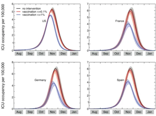
5.5.2 Modeling the critical care demand . . . 67
5.5.3 Travel restrictions . . . 70
5.6 Assessment of model predictions and discussion . . . 84
6 Dynamical network analysis and spreading simulations 87 6.1 Background . . . 89
6.2 Data description . . . 90
6.3 Daily and aggregated networks . . . 93
6.4 Network microscopic dynamics . . . 105
6.4.1 Activity timescales . . . 105
6.4.2 Fluctuations of nodes and links properties . . . 109
6.4.3 Evolution of the network backbone . . . 111
6.4.4 Dynamical motifs . . . 113
6.5 Spreading processes on dynamical networks . . . 116
6.5.1 Percolation analysis . . . 117
6.5.2 Epidemic spreading simulations . . . 119
6.5.3 Invasion paths and seeds’ cluster detection . . . 122
6.5.4 Longitudinal stability of the seeds’ clusters . . . 127
6.5.5 Disease sentinels . . . 129
6.5.6 Generalization to the stochastic case . . . 133
6.6 Conclusions . . . 138
Introduction
Since the mid-20th century, the availability of new computational resources has added novel and important tools to theoretical physics. In particular, statistical mechanics had found in computer simulations the perfect environment to perform numerical experiments to explore ideal systems composed by thousands of interacting elements. Nowadays, the technological innovations have pushed the computational power to an extent unthinkable even twenty years ago. The easiness to which it is possible to perform huge calculations on ordinary personal computers represents a precious opportunity to tackle the study of natural processes involving a multitude of interacting objects in a complex reality, shifting the attention from ideal systems to the real-world phenomena.
Along with the technical innovations, the last decade has witnessed an increasing attention to the data gathering, ranging from biological (1; 2; 3; 4) to social systems (5; 6; 7; 8; 9; 10; 11; 12), from infrastructural (7; 13; 14; 15; 16) to financial realities (17; 18; 19; 20). In particular, the pervasiveness of technology in the every day life allowed physicists to quantitatively explore new fields. For instance, the mobile phones provide informations about the geographical position of his/her owner (21) and can be used as a proxy of human mobility as well as the tracking of banknotes (22). Furthermore, the analysis of mobile communication (23) along with the web 2.0 and the virtual social networks (24) permit the analysis of social interactions at a very large scale considering the interactions among thousand of individuals and measuring the conjectures and the hypothesis proposed by sociologists (25) and anthropologists (26) since the last century. Moreover, research on some technological systems pointed out their tendency to evolve as autonomous systems even though they have been built in their constituent elements by human beings, as in the case of the Internet (27) or the World-Wide-Web (28). All the above
mentioned systems are composed by many interacting entities and in order to formalize such interactions and to conveniently handle them, many datasets have been naturally described in terms of networks. The analysis of such systems highlighted their intrinsically complex nature: their behavior cannot be described extrapolating the properties and the governing laws of their constitutive units. The study of each subpart of the system in isolation does not allow the understanding of the whole system and its dynamics. In many cases, we observe the spontaneous outcomes of emerging phenomena due to the interactions among the system constitutive units. They are self-organizing systems without a blueprint or a global supervision.
The ambitious aim of the new computational science is to understand and predict through a data-driven approach the behavior of large-scale phenomena of the above mentioned techno-social systems. Starting with the mathematical description of patterns found in real data, scientists can devise models to anticipate trends, in order to evaluate risks and eventually manage future events (29). The most successful example of the potential of the computational modeling approach to complex settings is represented by weather forecasts: powerful supercomputers elaborate current meteorological data and correlate with huge libraries of historical entries into large-scale computational simulations achieving extraordinary results. Using the physical laws governing the dynamics of fluid and gas masses and sophisticated equipment to record data at the local level, in the last decades the development of accurate weather forecasts permitted to project the path and intensity of storms, hurricanes, and other disruptive meteorological occurrences and, in many cases, to save thousand of lives by anticipating and preparing for these events. On the other hand, the main obstacle for the understanding of human-related phenomena was the lack of large-scale data about human patterns and consequently the difficulty in formalizing mathematical laws governing human behavior. With the increasing availability of data about the individual and collective human dynamics, we are finally able to study phenomena involving social systems with the quantitative approach of statistical Physics. In this perspective, the modeling of epidemic spreading of infectious diseases is a challenging problem with immediate and important applications related to public health issues. Similarly to weather forecasts, we have to feed with the appropriate data and initial conditions the set of laws governing the transmission of pathogens in a spatially extended systems. The dissemination of infectious diseases is governed by host mobility at different scales. For instance, a child that gets influenza interacting with schoolmates can transmit the disease to her/his parents when s/he comes back home. Subsequently the parents might infect their colleagues at the workplace that is eventually placed in a neighboring town and the infection chain might continue infecting more and more people. In the pre-industrial
Figure 1.1: Disease spreading examples. The slow propagation of the black death in the 14th century (A) is compared with the rapid dissemination at the global scale of the 2009 H1N1 influenza (B).
age the human mobility was characterized by rare travels covering rather short distances, leading to a slow dissemination of new pathogens. As shown in figure 1.1A, it has been estimated that in the 14th century the so-called ’Black Death’ was able to spread at the velocity of few hundreds miles per year. On the contrary, the mobility in the modern society is shaped by the large fluxes of short range daily commuters and air travelers. In such settings the spreading of infectious diseases may rapidly reach global proportions as in the paradigmatic case of the 2009 H1N1 pandemic shown in figure 1.1B. In this thesis, integrating with a network science approach the large-scale datasets describing the host mobility, we present a theoretical and computational framework to simulate epidemics of emerging infectious diseases in real settings.
The thesis is organized as follow. In chapter 2 we recall the basic concepts of graph theory, we introduce some mathematical tools that are necessary to analyze networked systems and we review three models that represent milestones of network science and are useful to understand the behavior of complex networks. In chapter 3 we provide an introduction to mathematical modeling of infectious diseases. The transmission of a pathogen within a host population can be described as a dynamical process governed by a set of differential equations by defining an appropriate phase space. In chapter 4 we describe in detail the Global Epidemic Mobility model (GLEaM) that integrates a data-driven network description of human mobility and an epidemic model of an influenza like illness. The work concerning GLEaM has been carried out within a large collaboration led by Vittoria Colizza (PI) and Alessandro Vespignani (PI and Team Coordinator) based mainly at the I.S.I Foundation, Turin, IT and at the Indiana University, Bloomington, IN, USA. Under the supervision of Vittoria Colizza, I have partially helped in the data gathering and
analysis of short range mobility datasets, while the computational implementation of GLEaM and the numerical simulations of epidemic scenarios has been an important part of the work performed during this thesis and it represents the crossing point of the interdisciplinary merging of human disease modeling, complex networks science and policy decision making. In chapter 5 we present the results obtained by using GLEaM to perform forecasts, analysis and intervention assessments during the 2009 H1N1 pandemic influenza. It is worth to stress that most of those results were achieved well before the epidemic peak opening the road to real time epidemic forecasting. In chapter 6 we present the results achieved under the supervision of Alain Barrat and Vittoria Colizza aimed at the development of novel mathematical and statistical tools through the longitudinal analysis of a dynamical complex network. Many systems are usually treated as static networks mainly because of a lack of information on the timing of the interactions and also because the static description is often a good approximation for several purposes. Nevertheless, when the time scale of the system dynamics is comparable to the investigated dynamical process it is crucial to incorporate the whole temporal information. We thus present the study on a detailed dataset of livestock movements that represents a unique opportunity to define new quantities and physical observables to analyze networked systems with an explicit temporal dimension. Finally, we further discuss some important features that may affect the spreading of an emerging infectious disease and we propose a novel approach to study dynamical processes on dynamical networks.
Theoretical Framework:
Networks and Graphs
Contents
2.1 Basic definitions . . . 6 2.2 Real networks . . . 9 2.3 Network models . . . 10 2.4 Dynamical networks . . . 15 2.5 Conclusions . . . 15The first scientist to introduce the notion of graph was Leonard Euler in the famous work Solutio problematis ad geometriam situs pertinentis in 1736, where he solved the K¨onigsberg bridges problem.
Generally speaking, a graph is an abstract way of specifying relationships among a collection of objects. Such level of abstraction can be applied to a broad range of systems. In this perspec-tive graphs provide a theoretical framework that allows a convenient conceptual representation of interrelations in complex systems where the system characterization implies the mapping of interactions among a large number of constituent elements. The study of graphs has a long tra-dition in discrete mathematics, sociology, and communication research and has recently become very popular also in physics and biology.
In this work, the concept of networks plays a crucial role providing a suitable framework to explore computationally the unfolding of dynamical processes in complex realities and to tackle
theoretical issues raised by the dynamics of the system itself. In this chapter we will introduce the very basic concepts of this field but we refer the reader for a deeper analysis of the subject to some classical books for a more theoretical point of view (30; 31; 32; 33; 34; 35; 36) and for a more applied perspective (27; 37; 38; 39; 40; 41).
2.1
Basic definitions
A graph G(N, E) is identified by a set of N objects named vertices or nodes and a list of E pairs of nodes, called edges or links indicating the relationships between the objects. Two nodes are neighbors if they are connected by an edge. The relationships between the objects can be symmetric or asymmetric leading to undirected or directed graphs respectively. Graphs are useful because they serve as mathematical models of network structures and from now on we will refer to graphs or networks without further distinctions. A convenient way to mathematically describe a graph is through the N× N adjacency matrix A, whose element Aij = 1 if the nodes i and
j are connected and Aij = 0 otherwise. Using such formalism, the undirected networks are
represented by a symmetric adjacency matrix (Aij= Aji), while in the directed cases the matrix
can be asymmetric. Moreover, in the following we will consider only networks without self-loops (Aii = 0). Depending on the system under study, it might be important to add a new degree
of freedom representing the intensity of the relationships between nodes. It is thus possible to construct weighted networks where each connection (i, j) has its own weight wij.
In the following we recall some fundamental concepts and definitions used for the quantitative analysis of complex networks.
Path, connectivity and distance
A path Pij defined in graph G(N, E) is an ordered collection of edges connecting the nodes i
and j. A graph is called connected if for every pair of nodes there is a path between them. A component C is defined as a connected subgraph and two components C1(M1, E1) and C2(M2, E2)
are disconnected if it is impossible to construct a path Pij with i ∈ M1 and j ∈ M2. Graphs
usually lack a metric, but the distance between two vertex can be naturally defined as the number of links traversed by the shortest connecting path. For two given nodes i and j the distance lij
between them is the path length with the minimum number of links between them. If the nodes i and j belong to two disconnected components, their distance is set to infinity. The diameter D of a graph is the maximal distance among all the pairs of nodes.
The average distance L is evaluated averaging the shortest paths for all the possible couples of nodes (i, j): L = 2 N (N− 1) � i<j lij (2.1)
If L is much smaller than the size of the system N , the network is said to exhibit a small world property.
Degree
The degree ki of a node i is the number of links connected to i, i.e. the number of its neighbors.
By using the adjacency matrix formalism ki=�jAij while the average degree is simply�k� =
2E/N . In a directed graph the number of incoming or outgoing connections are called in-degree kinor out-degree koutrespectively. The definition of degree can be generalized to weighted graphs
where the weighted degree is usually called strength. The strength a the node i is si=�jwij,
and similarly to the unweighted directed graphs it is possible to define the in-strength and the out-strength quantities.
Centrality measures
When considering a network, the centrality of the nodes and links is crucial to understand their role in the systems. The degree is one of the simplest and more common centrality measure adopted to assess the node centrality, but many others exists: betweenness node/link centrality, closeness centrality, eigenvector centrality, pagerank. We will not go into details of such measures since in this work we will use the degree whenever we investigate the centrality of a node and we refer the reader to classical textbooks (37; 38; 39; 40) to deepen this topic.
Clustering coefficient
The clustering coefficient Ciof a node i is the fraction of neighboring nodes that are also connected
to each other. In social networks the clustering coefficient quantifies the abundance of triadic closure, counting the prevalence of friends of a node that are also friend to each other. Let us consider a vertex i with ki= 3 and let us imagine that two of them are connected with each other.
In this case Ci= 1/3 because just 1 pair among 3 is actually connected. If all the neighbors were
connected the clustering coefficient would have the maximum value Ci= 1. Using the adjacency
matrix we have: Ci= 2 ki(ki− 1) � j,k AijAikAjk (2.2)
Degree distribution
The degree distribution P (k) of a network represents the probability that a randomly chosen node has degree k. The average degree�k� is:
�k� =�
k
kP (k)≡2E
N . (2.3)
A graph is called sparse if the average degree is very small with respect to the number of nodes: �k� << N. In the case of a directed graph we have two distributions P (kin) for the in-degree
and P (kout) for the out-degree. In the next sections we will present different classes of networks
and we will discuss how the degree distribution is crucial to characterize a graph.
Degree correlation
Many real networks show a correlation between the degree of a node and the degree of its neighbors e.g. nodes with high degree are preferentially connected with high degree nodes. This kind of correlation is called assortative mixing and it is particularly common in social networks. In other cases the opposite situation has been found i.e. high degree nodes connected preferentially with low degree nodes. This kind of correlation is called disassortative mixing (42) and is rather common in technological and biological networks. Formally these correlations can be measured considering the average degree of the nearest neighbors of a generic node i, knn,i:
knn,i= 1 ki � j∈νi kj (2.4)
where the sum is over the nearest neighbors of i. From this quantity a convenient measure to investigate the behavior of the degree correlation function is obtained by the average degree of the nearest neighbors, knn(k) of nodes of degree k. This quantity can be expressed as:
knn(k) =
�
k�
k�P (k�|k) (2.5)
where P (k�|k) is the conditional probability that any given edge departing from a node of degree
k is pointing to a node of degree k�. When the degrees of neighboring vertices are uncorrelated,
P (k�|k) is only a function of k� and thus k
nn(k) is constant. In the presence of correlations
knn(k) could be a non constant function of the degree and in particular a positive (or negative)
2.2
Real networks
Much research has been done in the analysis of networked systems available from empirical datasets. In this section we will give some examples of real world networks. We will focus in particular on the macro areas of social, technological and biological networks including trans-portation infrastructures, human communication and mobility patterns (3; 14; 15; 16; 21; 22; 43; 44; 45; 46; 47; 48; 49). Studies performed on such different fields have unveiled the presence of unexpectedly similar properties, shared by these systems independently of their function, origin and scope. Besides the small world property, which consists in the co-existence of high local interconnectedness and small distances across any two nodes in the network compared to the system size (7), the components of such systems are found to be wired in a non-homogeneous way, with the number of connections per node showing very large fluctuations in contrast with the random Poissonian hypothesis (8). The ubiquitous nature of this so-called scale-free prop-erty - found across natural, societal, and artificial systems - has spurred more than a decade of research aimed at characterizing and understanding complex systems drawn from different disciplines through the common paradigm of networks science (50).
2.2.1
Social networks
Social Networks represent the individuals as nodes and the social interactions among them (friendship, sexual relations, belonging to the same group of work) as links. This kind of net-works has been studied since the net-works of Moreno (51) in 1934 and are extremely important not just for social sciences but even for a wide variety of processes from the spreading of infectious diseases to the emergence of consensus and knowledge diffusion. The historical problem related to these networks was the difficulty to get reliable information of a sufficiently large number of people in order to have enough statistical power. Fortunately the recent explosion of online social interactions has made available data sets of unprecedented size. E-mail exchanges (5; 6), habits and shared interest inferred from web visits and professional communities such as collaboration networks of film actors (7; 9; 52) or company directors networks (53) or co-authorship among scientists (10; 11; 12) are classical examples of this type of networks.
2.2.2
Technological networks
Technological networks are human-built networks designed to accomplish the distribution of some resource: water, electricity, gas etc.. Classical examples are: the networks of power grids
both high or low voltage (7; 13), the networks of inter-urban streets (14), internet (27; 54; 55) and the airport networks (15; 16). This last system can be represented as a weighted graph where nodes are the airports, links the air connections and weights the flow of passengers. For more details we refer the reader to the Chapter 4 were a complete description of such network is presented. Another important technological network often classified as an information network is the WolrdWideWeb. It is the most famous virtual network where nodes are web pages and links are the hyper-links (direct links) between them. The extremely rapid and unregulated growth of the Web has led to a huge complex network. Its structure is very difficult to study and for many years experiments have been done in order to get information about it (28; 56).
2.2.3
Biological networks
Biological networks completely pervade the biological world spanning from the microscopic realm of biological chemistry, genetics, proteomics to the large scale of food webs. An important example is the protein interaction network (PIN) of various organisms where nodes represent proteins and edges connect pairs of interacting proteins (1; 2). Three different scales of processes are usually considered. The microscopic scale such as PIN networks in which the main point is to understand the biological significance of the topology of these networks (3). At a larger scale biological networks can describe interactions between animals and even humans (57). At the very large scale we find the networks describing the food webs of entire ecosystems (4).
2.3
Network models
The study of networked systems can be tackled with two complementary approaches. The char-acterization of real datasets and the analysis of different case studies has to be integrated with the development of models aimed at investigating the aggregation mechanism behind the ob-served patterns. In this perspective, many models have been formulated to explain and recover the main characteristics of the observed empirical networks. In this section we will recall just three of them, that for historical reasons and for the importance of their results are probably the most cited works in the field of complex networks.
2.3.1
Random networks: Erd¨
os-R´
enyi (ER) model
The main contribution to the study of random graphs are due to Paul Erd¨os and Alfr´ed R´enyi (58; 59; 60). In their first work they defined a random graph of N vertices and m links selected
p=0.05 p=0.2 p=0.5
Figure 2.1: Schematic illustration of ER model with different connectivity probability. The larger is p, the denser is the network. When p = 0 the graph is composed by isolated nodes and when p = 1 the graph is fully connected.
at random among the N (N− 1)/2 pairs of nodes. There are in total�N (Nm−1)/2�possible graphs. They can appear with the same probability and they form the ensemble of graphs characterized by this rule. Another definition of random graph is given by the binomial model that is equivalent to the ER model for large N . Starting from N vertices for each pair of nodes a link is formed with probability p as illustrated in figure 2.1. The number of links is then a random variable with average value�m� = pN(N − 1)/2.
In a random graph characterized by a probability of connection p, in the limit of N → ∞, the degree distribution can be approximated by a Poisson distribution:
Prand(k)� e�k��k� k
k! (2.6)
The most characteristic trait of the degree distribution of random graphs is that it decays ex-ponentially for large values of k allowing only very small degree fluctuations. The degree of the different nodes can thus be considered as uniform and equal to the average degree k� �k� � pN. In general, random graphs are characterized by very small diameters showing a small-world be-havior that is observed in many real world networks. It is easy to show that the diameter D is proportional to ln(n)/ln(�k�) (61). Moreover, random graphs are characterized by very small clustering coefficients. Given a node i, the probability that two of its neighbors are connected is equal to the probability that any other two nodes will be connected, so that:
Crand= p = �k�
N . (2.7)
p = 0 p = 1 Increasing randomness 0 0.2 0.4 0.6 0.8 1 0.0001 0.001 0.01 0.1 1 p L(p) / L(0) C(p) / C(0) A B
Regular Small-world Random
Figure 2.2: (A) The Watts-Strogatz model interpolates between a regular ring lattice and a random network with the random rewiring procedure. (B) Average shortest path length L and average clustering coefficient as a function of p. The quantities have been normalized by their value for the regular lattice topology. The rapid drop of L triggers the onset of small-world effects and it occurs when the clustering coefficient is still high.
2.3.2
Small world networks: Watts-Strogatz (WS) model
It has been observed that many real networks exhibit many closed triads leading to large cluster-ing coefficients (like some regular graphs but in contrast with random graphs), but also very short paths (like random networks but in contrast with regular graphs). From this simple observation we can conclude that real networks are neither regular lattice nor random graphs, and following this inspiration, in 1998, Watts and Strogatz put forward a model to interpolate between these two limits (7). The model states that starting from N nodes in a ring, each connected to k/2 to the left and k/2 nodes to the right, every link is randomly rewired with a probability p as shown in Figure 2.2A. With this process pN k/2 links will be reshuffled on average. Nodes that before were far away from each other by construction are now closer thanks to the presence of shortcuts. It is extremely interesting to study the behavior of the average path length L of the graph and of the clustering coefficient C as a function of p. For p = 0 we have a complete regular ring with L(0)� n
2k and C(0)�34 while for p = 1 the network becomes completely random with
L(1)� ln(n)ln(k) and C(1)� k
n. For intermediate values of p we will have a situation in between
these two limits. As shown in Figure 2.2B as p increases the distance gets reduced a lot while the average clustering is almost constant. The two quantities change with a complete different slope with p and there is thus a broad region in which we see a small-world effect and a value of clustering bigger than the random case.
It has been shown in Ref. (62) that the shape of the degree distribution for p > 0 is similar to the distribution of a random graph with a well defined peak around the mean value and an exponential decay for large value of k. This model is able to create small-world networks highly clustered but it still has a homogeneous topology and the degree distribution is far from being heavy-tailed as observed in real networks.
2.3.3
Scale free networks: Barab´
asi-Albert (BA) model
In the last ten years many models have been proposed to explain the abundance in many natural systems of networks with high heterogeneity in the degree distribution. In the following we will recall the first, a very elegant, simple and most cited model, proposed in 1999 by Barab´asi and Albert able to produce scale-free graphs with small-world phenomena (8; 63).
In contrast with the previous models where the number of nodes N were fixed a priori and the edges were drawn (or rewired) with a certain probability, the BA model suggests a reasonable mechanism of networks formation. Here the nodes are progressively added to the system con-necting with new edges the most popular links. Starting from a small number of core nodes n0
the graph is thus build following these rules:
1. growth: at each time step a new vertex is added to the graph and it is linked with m < n0
other nodes already present
2. preferential attachment: the new node is connected to the node i with probability π de-pending on the degree ki
π(ki) =
ki
�
jkj
. (2.8)
Numerical simulations and analytical calculations show that the degree distribution of such networks will be:
P (k)� k−γBA with γ
BA= 3. (2.9)
It has been shown in (64) that the diameter of a BA graph is smaller than the relative measure of a random graph. The diameter of a BA graph is
D∼ ln N
ln ln(N ), (2.10)
It is then possible to show that a BA graph has a clustering coefficient higher than the ran-dom graphs of the same size and generated with the same �k� (65)(66)(67). The BA model
100 101 102 103 k 10-8 10-6 10-4 10-2 100 P(k) 100 101 102 103 10-8 10-6 10-4 10-2 100 N=1000 N=5000 N=10000 N=50000 N=100000 -3.0 A B
Figure 2.3: (A) Network with N = 1000 nodes generated with a BA model. The size and the
color gradient of the nodes is proportional to their degree. (B) Degree distributions of networks generated with the BA model and different sizes.
has stimulated a lot of research in modeling the aggregating mechanism leading to networked structures. Nowadays there is abundance of models with tunable parameters able to create scale free networks. In particular with such refined models it is possible to tune the slope of the degree distribution, the clustering coefficient and the degree correlations.
The models presented in the last section will be used as benchmarks or paradigmatic examples to discuss the structural properties of the networks that will be described in the following chap-ters. It is worth to remember that the functional form of the statistical distributions character-izing large-scale networks defines two broad network classes. The first refers to the homogeneous networks where the degree distribution has a fast exponentially decay. The second class concerns networks with statistically heterogeneous connectivity patterns usually corresponding to skewed and heavy tailed distributions that can be approximated by a power law decay P (k)� k−γ. In
general, in the asymptotic limit of N → ∞, the cut-off kccorresponding to the largest possible
degree value diverges, so that�k2� ∼�k2P (k)dk∼ k3−γ
c → ∞: for values of γ < 3 fluctuations
are unbounded and depend on system size. The absence of any intrinsic scale for the fluctuations implies that the average value is not a characteristic scale for the system. Whenever a network exhibits such large degree heterogeneities it is called scale-free and with the small-world effect it is one of the principal characteristics of complex networks.
2.4
Dynamical networks
As briefly enumerated in the previous section, many real systems can be treated as networks by coupling the constituent elements, namely the vertices, through some functional connections, namely the links. Nevertheless, in some cases, edges are active only for a certain period of time: e.g., a sexual contact between two individuals occurring at given time holds for a limited period (68). Similarly, a social interactions of people attending a conference can be represented by a graph where an edge between two individuals is on throughout the time they are chatting or at least in a close proximity (69). Like network topology, the temporal structure of edge activa-tions can affect dynamics of systems interacting through the network, from disease contagion to information diffusion. The emergent field of temporal networks is exponentially growing and it is still lacking a unified theoretical framework to analyze the temporal datasets. In the light of traditional network theory, one can see this framework as moving the information of when things happen from the dynamic system on the network, to the network itself. Since fundamental prop-erties, such as the transitivity of edges, do not necessarily hold in temporal networks, many of these methods need to be quite different from those for static networks (70).
2.5
Conclusions
In this section we recalled the basic notions of graph theory. In particular, we presented the very fundamental tools to analyze and characterize networked systems. We gave a general overview of some data-driven networks to provide to the reader some examples of how a network approach can be used to describe very different settings. In chapter 4 and 5 we will use a network represen-tation to describe the world-wide airport network and the local commuting patterns. Then, we briefly introduced three network models that are the prototype examples of graphs with different statistical behavior: random graphs, small-world networks, scale-free networks. These models are often used as benchmarks to analyze new datasets and to understand the aggregation mech-anism of different systems. We finally introduced the concept of dynamical network, that will be crucial in the chapter 6 where we present the longitudinal analysis of a dynamical network and we discuss some important features that can enhance our understanding of the unfolding of dynamical processes on networked systems with temporal dimension.
Theoretical Framework: Epidemic
Models
Contents
3.1 Compartmental models . . . 18
3.2 Epidemic spreading on graphs . . . 23
3.3 Metapopulation models . . . 25
3.4 Conclusion . . . 27
The etiology and the mechanism of transmission of infectious pathogens has been success-fully investigated for many diseases. In general, diseases transmitted by viral agents, such as influenza, measles and chicken pox, confer immunity against reinfection, while diseases trans-mitted by bacteria, such as tuberculosis, meningitis, and gonorrhea, do not led to a lifelong immunity. Other diseases, such as malaria or West Nile virus, are not directly transmitted from hosts to hosts but by vectors, which are agents who carry the infections between the hosts. For sexually transmitted infections the disease is transmitted back and forth between the individuals by means of sex acts. Different diseases call for different theoretical designs and in this chapter we will present the general framework to investigate the unfolding of airborne diseases such as an influenza-like-illness (ILI) by means of a mathematical model. It is worth to notice that the mathematical description of an infectious disease can explore different scales depending on the observables under study. The evolution of the virus population within the host, the number of children or elderly people that would be hospitalized during an epidemic wave or the number of country reached by the epidemic are crucial issues that has to be addressed with different
models. In this thesis we investigate the disease transmission between individuals in a closed population. In chapter 5 we will present the results of our studies on the 2009 H1N1 pandemic influenza where we focused on the country level by considering the world-wide dissemination of the disease. In chapter 6 we assess the impact of an emerging infectious disease among premises of domestic animals.
In this chapter we will introduce the very fundamental concepts of this field but we refer the reader for a deeper analysis of the subject to some classical textbooks (71; 72; 73; 74; 75). Similar techniques can be further generalized for modeling the spread of rumors and the cascade effects of economic crises.
3.1
Compartmental models
The first theoretical approach to the propagation of infectious diseases, namely smallpox, was taken by Daniel Bernoulli in the 18th century. Almost two centuries later, Kermack and McK-endrick formalized the concept of compartmental models by using a set of ordinary differential equations to describe the unfolding of an epidemic. This approach became extremely popular and powerful and represents the basis of the modern computational epidemiology.
The compartmental model simply assumes that the individuals of a closed population are divided into a discrete set of compartments according to their health status (71; 76) such as susceptible people who can contract the infection S, those who are already infected and can transmit the disease to other people I and those who have already contracted the infection and have recov-ered from the disease R. In this simple case the model is named SIR, but if the disease does not confer any long lasting immunity the SIS model would be more appropriate, or if the disease under study lead to a permanent infection it can be used the SI model. Additional stages of the disease can be introduced depending on the type of the disease. Examples of these extensions will be shown in details in the chapter 4. With a compartmental model is possible to tackle the key questions of infectious disease spreading:
• if a new pathogen is introduced in a “virgin” population, does this cause an epidemic? • if so, with what rate does the number of infected hosts increase during the rise of the
epidemic?
Let us consider a population of N individuals and let us define the number of individuals in the class [m] at the time t as X[m](t). Since we are not considering births and deaths, we assume a
conservation of the number of individuals N =�
m
X[m](t). (3.1)
The transitions between different compartments depend on the specific disease that we are mod-eling. In general, the transition from one compartment to the other is specified by a reaction rate that depends on the disease etiology, such as the infection transmission rate or the recovery rate. In compartmental models there are two possible types of elementary processes ruling the disease dynamics. We can imagine the disease transmission as a reaction process where the rate of interaction of two different subsets of the population is proportional to the product of the numbers in each of the subset concerned, while the spontaneous recovery process occurs with a constant rate.
S + I→ 2I I→ R (3.2)
The first process can be generally described by considering the variation of individuals in the class m as �h,gνm
h,gah,gX[h]X[g]N−1, where ah,g is the transition rate of the process and
νm
g,h = [−1, 0, 1] the change in the number of X[m] due to the interaction. The factor N−1
follow from the homogeneous approximation, where the interaction of each individual of class [h] with individuals of class [g] depends only on the density of individuals of such class X[g]/N . The
homogeneous approximation is therefore equivalent to the mean-field one used for physical models and considers an effective interaction, a mass-action law, determining the force of infection in the same way for all the individuals of the system. The spontaneous transition of one individual from one compartment [m] to another one [h] is given by �hνm
hahX[h] where νhm = [−1, 0, 1]
and ahis the transition rate. We can now write the general deterministic reaction rate equations
for the quantity X[m]summing the two contributions presented:
∂tX[m]= � h,g νh,gm ah,gX[h]X[g]N−1+ � h νhmahX[h]. (3.3)
Equation 3.3 represents the general expression to define many epidemiological models. In partic-ular it would be easy to derive the differential equations governing the SI, SIS and SIR models. In the following we will focus on the SIR model, since in this work we have always in mind diseases that lead to a permanently recovered state.
Considering the SIR compartmentalization and an infection transmission rate β and a re-covery rate µ, the system is thus governed by the following differential equations providing the variations of density of susceptible s(t) = S(t)/N , density of infectious i(t) = I(t)/N and density of recovered individuals R(t)/N in time:
ds(t) dt = −βi(t)s(t) (3.4) di(t) dt = βi(t)s(t)− µi(t) dr(t) dt = µi(t)
The transmissibility β introduced here is a mathematical parameter to model in an effective way the rate of infection of susceptible hosts homogeneously mixed with infectious individuals averaging all the biological, social and environmental factors contributing to disseminate or hamper the spread of the virus. For a sake of simplicity, the fundamental quantity k, counting the number of contacts that each individual experienced and representing the number of potential individuals that may transmit or acquire the infection has been dropped by assuming that k =�k� for all the individuals and thus rescaling accordingly β. Another implicit assumption of this model is that the time scale of the disease is much smaller than the lifespan of individuals; therefore we do not include in the equations terms accounting for the birth or natural death of individuals. Let us imagine that a new infected individual is introduced in the closed population N . At the early stage of the epidemic we have i(0) = 1/N and we can consider the number of susceptibles s(0)� 1 and r(0) = 0. Since the variation of i(t) can be written as di(t)/dt = µi(t) + βi(t)[1 − r(t)− i(t)], we can thus use a linear approximation neglecting all the i2 terms. The density of
infected individuals is:
i(t)� i0et/τ (3.5)
where i0is the initial density of infected individuals and τ is the typical outbreak time τ−1= β−µ
(71). This expression suggests an important consideration: if the recovery rate is greater than the transmission rate, τ assumes negative values and the number of infected individuals fade out on the timescale|τ|. The ratio β/µ is thus a crucial quantity and represents the epidemic threshold. Defining the basic reproductive number R0, as
R0=
β
µ, (3.6)
an infectious disease is able to spread in a large part of the population only if R0> 1 i.e. when
0 2 4 6 8 10 12 14 16 18 20 0 0.2 0.4 0.6 0.8 1 persistence eradication
smallpox chicken pox measles
basic reproductive number (R0)
critical vaccination fraction (v
c ) 2009 H1N1 0 0.5 1 1.5 2 2.5 3 3.5 4 0 0.2 0.4 0.6 0.8 1
basic reproductive number (R0)
final outbreak size ( )
r( ∞ ) R0<1 no epidemic R0>1
epidemic with final sizer(∞)
A B
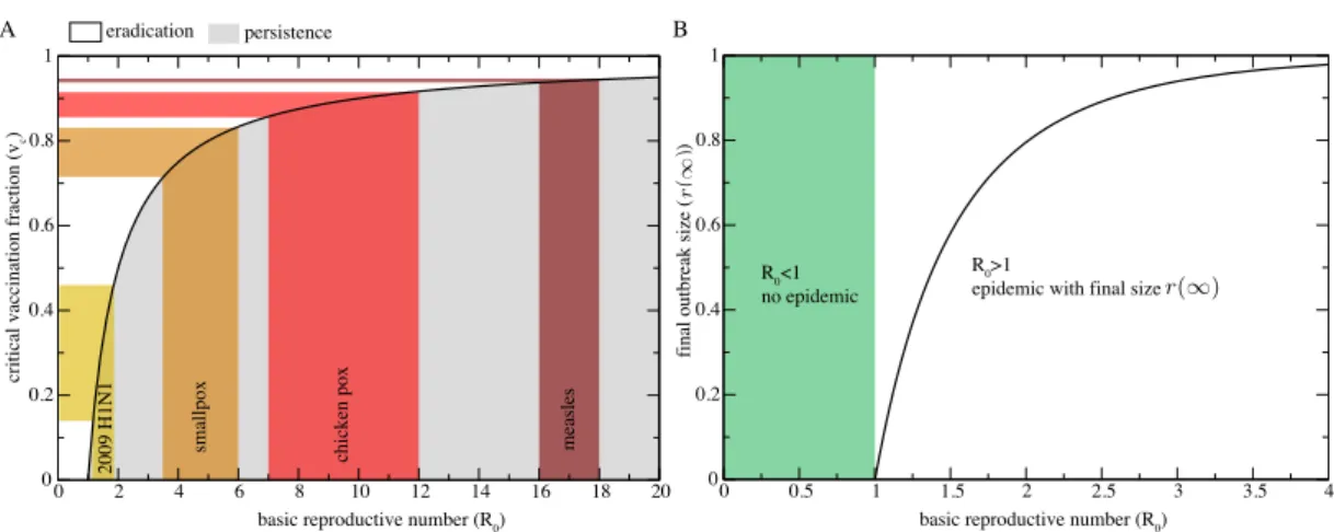
Figure 3.1: (A) Eradication Criterion. The critical fraction of people that has to be vaccinated
to eradicate the disease as a function of R0 is shown. (B) Final outbreak size as a function of the
basic reproductive number.
number of new secondary cases that an infected individual may infect in a fully susceptible population before getting recovered.
The relevance of the epidemic threshold is also related to the protection of populations by means of immunization programs. These correspond to vaccination policies aimed at the eradication of the epidemics. Let us imagine that a fraction v = V /N of the original population is vaccinated and thus fully immune to the disease. The initially susceptible individuals are s(0) = 1−v −i(0), and the linear approximation is therefore:
di(t)/dt = [µ + β(1− v)]i(t) (3.7) The new condition for observing an epidemic outbreak is R�
0= βµ(1− v) > 1. It is thus possible
to define the critical vaccination fraction vc= 1− µ β = 1− 1 R0 (3.8) representing the fraction of individuals to immunize to eradicate an infection. As shown in Figure 3.1A, because of a herd immunity it is not necessary to vaccinate everyone to eradicate an infection. If the vaccine is not perfect and has an efficacy 0 < E ≤ 1 of preventing the transmission from an infected contact, then vc = E1(1− R10). It may happen that for highly
infectious diseases (large R0) and not so effective vaccines (small E), the critical vaccination
Considering the SIR compartmentalization it is also possible to approximately evaluate the final size of the epidemic (73). Considering the equations 3.4, let us divide the variation of susceptible individuals by the variation of recovered ones:
ds dr =
−βs(t)i(t)
µi(t) =−R0s(t) (3.9)
Integrating with respect to dr, we obtain s(t) = s(0)e−R0r(t). Now, when the epidemic is over,
by definition, we have i(∞) = 0 and s(∞) = 1 − r(∞). We thus end up with the transcendental equation:
r(∞) = 1 − s(0)e−R0r(∞) (3.10)
Ideally, it is possible to estimate the basic reproductive number of a disease using the total number of infected cases using the formula 3.10. In Figure 3.1B the final size is shown as a function of R0.
It is important to stress that the deterministic continuous equations presented here are valid only in case of sufficiently large populations and in general a more realistic approach able to capture the natural chance effects of the epidemic transmission would require a full stochastic description. To account for this variability the stochastic dynamics rely on an integer-based population and events occur at probabilistic rates. The linear analysis of the SIR model high-lights the presence of three basic stages in an epidemic evolution. Initially when few infected individuals are introduced in the population we define a pre-outbreak stage in which the evo-lution is noisy and dominated by stochastic effects that are extremely relevant in the presence of few contagious events. This is a stage in which epidemics may or may not disappear from the population just because of stochastic effects. When the infected individuals are enough to make stochastic effects negligible, but still very few compared with the whole population, we observe an exponential take off of the infected cases as described by the equation 3.5. Finally, the decrease of susceptible individuals reduces the force of infection of each infected individual and the exponential growth cannot be sustained any longer in the population, we observe the epidemic turn over and the outbreak will ultimately disappear. However, it is worth stressing that while the outbreak will occur with finite probability if the parameters poise the system above the epidemic threshold, this probability is not equal to one. Actually the stochastic fluctuations may lead to the extinction of the epidemics even well above the epidemic threshold. It has been shown (72) that the extinction probability of an epidemic starting with I0infected individuals is
equal to R−I0
high as 2 the outbreak probability is just 50%.
3.2
Epidemic spreading on graphs
In the previous section we have presented the simple compartmental epidemic models to inves-tigate an infectious disease spreading in a homogeneous population disregarding every possible substructure (gender, age, risk groups, etc...). As already mention, the parameter β governs in an effective way the transmission rate of the disease between infectious and susceptible individuals. In particular, the approximation adopted so far where the β value has been rescaled in order to disregard the usually unknown average number of contacts �k� through which the disease can be transmitted, is equivalent to consider the spreading on a random graph. Nevertheless, many real social and technological networks of epidemiological relevance (mobility networks, the web of sexual contacts, internet, etc...) are far for being homogeneous and the hypothesis that each individual in the system has the same number of connections k� �k� might not be a good approximation.
In this section, by describing the epidemic spreading on a networked system, we show that the fluctuations play a main role in determining the epidemic properties and the spreading may be favored in heterogeneous networks (27; 71; 77; 78). Let us consider an uncorrelated graph com-pletely defined by the degree distribution P (k), and let us divide the nodes according to their health status. The disease can be transmitted from one node to the other only if the nodes are connected through an edge. In order to take into account the heterogeneity induced by the presence of nodes with different connectivity, here we will use a degree block approximation (77; 79; 80): all nodes with the same degree are statistically equivalent. Thus our results will not apply to structured networks in which a distance or a time ordering can be defined; for instance, when the small-world property is not present (79; 81). Here, we have to relax the homogeneous mixing hypothesis made in the previous section and leading to equation 3.4 and work instead with the relative density of infected and susceptible vertices with given degree k:
ik= Ik Nk , sk= Sk Nk . (3.11)
and the global averages are given by: i =� k P (k)ik , s = � k P (k)sk. (3.12)
Let us first consider the very simple SI model. In this case we know that the whole connected component of the system will be infected independently of the spreading rate, but it is very interesting to see the effect of topological fluctuations on the spreading velocity. Considering the class of degree k and defining θk(t) the density of infected neighbors of vertices of degree k the
evolution equations read:
dtik(t) = β[1− ik(t)]kθk(t). (3.13)
The term θk represents the average probability that any given neighbor of a node of degree
k is infected, in the homogeneous assumption it is equal to the density of infected nodes. By considering that at least one of the edges of each infected vertex points to another infected vertex from which the infection has been transmitted, the most general expression for θk is
θk=
�
k�
k�− 1
k� P (k�|k)ik�. (3.14)
The simplest case we can analyze is a network with no degree correlations meaning that the probability that an edge departing from a vertex of degree k arrives at a vertex of degree k� is
independent from the degree of the initial vertex k. In this case the conditional probability does not depend on the originating node and it is possible to show that P (k�|k) = k�P (k�)/�k� and
thus
θk(t) = θ(t) =
�
k�(k�− 1)P (k�)ik�(t)
�k� . (3.15)
Using this in 3.13 and neglecting the terms i2, we have:
dtik(t) = βkθ(t), (3.16)
multiplying both sides of this expression by (k− 1)P (k) and summing over k we get: dtθ(t) = βθ(t) � �k2� �k� − 1 � . (3.17)
We can solve these equations fixing ik(t = 0) = i0 getting:
ik(t) = i0 � 1 + k(�k� − 1) �k2� − �k�(e t/τ− 1) � , (3.18) with τ = �k� β(�k2� − �k�). (3.19)
It is clear that the fraction of infected individuals increases exponentially. This process is faster for high degree nodes. The growth time scale is measured by the heterogeneity ratio�k2�/�k�. For
in the limit N → ∞ we have an unbounded second moment, then in uncorrelated scale-free networks we would have a virtually instantaneous rise of the epidemic size. The reason for that is quite intuitive. Once the disease has reached the hubs it can spread rapidly among the network. Multiplying both sides by P (k) and summing over all k we get:
i(t) = i0 � 1 +�k� 2− �k� �k2� − �k�(e t/τ − 1) � . (3.20)
The above results can be easily extended to the SIR model. Here the variation of infected individuals of degree k has to take into account also the recovery process:
dtik(t) = βksk(t)θk(t)− µik(t), (3.21)
where sk(t) = 1− rk(t)− ik(t). Again considering the linear approximation and uncorrelated
networks we get the time scale τ :
τ = �k�
β�k2� − (µ + β)�k�. (3.22)
The fluctuations are again very important, and here they play a crucial role in the definition of the epidemic threshold. In order to ensure an epidemic outbreak the condition τ > 0 must be satisfied:
β µ≥
�k�
�k2� − �k�. (3.23)
For scale-free networks with exponent 2 < γ≤ 3 in the limit of infinite size the second moment diverges, so we have a null epidemic threshold. This is an important result that confirms how heterogeneous networks behave in a completely different way from homogeneous networks. Scale-free networks are then an ideal topology for the spreading of infectious diseases.
3.3
Metapopulation models
In the previous section we studied systems with a homogeneous mixing approximation or struc-tured populations in which each node of the network corresponds to a single individual. Recently the effect of heterogeneous connectivity patterns has been studied in the case in which each node of the system may be occupied by any number of particles and the connections allow for the displacement of particles form one node to the other (82). In an epidemic framework, particles represent hosts moving between different locations, such as cities or urban areas called, in general, subpopulations. These models are called metapopulations epidemic models and can be formal-ized on different theoretical substructures, from regular lattices to random graphs, but in the last
population i
population j i
j
Subpopulation Individuals health status
Susceptible Infected Recovered host mobility
Metapopulation
Figure 3.2: Representation of a metapopulation model. Each node of the system contains a population of individuals who are characterized with respect to their stage of the disease. In this case we are considering Susceptible, Infected and Recovered indicated in different colors in the picture. Individuals can diffuse from a subpopulation/node to another on the network of connections among subpopulations.
years the abundance of data-driven networks which trace the activities of individuals have led to models based on the detailed knowledge of the spatial structure of the environment and of trans-portation infrastructures, movement patterns and traffic networks (78; 83; 84; 85; 86; 87; 88). In this framework, the nodes of the network are the subpopulations and the coupling among them is shaped by the connectivity patterns represented by the network topology resulting by the movement of individuals from one subpopulation to the other. A sketch of the metapopu-lation approach is shown in Figure 3.2. Each node i is connected to other ki nodes according
to its degree resulting in a network with degree distribution P (k) and distribution moments �kα� =�
kkαP (k).
Realistic descriptions are provided by explicit mechanistic approaches, in which detailed rates of traveling/commuting obtained from data, or from empirical fit to gravity law models, are included (78; 89). A typical assumption is to consider the diffusion process as Markovian implying that the movements of individuals have no memory. Individuals are not labeled according to their original subpopulation, so they move without having memory of their origin. At each time step the movement of individuals is given according to a matrix pijthat encodes the probability that
an individual in the subpopulation i will travel to the subpopulation j. Being wij the traffic
among subpopulations and Ni the number of individuals living in the node i, we define
pij ∼
wij
Ni
These probabilities in realistic models are obtained from real data (45; 78; 90; 91; 92; 93; 94; 95; 96).
Individuals in the same location may get in contact and interact according to the infection dynamics modeled as a reaction process. Within each subpopulation they are divided into classes denoting their health status according to the modeled disease (71). A key point is to evaluate the force of infection generated by the infectious individuals in subpopulation j on the individuals in subpopulation i (84; 85; 97; 98; 99; 100). In the case of a simple SIR model for the evolution of the disease, the metapopulation approach amounts to writing, for each subpopulation, equations such as:
∆Ii(t) = f (Ii, Si, Ri) + Ωi(I) (3.25)
where the first term represents the variation of infected individuals due to the infection dynamics within the subpopulation i and the second term corresponds to the net balance of infectious individuals traveling in and out of the city i. This last term, the transport operator Ωi, depends
on the probability pijthat an infected individual will go from city i to city j and can be generally
written as:
Ωi(I) =
�
i
(pjiIj− pijIi) (3.26)
representing the total sum of infectious individuals arriving in subpopulation i from all connected subpopulations j, minus the amount of individuals traveling in the opposite directions. Similar equations can be written for all the compartments included in the disease model, finally leading to a set of equations where the transport operator acts as a coupling term among the evolution of the epidemics in the various subpopulations.
3.4
Conclusion
We are aware that the transmission of airborne diseases is influenced by many biological, social and environmental factors. For instance, the infectivity of a diseased individual depends on the viral load (101; 102) as well as the susceptibility is influenced by the individual antibody response. The age-specific contact patterns (103; 104) have been found to be relevant for infections trans-mitted by the respiratory or close-contact route and, finally, it has been recognized that the ab-solute air humidity may contribute to disseminate viruses in aerosolized droplets (105; 106; 107). Nevertheless, with the basic compartmental description introduced in this chapter, where all these factors are disregarded or flattened out, it is possible to achieve important insights about an infectious disease spreading. Such approach represent the first step in the epidemic modeling,
and we discussed how through the homogeneous mixing approximation it is possible to derive a mathematical description of the epidemic threshold, the final size of an epidemic outbreak and the critical vaccination fraction. We then briefly described how the modeling of disease spread-ing on networked settspread-ings can take advantage of the degree-block approximation in order to take into account the heterogeneity of the system due to different contact patterns. This approach will be crucial in chapter 5 for the analytical assessment of the disease containment by means of human mobility restrictions. Furthermore, in chapter 6, leveraging on a network description, we will present a systematic investigation of an emerging infectious disease spreading through the Italian livestock premises. Finally, the metapopulation framework introduced in the last section represents the starting point for presenting the Global Epidemic and Mobility (GLEaM) model described in chapter 4 and chapter 5.
GLobal Epidemic and Mobility
model
Contents
4.1 Global Population and subpopulations definition . . . 30
4.2 World Airport Network . . . 32
4.3 Commuting Networks . . . 32
4.4 Epidemic model . . . 35
4.5 Stochastic and discrete integration of the disease dynamics . . . . 36
4.6 The integration of the transport operator . . . 37
4.7 Time-scale separation and the integration of the commuting flows 38
4.8 Effective force of infection . . . 40
In this chapter we present in detail the Global Epidemic and Mobility model (GLEaM), that is a discrete stochastic epidemic computational model based on a meta-population approach able to perform numerical simulations of global epidemic spreading. The design and implementation of GLEaM started in 2005 and in the last years it involved almost twenty collaborators from different laboratories in Europe and the US. Along with the academic research, the GLEaMviz project (www.gleamviz.org) is devoted to provide a public software with a user friendly inter-face for the simulation of large-scale epidemic outbreaks and to participate to outreach activities about emerging infectious diseases spreading. During my PhD training, within the Computa-tional Epidemiology Laboratory at the I.S.I. Foundation, Turin, IT, I have contributed to the development of GLEaM by collecting and analyzing part of the short range mobility data
in-cluded in the model, and by testing and implementing the computational infrastructure described in this chapter. GLEaM is coded in C/C++ and runs conveniently on high-end desktop ma-chines. The results presented in chapter 5 were achieved by using GLEaM to investigate the H1N1 2009 influenza pandemic. In this context, I have performed part of the simulations for the estimation of the disease parameters as described in 5.2 and I have performed the numerical estimate of the number of cases in Mexico in the early phase of the outbreak as discussed in 5.4. I have implemented the code, performed the simulations and analyzed the results to test different intervention strategies as described in sections 5.5.1 and 5.5.3 and I have helped in the analysis and the assessment of the critical care demand presented in 5.5.2. Furthermore I have performed the simulations and provided the data for the implementation of the “Epidemic Planet” scientific exhibit (http://www.gleamviz.org/outreach-activities/) that was hosted at the International Science Festival that took place in Edinburgh, UK, April 3 - 17, 2010 and at the International Conference for High Performance Computing, Networking, Storage and Anal-ysis that took place in New Orleans, LA, USA, November 13 - 19, 2010
Structured metapopulation model
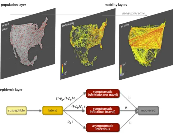
Here we present the detailed definition and data description of the global structured metapopu-lation model. The computational model is based on three data/model layers. The first layer is a data layer defining the census area and the subpopulation structure. The second one refers to human mobility model defined by the transportation and commuting networks characterizing the interactions and exchanges of individuals across subpopulations. The third layer is the epidemic dynamic model that defines the evolution of the infectious disease inside each subpopulations.
4.1
Global Population and subpopulations definition
The population dataset was obtained from the Web sites of the ”Gridded Population of the World” and the ”Global Urban-Rural Mapping” projects (108; 109), which are run by the Socioeconomic Data and Application Center (SEDAC) of Columbia University. The surface of the world is divided into a grid of cells that can have different resolution levels. Each of these cells has assigned an estimated population value.
Out of the possible resolutions, we have opted for cells of 15× 15 minutes of arc to constitute the basis of our model. This corresponds to an area of each cell approximately equivalent to a