HAL Id: hal-03210805
https://hal.archives-ouvertes.fr/hal-03210805v2
Submitted on 5 Jul 2021
HAL is a multi-disciplinary open access
archive for the deposit and dissemination of
sci-entific research documents, whether they are
pub-lished or not. The documents may come from
teaching and research institutions in France or
abroad, or from public or private research centers.
L’archive ouverte pluridisciplinaire HAL, est
destinée au dépôt et à la diffusion de documents
scientifiques de niveau recherche, publiés ou non,
émanant des établissements d’enseignement et de
recherche français ou étrangers, des laboratoires
publics ou privés.
Distributed under a Creative Commons Attribution| 4.0 International License
Loïc Paulevé, Sylvain Sené
To cite this version:
Loïc Paulevé, Sylvain Sené. Non-deterministic updates of Boolean networks. 27th IFIP WG 1.5
International Workshop on Cellular Automata and Discrete Complex Systems (AUTOMATA 2021),
2021, Marseille, France. pp.10:1–10:16, �10.4230/OASIcs.AUTOMATA.2021.10�. �hal-03210805v2�
Loïc Paulevé
# ÑUniversité Bordeaux, Bordeaux INP, CNRS, LaBRI, UMR5800, F-33400 Talence, France
Sylvain Sené
# ÑUniversité Publique, Marseille, France
Abstract
Boolean networks are discrete dynamical systems where each automaton has its own Boolean function for computing its state according to the configuration of the network. The updating mode then determines how the configuration of the network evolves over time. Many of updating modes from the literature, including synchronous and asynchronous modes, can be defined as the composition of elementary deterministic configuration updates, i.e., by functions mapping configurations of the network. Nevertheless, alternative dynamics have been introduced using ad-hoc auxiliary objects, such as that resulting from binary projections of Memory Boolean networks, or that resulting from additional pseudo-states for Most Permissive Boolean networks. One may wonder whether these latter dynamics can still be classified as updating modes of finite Boolean networks, or belong to a different class of dynamical systems. In this paper, we study the extension of updating modes to the composition of non-deterministic updates, i.e., mapping sets of finite configurations. We show that the above dynamics can be expressed in this framework, enabling a better understanding of them as updating modes of Boolean networks. More generally, we argue that non-deterministic updates pave the way to a unifying framework for expressing complex updating modes, some of them enabling transitions that cannot be computed with elementary and non-elementary deterministic updates.
2012 ACM Subject Classification Theory of computation → Models of computation; Theory of computation → Program semantics; Applied computing → Systems biology
Keywords and phrases Natural computing, discrete dynamical systems, semantics
Digital Object Identifier 10.4230/OASIcs.AUTOMATA.2021.10
Funding Loïc Paulevé: French Agence Nationale pour la Recherche (ANR): ANR-FNR project “AlgoReCell” ANR-16-CE12-0034 and ANR project “BNeDiction” ANR-20-CE45-0001.
Sylvain Sené: his salary as a French state agent affiliated to Université Aix-Marseille, Université Toulon, CNRS, LIS, UMR 7020, Marseille, France, and the ANR project “FANs” ANR-18-CE40-0002.
1
Introduction
Boolean networks (BNs) are formal dynamical systems composed of automata, each of them having a Boolean state. A major difference between BNs and cellular automata (CAs) is that each automaton of a BN follows its own rules for computing its next state depending on the states of the other automata in the network. Consequently, whereas influences between cells in a CA are structured homogeneously according to a cellular space, those between automata in a BN are structured according to any directed graph. In this paper, only finite BNs are considered, as it is generally the case in the literature, notably because BNs are mostly viewed as both a real-world computational model and a real-world modeling framework.
The study of BNs led to fundamental results linking the network architecture (structure of influences between automata) to the existence of fixed points and to the number of limit cycles they can exhibit [1, 10, 4]. Notably, it is well known that such limit behaviors may depend on the way automata update their state over time [3, 12, 2, 22]. This emphasizes the importance of what is classically called the updating modes in the analyses of BNs.
© Loïc Paulevé and Sylvain Sené;
licensed under Creative Commons License CC-BY 4.0
27th IFIP WG 1.5 International Workshop on Cellular Automata and Discrete Complex Systems (AUTOMATA 2021).
Editors: Alonso Castillo-Ramirez, Pierre Guillon, and Kévin Perrot; Article No. 10; pp. 10:1–10:16 OpenAccess Series in Informatics
BNs are widely employed to model natural systems, with prominent applications in biology. These applications inspired the definition of various updating modes aiming at reflecting constraints related to the quantitative nature of the abstracted system, such as reaction duration and influence thresholds. There is actually no consensus about one updating mode that would be the most likely, the most representative of the biological reality. As a consequence, the choice of this or that updating mode strongly depends on the problematics, on the nature of the questions addressed. Thus, it remains essential to analyze the impact of a wide range of updating modes with distinct features.
In this paper, we address the formalization of updating modes in the framework of BNs. From a very general perspective, given a BN and one of its configurations, an updating mode specify how to compute the possible next configurations (plural implying non-deterministic systems).
A large majority of updating modes introduced so far can be expressed using deterministic functions mapping the configurations of the network. This leads to elementary transitions, as it is the case with synchronous (or parallel) and asynchronous [23] updating modes, which may result in non-deterministic dynamics. These functions may also be composed, as in block-sequential [25] and block-parallel [11] updating modes, generating non-elementary transitions.
These compositions of deterministic updates, however, do not cover all the updating modes introduced in the literature. Indeed, updating modes may also make use of parameters that cannot a priori and intuitively be directly captured by these deterministic updates. These parameters can represent kinds of delays or threshold effects of state changes. In this paper, we focus on 3 examples of BN dynamics which have been recently introduced and defined using ad-hoc formalizations:
Memory Boolean networks (MBNs) [14, 15] take into account some kind of delay for the decrease of automata. They have been introduced by the means of a deterministic dynam-ical system with non-binary configurations, whose updates are computed deterministdynam-ically from the BN and a memory vector, specifying the delay for each automaton.
Interval Boolean networks (IBNs) [7] account for a duration for updating an automaton. The other automata can be updated until the former automaton eventually change of state. They have been defined by an encoding as the fully-asynchronous updating of a BN of dimension 2n. The dynamics of the original BN are then recovered by projection. Most Permissive Boolean networks (MPBNs) [24] bring a formal abstraction of trajectories of quantitative models which are compatible with the BN formalism: from an initial configuration, if there is no trajectory where a given automaton is 1 (or 0), then, no quantitative refinement of the model can increase (or decrease) the value of this automaton. MPBNs have been defined by introducing additional states for automata to account for their state change (increasing and decreasing). An automaton in one of these states can be read non-deterministically as 0 or 1.
Overall, the definition of these BN dynamics involve either non-Boolean configurations, projections of higher-dimension BN, or both. Importantly, they suggest that deterministic updates are not expressive enough to capture specific dynamics. This is striking with IBNs and MPBNs which can generate transitions that are neither elementary nor non-elementary transitions, and thus predict trajectories that are impossible with the asynchronous updating mode.
We show that these dynamics can all be expressed using Boolean configurations in a simple generic framework, which extends the deterministic updates to non-deterministic updates: functions mapping sets of configurations. In the case of MBNs, the obtained
definition from the binary projections of their deterministic discrete dynamics actually help to understand the generated dynamics: the transitions match with a particular subset of elementary transitions, suggesting a simpler parameterization. In the case of IBNs and MPBNs, the transitions extend the elementary and non-elementary transitions by considering some delay for the state changes, and having different interpretation of how to “read” an automaton in the course of state change. The obtained definitions suggest many variants for generating sub-dynamics, similarly to the asynchronous mode which generates all elementary transitions.
Thus, non-deterministic updates offer a unified yet simple framework for defining and understanding BN updating modes with more expressivity than usual deterministic updates. However, should any set update be considered as a BN updating mode? We propose an argumentation for a reasonable updating mode in the last section, where we suggest that the state change should always be justified by the application of a local function. This suggests that the MP updating mode generates the largest set of transitions that fulfill this criterion. Notations. The Boolean domain {0, 1} is denoted by B; the set {1, · · · , n} is denoted by JnK. Given a finite domain A with a partial order ⪯, and a function h mapping elements of A to A, for any k ∈ N>0, we write hk for h iterated k times. Whenever for any a ∈ A,
a ⪯ h(a), we write hω for the iteration of h until reaching a fixed point (in this paper, A is
often a power set with ⪯ being the subset relation).
2
Boolean networks and dynamics
A Boolean network (BN) of dimension n is specified by a function f : Bn → Bn mapping
Boolean vectors of dimension n. The componentsJnK of the BN are called automata. For each automaton i ∈JnK, fi: Bn→ B is the i-th component of this function, that we call the
local function of automaton i. The 2n Boolean vectors of Bn are called the configurations of the BN. In a configuration x ∈ Bn, x
i is the state of automaton i.
Updating modes. Given a BN f of dimension n and one of its configurations x ∈ Bn, an updating mode µ characterizes the possible evolutions of x with respect to f (x). The dynamical system (f, µ) defines a binary transition relation between configurations of Bn denoted by −→(f,µ)⊆ Bn× Bn. This dynamical system can be represented by a directed
graphD(f,µ)= (Bn, −→(f,µ)). This graph is usually called the transition graph of (f, µ). The
reflexive and transitive closure of relation −→(f,µ), denoted by −→∗(f,µ)can be defined as follows:
given two configurations x, y ∈ Bn, x −→∗
(f,µ)y if and only if x = y or there exists a path
from x to y inD(f,µ).
A deterministic updating mode ensures that, for any BN f of dimension n, each configur-ation has at most one outgoing transition (∀x, y, z ∈ Bn, x −→
(f,µ)y and x −→(f,µ)z only if
y = z). Otherwise, the updating mode is qualified as non-deterministic.
In the following, we consider the BN f to be fixed, and thus, for the sake of simplicity, we omit the subscript f : the transition relation is denoted by −→µ and the transition graph
byDµ.
Dynamical properties. A configuration x ∈ Bn is transient if there exists a configuration
y such that x −→∗
µ y and y ̸−→∗µ x. Configurations that are not transient are called limit
configurations. Because n is finite, these configurations induce the terminal strongly connected components ofDµ, called the limit sets of (f, µ). If there exists at least one path from a
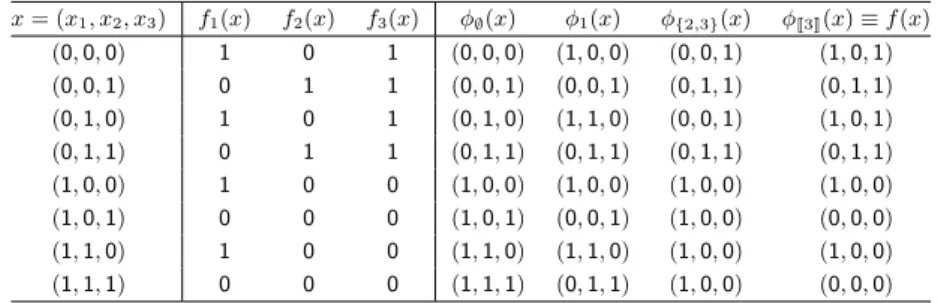
Table 1 Configurations, local functions ((fi)i∈
J3K) and four updating functions (ϕ∅, ϕ1, ϕ{2,3},
and ϕJ3K) of Boolean network f presented in Example 2.
x = (x1, x2, x3) f1(x) f2(x) f3(x) ϕ∅(x) ϕ1(x) ϕ{2,3}(x) ϕJ3K(x) ≡ f (x) (0, 0, 0) 1 0 1 (0, 0, 0) (1, 0, 0) (0, 0, 1) (1, 0, 1) (0, 0, 1) 0 1 1 (0, 0, 1) (0, 0, 1) (0, 1, 1) (0, 1, 1) (0, 1, 0) 1 0 1 (0, 1, 0) (1, 1, 0) (0, 0, 1) (1, 0, 1) (0, 1, 1) 0 1 1 (0, 1, 1) (0, 1, 1) (0, 1, 1) (0, 1, 1) (1, 0, 0) 1 0 0 (1, 0, 0) (1, 0, 0) (1, 0, 0) (1, 0, 0) (1, 0, 1) 0 0 0 (1, 0, 1) (0, 0, 1) (1, 0, 0) (0, 0, 0) (1, 1, 0) 1 0 0 (1, 1, 0) (1, 1, 0) (1, 0, 0) (1, 0, 0) (1, 1, 1) 0 0 0 (1, 1, 1) (0, 1, 1) (1, 0, 0) (0, 0, 0)
transient configuration to a limit set, this limit set is called an attractor of (f, µ) [8, 21]. The basin of attraction of an attractor A of (f, µ), denoted by B(A), is the sub-graph of Dµ induced by the set of transient configurations x such that, for any limit configuration
y belonging to A, x −→∗
µ y. A limit set of cardinal 1, i.e. composed of a unique limit
configuration x is called a fixed point of (f, µ). A limit set of cardinal greater than 1 is called a limit cycle of (f, µ).
3
Updating modes with deterministic updates
Elementary transitions
Let us consider a BN f of dimension n and one of its configurations x ∈ Bn. Whenever x and
f (x) differ by more than one component, one may define several ways to update x: either by replacing it with f (x), i.e., applying simultaneously the local functions on every automata, or by modifying the state of only a subset of automata. For each set of automata to update, we obtain a deterministic function mapping configurations, that we refer to as an elementary deterministic update:
▶Definition 1. Given a BN f of dimension n and a set of automata W ⊆JnK, ϕW : B
n
→ Bn
is an elementary deterministic update with
∀x ∈ Bn, ∀i ∈
JnK, ϕW(x)i= (
fi(x) if i ∈ W ,
xi otherwise.
Whenever referring to singleton sets {i} with i ∈JnK, we write ϕi instead of ϕ{i}. Notice
that ϕ
JnK= f .
▶ Example 2. Let us consider the BN f of dimension n = 3 with f (x) = f1(x) = ¬x3 f2(x) = ¬x1∧ x3 f3(x) = ¬x1 .
Table 1 shows four distinct updatings on its configurations. The first updating is ineffective and consists in changing nothing. The second updating changes the state of automaton 1 by application of ϕ1, the third one changes the states of both automata 2 and 3 by application
of ϕ{2,3}, and the fourth one changes the state of every automaton by application of ϕJ3K.
We can then define the notion of elementary transitions of a BN, that are the transitions obtained by applying any elementary update on a non-empty subset of automata.
000 001 010 011 100 101 110 111 000 001 010 011 100 101 110 111 000 001 010 011 100 101 110 111
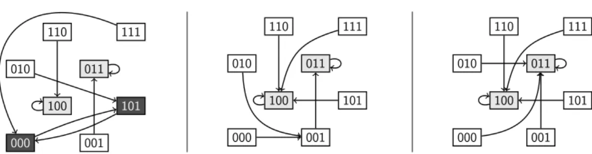
Figure 1 Distinct possible block-sequential dynamics of BN f defined in Example 2: (left panel) its parallel dynamics associated with ordered partition (J3K); (central panel) the block-sequential dynamics associated with ({2, 3}, {1}); (right panel) the block-sequential dynamics associated with ({3}, {1}, {2}).
▶Definition 3. Given a BN f , its elementary transitions −→e ⊆ Bn× Bn are such that,
for all configurations x, y ∈ Bn, x −→e y if and only if there exists a non-empty subset of
automata W ⊆JnK with y = ϕW(x).
Let us now define some classical deterministic and non-deterministic updating modes from these elementary updates.
Examples of deterministic updating modes
The most direct updating mode is the application of f to the configuration x, resulting in the configuration f (x), or, equivalently, ϕ
JnK(x):
▶Definition 4. The synchronous (or parallel) updating mode of a BN f of dimension n generates the transition relation →p ⊆ Bn× Bn such that, for all configurations x, y ∈ Bn,
x →py if and only if y = ϕJnK(x).
Sequential updating modes are parameterized by a permutation ofJnK, fixing an ordering of elementary updates of single automata [13, 17, 9]. They can be generalized to block-sequential updating modes [25, 3, 16], parameterized by a permutation of a partition ofJnK:
▶Definition 5. Given a BN f of dimension n and bs = (W1, · · · , Wp) an ordered partition
ofJnK, the block-sequential updating mode generates the transition relation →bs ⊆ Bn× Bn
such that, for all configurations x, y ∈ Bn, x →bsy if and only if y = ϕWp◦ · · · ϕW1(x).
Remark that the transitions of sequential and block-sequential modes may not be ele-mentary. However, they always correspond to a path of elementary transitions: x →bsy only
if x →∗e y.
Going further in generalization, one may consider deterministic updating modes as infinite sequences of sets of automata, so that automata of a same subset execute their local function in parallel while the subsets are iterated sequentially. Remark that any of these possible deterministic updating modes will generate transitions corresponding to specific paths of elementary transitions.
Examples of non-deterministic updating modes
It is important to notice that deterministic updates can lead to non-deterministic dynamics by allowing different updates on a same configuration. The most obvious example is the asynchronous mode1 consisting of all the elementary transitions.
1 The asynchronous mode is often referred to as general asynchronous in the systems biology modeling
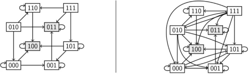
000 001 010 011 100 101 110 111 000 001 010 011 100 101 110 111
Figure 2 Fully-asynchronous (left) and asynchronous (right) dynamics of BN f defined in Example 2.
▶Definition 6. The asynchronous updating mode of a BN f generates the transition relation →a ⊆ Bn× Bn as →a= →e.
One of the most usual non-deterministic updating modes of BNs is the fully-asynchronous mode2, where only one automaton is updated in a transition. It is largely employed for the analysis of models of biological systems, arguing it enables capturing (some) behaviors caused by different time scale for automata updates.
▶Definition 7. The fully-asynchronous updating mode of a BN f generates the transition relation →fa ⊆ Bn× Bn such that, for all configurations x, y ∈ Bn: x →fay if and only if
there exists i ∈JnK with y = ϕi(x).
Figure 2 shows the dynamics generated by the fully-asynchronous and asynchronous updating modes on the BN of Example 2.
4
Non-deterministic updates as set updates
The updates considered so far are deterministic, and can thus be defined as functions mapping configurations, i.e., of the form ϕ : Bn→ Bn. As we have seen above, deterministic updates
can generate non-deterministic updating modes, by allowing different updates to be applied on a same configuration.
Let us now extend to non-deterministic updates, that we model by functions mapping sets of configurations, i.e., of the form Φ : 2Bn → 2Bn. We define Φ as a map from sets
of configurations to sets of configurations for enabling iterations and compositions of non-deterministic updates. Nevertheless, we assume that for any X ⊆ Bn, Φ(X) =S
x∈XΦ({x}):
one can define Φ only from all singleton configuration set. This restriction ensures that, for any X ⊆ Bn, each configuration in the image set y ∈ Φ(X) can be computed from a singleton
set {x} for some x ∈ Bn. In the following, we call such updates set updates.
Starting from a singleton configuration set {x}, the iteration of set updates delineates the domains of configurations the system can evolve to. Thus, set updates naturally define transition relations between configurations:
▶ Definition 8. Given a set update function Φ for BNs of dimension n, the generated transition relation is given by δ : (2Bn → 2Bn) → 2Bn×Bn
with δ(Φ) = {(x, y) | x ∈ Bn, y ∈ Φ({x})}.
2 The fully-asynchronous mode is usually referred to as asynchronous in the system biology modeling
In contrast with deterministic updates, non-deterministic updating modes can be charac-terized directly by set updates. Indeed, non-deterministic updating modes allow “superposing” alternative updates to generate different transitions from a single configuration x, although each of them is computed with a deterministic update. For instance, with one update ϕ where ϕ(x) = y and another update ϕ′ where ϕ′(x) = y′ ̸= y. Now, let us imagine an updating mode superposing two set updates, Φ and Φ′ where, for some configurations x ∈ Bn, Φ({x}) \ Φ′({x}) ̸= ∅. One can then build a single set update Φ∗ such that
Φ∗(X) = Φ(X) ∪ Φ′(X). It results that δ(Φ∗) = δ(Φ) ∪ δ(Φ′), thus the updating mode can be assimilated to Φ∗.
Finally, notice that limit sets of the generated dynamics δ(Φ) can be characterized as the ⊆-smallest sets of configurations X ⊆ Bn such that Φ(X) = X.
5
Updating modes selecting elementary transitions
With deterministic updates as building blocks, we have seen that one can define non-deterministic updating modes by superposing different update functions. The resulting transition relation is then the union of the transition relation generated by each individual update (each of them giving a deterministic dynamics). Set updates offer an alternative way to formalize the resulting dynamics, by directly defining the set of out-going transitions from a given configuration. As we will illustrate with the memory updating mode below, this enables a fine-grained selection of the elementary transitions which may then depend on the configuration.
5.1
Asynchronous and fully-asynchronous updating modes
As a first illustration of set updates and how they can characterize updating modes, consider the following set update for BNs of dimension n:
Φe(X) = {ϕW(x) | x ∈ X, ∅ ̸= W ⊆JnK}.
This set update generates exactly all the elementary transitions: δ(Φe) = →e. Thus, Φe
characterizes the asynchronous updating mode. Similarly, let us now consider the following set update:
Φfa(X) = {ϕi(x) | x ∈ X, i ∈JnK}.
Remark that δ(Φfa) =→fa, i.e., Φfa characterizes the fully-asynchronous updating mode.
5.2
Memory updating mode
Until now, all the updating modes that have been discussed depend on deterministic updates that are context free, which leads to deal with memoryless dynamical systems. In [14, 15] have been introduced another model of BNs, called Memory Boolean networks (MBNs). The first objective of MBNs is to capture the biologically relevant gene-protein BN model introduced in [18], that builds on the following principles:
automata are split in two types: a half models genes, the other half models their associated one-to-one proteins;
each protein has its own decay time: the number of time steps during which it remains present in the cell after having been produced by the punctual expression of its associated gene.
In their original definition given below, MBNs of dimension n are BNs of dimension n parameterized with a vector M ∈ Nn
>0, setting the maximal delay (called memory) for
the degradation of each automaton. Then, an automaton is considered active (Boolean 1) whenever its delay to degradation is not 0. Formally, MBN are defined as follows:
▶Definition 9. A Memory Boolean network of dimension n is the couple of a BN f of dimension n and of a memory vector M = (M1, . . . , Mn) ∈ Nn>0. The set of its configurations
is defined as X(f,M)= {(x, d) ∈ Bn× Nn | ∀i ∈JnK, di ∈ {0, . . . , Mi}, xi = 0 ⇐⇒ di = 0 and xi= 1 ⇐⇒ di ∈ {1, . . . , Mi}}. The dynamical system ((f, M), p) is defined by the
transition graph D((f,M),p), with p the parallel updating mode, made of transitions based on
updating function ϕ⋆: X(f,M)→ X(f,M) depending on the memories such that:
∀(x, d), (y, d′) ∈ X(f,M), (x, d) −→((f,M),p)(y, d′) ⇐⇒ (y, d′) = ϕ⋆ JnK (x, d), where ∀i ∈JnK, ϕ⋆ JnK (x, d)i= (yi, d′i), with: d′i= 0 if fi(x) = 0 and di= 0, di− 1 if fi(x) = 0 and di≥ 1, Mi if fi(x) = 1, and yi= ( 1 if d′i≥ 1, fi(x) if d′i= 0.
From this initial definition, it is easy to see that the dynamics of a MBN is deterministic and operates on discrete configurations that are not Boolean anymore. But we will see that MBNs enable to develop a new updating mode, called the memory updating mode, that operates directly on Boolean configurations.
First, let us define α(x) the set of memory configurations corresponding to any binary configuration x ∈ Bn, and conversely, β(d) the binary configuration corresponding to a memory configuration d ∈ Nn
. Notice that ∀x ∈ Bn, ∀d ∈ α(x), β(d) = x.
α(x) = {d ∈ Nn| xi= 0 ⇔ di= 0, xi= 1 ⇔ di∈JMiK}, ∀i ∈JnK β(d)i= min{di, 1}.
It appears that X(f,M)= {(β(d), d) | d ∈ Nn, ∀i ∈JnK, di ∈ {0, . . . , Mi}}. Thus one can reformulate the original definition by considering the deterministic parallel update of memory configurations d ∈ Nn, and replacing x with β(d): an automaton i ∈JnK is set to state Mi whenever its local function fi is evaluated to 1 on the corresponding binary configuration
β(d); otherwise, its state is decreased by one, unless it is already 0. In particular, one can define the deterministic memory update ϕ∗M: Nn→ Nn such that, for each i ∈
JnK, ϕ∗M(d)i= 0 if fi(β(d)) = 0 and di= 0, di− 1 if fi(β(d)) = 0 and di≥ 0, Mi if fi(β(d)) = 1.
Let us now extend the above definitions to sets: ∀X ⊆ Bn, A(X) =S x∈Xα(x); ∀D ⊆ Nn, B(D) = {β(d) | d ∈ D}; ∀D ⊆ Nn, Φ∗ M(D) = {ϕ ∗ M(d) | d ∈ D}.
The memory set update can then be defined for any set of configurations X ⊆ Bn by first
generating the set of corresponding memory configurations, then applying the deterministic update on them, and finally converting them back to binary configurations:
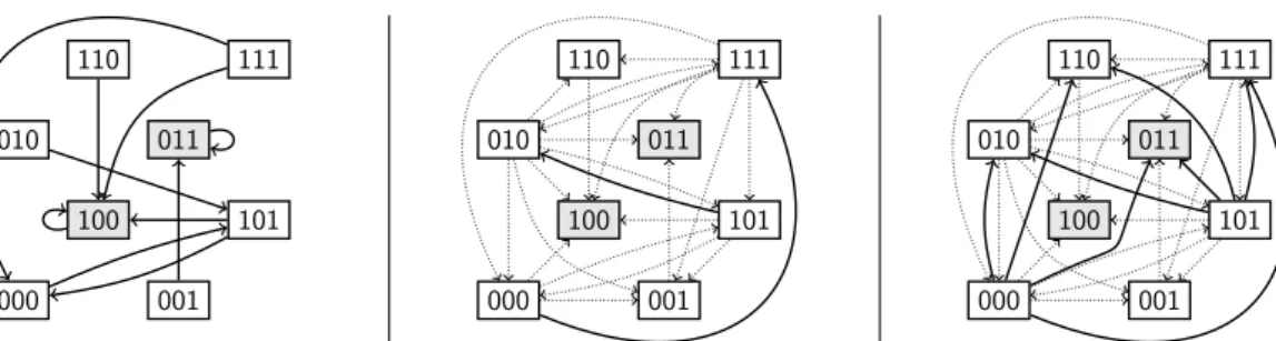
000 001 010 011 100 101 110 111 000 001 010 011 100 101 110 111 000 001 010 011 100 101 110 111
Figure 3 Memory dynamics with M = {1} (left), interval dynamics (center), and MP dynamics (right) of the BN of Example 2. In these two latter, the elementary transitions are dotted and loops
are omitted.
With this formulation, one can see that the memory updating mode, being the projection of MBN configurations on their binary part, lead to non-deterministic dynamics. Indeed, whenever a configuration gets mapped to several possible memory configurations, and whenever for two of these configurations d and d′, there is an automaton i ∈ JnK where ϕM(d)i = 0 and ϕM(d′)i ≥ 1. This can occur if and only if Mi ≥ 2, xi = 1, and fi(x) = 0.
Thus, the memory updating mode of BNs can equivalently be parameterized by a set of automata M = {i ∈JnK | Mi≥ 2} and defined as the following set update:
ΦM(X) = {ϕW(x) | x ∈ X, W ⊆JnK, W ⊇ {i ∈ JnK | i /∈ M ∨ fi(x) = 1}}.
Remark that this definition no longer relies on memory configurations in Nn. Overall, the memory updating mode of BNs can be understood as a particular set of elementary transitions: those where automata not in M or automata that can change from state 0 to 1 are always updated, together with any subset of the others (automata in M that can change from state 1 to 0): automata in M that are decreasing are updated asynchronously, while the others are updated in parallel.
Figure 3(left) gives the dynamics generated by the interval updating mode on the BN of Example 2 with M = {1}.
6
Updating modes going beyond (non-)elementary transitions
BNs are widely used to model dynamics of biological systems, notably implying gene regulation. Gene regulation is a dynamical biological process that involves numerous mechanisms and entities among which some of them, like RNAs and proteins, have specific influences that depend on their concentration. In other terms, the regulation process in its whole admits significant quantitative parts. The question arises then of how faithful are Boolean dynamics with respect to the quantitative dynamics. It has been recently underlined in [24] that the elementary and non-elementary transitions of BNs are not complete enough to capture particular quantitative trajectories. With a fixed logic, and starting from similar configurations, the quantitative system shows that an automaton can eventually get activated, whereas the asynchronous dynamics of the BN shows it is impossible.
In this section, we address the set update reformulation of two recently introduced dynamics of BNs which generate transitions that are neither elementary nor non-elementary: they result in set updates Φ where, for some BNs of dimension n and for some configurations x ∈ Bn, there is k ∈ N such that there exists y ∈ Φk({x}) whereas x ̸→∗e y.
6.1
Interval updating mode
From the concurrency theory, it is known that the execution of 1-bounded contextual Petri nets corresponding to the asynchronous updating mode (known as steps semantics) may miss some transitions that can be triggered when considering certain delay of state change [6, 5]. In [7] is proposed a translation of the interval semantics of Petri nets to BNs, showing it can predict transitions that are neither elementary nor non-elementary transitions: configurations that are not reachable with the asynchronous mode from a fixed initial configuration x become reachable with Interval Boolean networks.
The main principle of the interval dynamics is to decompose the change of state of an automaton, allowing interleaving the update of other automata. For instance, let us assume that automaton i can change from state 0 to 1. In the interval dynamics, we register that i will eventually change to state 1, and then allow the update of other automata, still considering that i is in state 0. In [7], this is applied to any BN of dimension n by an encoding with the fully-asynchronous dynamics of a BN of dimension 2n: each automaton is split in a read and write automaton, where the write automaton register the next state of the original automaton, and the read automaton keeps its current state and will eventually copy the value of the write automaton. The dynamics of the original BN is then obtained by projecting the configurations on the read automata.
We provide below an equivalent formulation as a composition of set updates. Essentially, whenever an automaton i can change its state, we hold it and compute the possible state changes of the automata different than i. Thus, during this evaluation, we have a growing number of held automata, that we denote by L, waiting for their state to be updated. The set update ΦInt,L extends a given set of configurations with the possible state change of
automata not in L. The function Φi/L(x) first computes all possible state changes by iterating
ΦInt,L∪{i}until a fixed point, and then apply the state change for the automaton i on all the
resulting configurations.
▶Definition 10. The Interval set update ΦIntof a BN of dimension n is given by ΦInt= ΦInt,∅
where
ΦInt,L(X) = X ∪ {y ∈ Φi/L(x) | x ∈ X, i ∈JnK, i /∈ L, fi(x) ̸= xi}, Φi/L(x) = {yi| y ∈ ΦωInt,L∪{i}({x})}.
The interval updating mode preserves the fixed points of f : for any configuration x ∈ Bn,
ΦInt({x}) = {x} if and only if f (x) = x. Moreover, one can prove that it includes all the
elementary transitions: for any configuration x ∈ Bn, Φ
e({x}) ⊆ ΦInt({x}).
▶Example 11. Figure 3 shows the transitions generated by the interval updating mode on the BN of Example 2. Notice that there is a path from 000 to 111, which does not exist in the asynchronous dynamics (Figure 2). Indeed, let us partially compute ΦInt,∅({000}) =
{000} ∪ Φ1/∅(000) ∪ Φ3/∅(000).
Let us focus on the interval update of automaton 1 with Φ1/∅(000), which requires
com-puting all the iterations of ΦInt,{1}({000}). The first iteration gives ΦInt,{1}({000}) =
{000} ∪ Φ3/{1}(000) = {000, 001}, then Φ2Int,{1}({000}) = {000, 001} ∪ Φ2/{1}(001) =
{000, 001, 011} = Φω
Int,{1}({000}).
Finally, we get Φ1/∅(000) = {100, 101, 111}. Thus, 111 ∈ ΦInt({000}).
6.2
Most Permissive updating mode
Most Permissive Boolean networks (MPBNs) have been designed to capture all automata updates that could occur in any quantitative refinement of the BN. We will come back more formally to this notion later in this section.
The main feature of MPBNs is to abstract all the possible interaction thresholds between automata. Consider the case whenever the state of an automaton i is used to compute the state of two distinct automata j and k, and assume that i is increasing from 0: during its increase, there are times when i may be high enough for trigger a state change of j but not (yet) high enough for k. This can be illustrated on a concrete biological example, the so-called incoherent feed-forward loop of type 3 [20]: a BN f of dimension 3 with
f1(x) = 1 f2(x) = x1 f3(x) = ¬x1∧ x2.
Starting from the configuration 000, the asynchronous updating mode predicts only the following non-reflexive transitions: 000 →a 100 →a 110. Notice that in this case, the
interval updating mode results in the same transitions. However, it has been observed experimentally [27] and in quantitative models [19, 26] that depending on reaction kinetics, one can actually activate transiently the automata 3. Essentially, the idea is that during the increase of the state of automaton 1, there is period of time where 1 is high enough so 2 can consider it active (x1 true) but 3 still considers it inactive (x1 false). Then, the state of
automaton 2 can increase, and so do the state of automaton 3. This activation of 3 cannot be predicted with BN updating modes defined so far, whereas the logic encoded by f is correct.
Without introducing any parameter, MPBNs capture these additional dynamics by ac-counting for all possible thresholds ordering, for all updates that can happen between a switch of a Boolean state. In some sense, the MP updating mode abstracts both the quantitative domain of automata and the duration of state changes. Their original definition [24] is based on the introduction pseudo dynamic states, namely increasing and decreasing. An automaton can change from 0 to increasing whenever it can interpret the state of the other automata so that its local function is satisfied. Once in increasing state, it can change to the state 1 without any condition, or to the decreasing state whenever it can interpret the state of other automata so that its local function is not satisfied. Whenever an automaton is in a dynamic state, the automata can freely interpret its state as either 0 or 1. Remark that the possible interpretations of the MP configurations always result in a hypercube (a set of automata fixed to a Boolean value, and the others free).
Here, we show that the MP dynamics can be expressed in a more standard way by the means of composition of set updates. A first stage consists in widening all the elementary set updates to compute all the possible interpretations of automata changing of state. The widening is defined using the function ∇ : 2Bn → 2Bn which computes the vertices of the
smallest hypercube containing the given set of configurations. For instance, ∇({01, 10}) = {00, 01, 10, 11}. Given a set of automata W , the widening set update ΦW,∇ : 2B
n → 2Bn
applies this operator on the results of the elementary set update, or equivalently with the fully-asynchronous set update, on the automata of W (Subsection 5.1). This widening is re-iterated until a fixed point is reached. Then, a narrowing ΛW : 2B
n
→ 2Bn filters the
computed configurations X to retain only those where the states of automata in W can be computed with f from X.
▶Definition 12. The Most Permissive set update ΦMP of a BN of dimension n is given by
ΦMP(X) =
[
W ⊆JnK
ΛW ◦ ΦωW,∇(X),
where, for any X ⊆ Bn and any W ⊆
JnK:
∇(X) = {x ∈ Bn | ∀i ∈
JnK, ∃y ∈ X : xi= yi}, (1)
ΦW,∇(X) = ∇(X ∪ {ϕi(x) | x ∈ X, i ∈ W }), (2)
▶Example 13. Figure 3 shows the dynamics generated by the MP updating mode on the BN of Example 2. With the BN f of the incoherent feed-forward loop introduced at the beginning of Subsection 6.2 page 10:11, we obtain:
Φ{1,2,3},∇({000}) = ∇({000, 100}) = {000, 100},
Φ2{1,2,3},∇({000}) = ∇({000, 100} ∪ {110}) = {000, 100, 010, 110}, Φ3{1,2,3},∇({000}) = ∇({000, 1000, 010, 110} ∪ {011}) = Bn,
Λ{1,2,3}(Bn) = {100, 101, 110, 111}.
Thus, 111 ∈ ΦMP({000}), whereas 000 ̸→∗e 111 and 111 /∈ ΦInt({000}).
Let us now list some basic properties of the MP updating mode:
1. MP preserves the fixed points of f : for any configuration x ∈ Bn, f (x) = x if and only if
ΦMP(x) = {x}.
2. MP subsumes elementary transitions: →e⊆ δ(ΦMP).
3. MP transition relation is transitive and reflexive: ΦMP= Φ2MP.
4. (by 2 and 3) MP transition relation subsumes non-elementary transitions: →∗e⊆ δ(ΦMP).
5. (by 4 and the example) there exist BNs f such that the MP transition relation is strictly larger than non-elementary transitions, i.e., there exist x, y ∈ Bn such that y ∈ Φ
MP({x})
but x ̸→∗e y.
In [24], it has been demonstrated that MP dynamics of a BN f forms a correct abstraction of the dynamics of any quantitative model being a refinement of f . A quantitative model F can be defined as a function mapping discrete or continuous configurations to the derivative of the state of automata. Then, F is a refinement of f if and only if the derivative of automaton i is strictly positive (resp. negative) in a given quantitative configuration z only if there is a binarization ˜z of z so that fi(˜z) = 1 (resp. 0). It has also been proven to be
minimal for the abstraction of asynchronous discrete models. Moreover, the complexity for deciding the existence of a path between two configurations as well as deciding whether a configuration belongs to a limit set is respectively in PNP and in coNPcoNP in general and in
P and in coNP for locally monotonic BNs (each local function is monotonic with respect to a specific component-wise ordering of configurations), in contrast with the other updating modes where these problems are PSPACE-complete.
7
Discussion
By extending to non-deterministic updates modeled as set updates, we can reformulate in a unified manner a range of BN dynamics introduced in the literature with ad-hoc definitions, and for which the usual deterministic updates seem not expressive enough. These reformulations bring a better understanding and comparison of dynamics as more classical BN updating modes. Moreover, they allow envisioning new families of updating modes as variations of the one presented here. For instance, the given MP set update allows to readily define restrictions of it: similarly to the block-sequential updating mode, one could parameterize the MP set update to only consider particular sequences of sets of automata to update. One could also consider different narrowing operators and different manners to compose them with the widening, with the goal of reducing the set of generated transitions.
On the one hand, these set updates foster the definitions of totally new kinds of updating modes. On the other hand, they raise the question of a potential upper limit on which transitions could be considered as valid, or at least reasonable.
On reasonable set updates
Of course, from a purely theoretical standpoint, any set update which is mathematically correct is reasonable but, if we consider set updates in a context of modeling, some constraints need to be taken in account. This second standpoint is the one on which is based the following discussion. Indeed, as evoked in the introduction of this paper, BNs are a classical mathematical model in systems biology. They are notably widely used to model genetic regulation networks, in which their use rests for instance on the fact that their limit sets model real observable “structures” such as differentiated cellular types (fixed points), or specific biological paces (limit cycles). In this sense, a basic criterion would be that an updating mode for a BN f is admissible only if the fixed points of f are fixed points of the generated dynamics as well. This criterion would allow capturing the fundamental property of fixed point stability of dynamical system theory. For instance, let us consider the set update Φ⊤(X) = Bn: clearly, the set of fixed points of the generated dynamical system is
always empty, and thus do not include those of f whenever f has at least one fixed point. Therefore, such a set update does not appear satisfying.
Now, let us discuss about set updates which would give sets larger than MP for some singleton configuration set {x}. First, what about defining a widening operator larger than ∇? For any set of automata W and for any configuration x, remark that Φω
W,∇({x}) = Y
is the smallest hypercube containing x verifying for each automata i ∈ W that for any configuration y ∈ Y , if fi(y) ̸= xi, then there exists a configuration z ∈ Y with zi ̸= xi.
Thus, an automaton in W is either fixed to its state in x, or it has been computed with its local function from at least one configuration from a smaller hypercube. Therefore, a widening operator ∇′ verifying for some X ⊆ Bn, ∇′
(X) ⊋ ∇(X) implies that the state of at least one configuration is not computed using f on X. Now, what about a less stringent narrowing operator. Let us consider a configuration y ∈ ΦW,∇({x}) = Y for some set of
automata W , but y /∈ ΛW(Y ). This implies that there exists an automaton i ∈ W such that
∀z ∈ Y , yi̸= fi(z), i.e., yi cannot be computed by fi from X. Overall, a set update giving
configuration sets strictly larger than the MP update implies that for some configurations, the state of at least one automaton is not computed using its local function.
Simulations by deterministic updates
A perspective of the work presented in this paper focuses on simulations of BNs evolving with non-deterministic updates by BNs evolving with deterministic updates. A first natural way is by following a classical determinization of the dynamics. Indeed, one can encode any set of configurations in Bn
as one configuration in B2n. Let us consider such an encoding
c : 2Bn→ B2n
where, for all x ∈ Bn, c(X)x= 1 if x ∈ X, otherwise c(X)x= 0 (we slightly
abuse notations here, by specifying a vector index by its binary representation). Now, it is clear that for any set update Φ : 2Bn→ 2Bn of a BN f of dimension n, one can define a
BN g such that for all sets of configurations X ⊆ Bn, g(c(X)) = c(Φ(X)). This encoding is complete in the sense that any transition generated by Φ is simulated in (g, p). But these simulations are nothing else but a brute-force encoding in which we get rid of the transition relation by increasing exponentially the state space. Moreover, with this deterministic encoding, the structure of the transition relation of (f, µ = Φ) is lost, which make much more difficult characterizing dynamical features of (f, µ) such as its limit sets for instance.
Actually, a fundamental matter here lies in the concept of simulation at stake here: we are interested in intrinsic simulations which go far beyond the classical concepts of encoding or simulation. Indeed, intrinsic simulations aim at conserving dynamical structures
in addition to operated computations. So, one of the first question to answer would consist in defining formally different kinds of intrinsic simulations. Nevertheless, firstly, consider the following intrinsic simulation: a dynamical system (f, µ) simulates another (g, µ′) ifD(g,µ′)is
a subgraph ofD(f,µ). With this rather simple definition, it is direct to state that, with a and
M the asynchronous and memory updating modes respectively, for any BN f , (f, a) simulates (f, M). Some natural questions related to BNs updated with memory are the following:
Are there BNs whose dynamics obtained according to M remains deterministic, whatever M?
If so, what are their properties and what are the equivalent deterministic updating modes? To go further, consider the MP updating mode. It is direct that (f, µ) does not simulate (f, MP), except for very particular f . Let us now consider a more general intrinsic simulation: a dynamical system (f, µ) simulates another (g, µ′) ifD(g,µ′) is a graph obtained fromD(f,µ)
thanks to edge deletions, and vertex shortcuts. A lot of promising questions arise from this, in particular related to M and MP updating modes, among which for instance:
Let per be a deterministic periodic updating mode. How can (f, M) be simulated by (g, per)? The answer is known for per = p [14], but it seems pertinent to find a general-ization to deterministic periodic updating modes, and even more general deterministic updating modes.
Intuitively, any (f, MP) might be simulated by (g, a), where f and g are BNs and the dimension of g is greater than that of f . But how many automata need to be added to g depending on the dimension of f ?
All answers, even partial or negative, will bring a better understanding of updating modes and BNs, which would lead to pertinent further development in both BN theory and their application in systems biology.
References
1 Julio Aracena. Maximum number of fixed points in regulatory Boolean networks. Bulletin of Mathematical Biology, 70:1398–1409, 2008. doi:10.1007/s11538-008-9304-7.
2 Julio Aracena, Eric Fanchon, Marco Montalva, and Mathilde Noual. Combinatorics on update digraphs in Boolean networks. Discrete Applied Mathematics, 159:401–409, 2011. doi:10.1016/j.dam.2010.10.010.
3 Julio Aracena, Eric Goles, Andres Moreira, and Lilian Salinas. On the robustness of update schedules in Boolean networks. Biosystems, 97:1–8, 2009. doi:10.1016/j.biosystems.2009. 03.006.
4 Florian Bridoux, Caroline Gaze-Maillot, Kévin Perrot, and Sylvain Sené. Complexity of limit-cycle problems in Boolean networks. In Proceedings of the International Conference on Current Trends in Theory and Practice of Informatics (SOFSEM’21), volume 12607 of Lecture Notes in Computer Science, pages 135–146. Springer, 2021. doi:10.1007/978-3-030-67731-2_10.
5 Thomas Chatain, Stefan Haar, Juraj Kolčák, Loïc Paulevé, and Aalok Thakkar. Con-currency in Boolean networks. Natural Computing, 19(1):91–109, 2020. doi:10.1007/ s11047-019-09748-4.
6 Thomas Chatain, Stefan Haar, Maciej Koutny, and Stefan Schwoon. Non-atomic transition firing in contextual nets. In Applications and Theory of Petri Nets, volume 9115 of Lecture Notes in Computer Science, pages 117–136. Springer, 2015. doi:10.1007/978-3-319-19488-2_6.
7 Thomas Chatain, Stefan Haar, and Loïc Paulevé. Boolean Networks: Beyond Generalized Asynchronicity. In Cellular Automata and Discrete Complex Systems (AUTOMATA 2018), volume 10875 of Lecture Notes in Computer Science, pages 29–42, Ghent, Belgium, 2018. Springer. doi:10.1007/978-3-319-92675-9_3.
8 Michel Cosnard and Jacques Demongeot. On the definitions of attractors. In Proceedings of the International Symposium on Iteration Theory and its Functional Equations, volume 1163 of Lecture Notes in Mathematics, pages 23–31. Springer, 1985. doi:10.1007/BFb0076414.
9 Jacques Demongeot, Eric Goles, Michel Morvan, Mathilde Noual, and Sylvain Sené. Attraction basins as gauges of the robustness against boundary conditions in biological complex systems. PLoS One, 5:e11793, 2010. doi:10.1371/journal.pone.0011793.
10 Jacques Demongeot, Mathilde Noual, and Sylvain Sené. Combinatorics of Boolean automata circuits dynamics. Discrete Applied Mathematics, 160:398–415, 2012. doi:10.1016/j.dam. 2011.11.005.
11 Jacques Demongeot and Sylvain Sené. About block-parallel Boolean networks: a position paper. Natural Computing, 19:5–13, 2020. doi:10.1007/s11047-019-09779-x.
12 A. Elena. Robustesse des réseaux d’automates booléens à seuil aux modes d’itération. Application à la modélisation des réseaux de régulation génétique. PhD thesis, Université Grenoble 1 – Joseph Fourier, 2009. URL: https://tel.archives-ouvertes.fr/tel-00447564/document.
13 Françoise Fogelman, Eric Goles, and Gérard Weisbuch. Transient length in sequential iteration of threshold functions. Discrete Applied Mathematics, 6:95–98, 1983. doi: 10.1016/0166-218X(83)90105-1.
14 Eric Goles, Fabiola Lobos, Gonzalo A. Ruz, and Sylvain Sené. Attractor landscapes in Boolean networks with firing memory: a theoretical study applied to genetic networks. Natural Computing, 19:295–319, 2020. doi:10.1007/s11047-020-09789-0.
15 Eric Goles, Pedro Montealegre, and Martín Ríos-Wilson. On the effects of firing memory in the dynamics of conjunctive networks. In Proceedings of the International Workshop on Cellular Automata and Discrete Complex Systems (AUTOMATA’19), volume 11525 of Lecture Notes in Computer Science, pages 1–19. Springer, 2019. doi:10.1007/978-3-030-20981-0_1.
16 Eric Goles and Mathilde Noual. Block-sequential update schedules and Boolean automata circuits. In Proceedings of the International Workshop on Cellular Automata and Discrete Complex Systems (AUTOMATA’10), pages 41–50. Discrete Mathematics and Theoretical Computer Science, 2010. URL: https://hal.inria.fr/hal-01185498/document.
17 Eric Goles and Lilian Salinas. Comparison between parallel and serial dynamics of Boolean networks. Theoretical Computer Science, 396:247–253, 2008. doi:10.1016/j.tcs.2007.09. 008.
18 Alex Graudenzi and Roberto Serra. A new model of genetic networks: the gene protein Boolean network. In Proceedings of the Workshop italiano su vita artificiale e calcolo evolutivo (WIVACE’09), pages 283–291. World Scientific, 2009. doi:10.1142/9789814287456_0025.
19 Shuji Ishihara, Koichi Fujimoto, and Tatsuo Shibata. Cross talking of network motifs in gene regulation that generates temporal pulses and spatial stripes. Genes to Cells, 10(11):1025–1038, 2005. doi:10.1111/j.1365-2443.2005.00897.x.
20 S. Mangan and U. Alon. Structure and function of the feed-forward loop network motif. Proceedings of the National Academy of Sciences, 100(21):11980–11985, 2003. doi:10.1073/ pnas.2133841100.
21 John Milnor. On the concept of attractor. Communications in Mathematical Physics, 99:177– 185, 1985. doi:10.1007/978-0-387-21830-4_15.
22 Mathilde Noual. Updating automata networks. PhD thesis, École normale supérieure de Lyon, 2012. URL: https://tel.archives-ouvertes.fr/tel-00726560/document.
23 Mathilde Noual and Sylvain Sené. Synchronism versus asynchronism in monotonic Boolean automata networks. Natural Computing, 17:393–402, 2018. doi:10.1007/s11047-016-9608-8.
24 Loïc Paulevé, Juraj Kolčák, Thomas Chatain, and Stefan Haar. Reconciling qualitative, abstract, and scalable modeling of biological networks. Nature Communications, 11(1), 2020. doi:10.1038/s41467-020-18112-5.
25 François Robert. Discrete iterations: a metric study, volume 6 of Springer Series in Computa-tional Mathematics. Springer, 1986. doi:10.1007/978-3-642-61607-5.
26 Guillermo Rodrigo and Santiago F. Elena. Structural discrimination of robustness in transcriptional feedforward loops for pattern formation. PLoS One, 6(2):e16904, 2011. doi:10.1371/journal.pone.0016904.
27 Yolanda Schaerli, Andreea Munteanu, Magüi Gili, James Cotterell, James Sharpe, and Mark Isalan. A unified design space of synthetic stripe-forming networks. Nature Communications, 5(1), 2014. doi:10.1038/ncomms5905.