HAL Id: tel-00643508
https://tel.archives-ouvertes.fr/tel-00643508
Submitted on 22 Nov 2011HAL is a multi-disciplinary open access archive for the deposit and dissemination of sci-entific research documents, whether they are pub-lished or not. The documents may come from teaching and research institutions in France or abroad, or from public or private research centers.
L’archive ouverte pluridisciplinaire HAL, est destinée au dépôt et à la diffusion de documents scientifiques de niveau recherche, publiés ou non, émanant des établissements d’enseignement et de recherche français ou étrangers, des laboratoires publics ou privés.
Adaptive Graph-Based Algorithms for Conditional
Anomaly Detection and Semi-Supervised Learning
Michal Valko
To cite this version:
Michal Valko. Adaptive Graph-Based Algorithms for Conditional Anomaly Detection and Semi-Supervised Learning. Other Statistics [stat.ML]. University of Pittsburgh, 2011. English. �tel-00643508�
ADAPTIVE GRAPH-BASED ALGORITHMS FOR
CONDITIONAL ANOMALY DETECTION AND
SEMI-SUPERVISED LEARNING
by
Michal Valko
MSc. Comenius University, Bratislava, 2005
Submitted to the Graduate Faculty of
the Arts and Sciences in partial fulfillment
of the requirements for the degree of
Doctor of Philosophy in Machine Learning
University of Pittsburgh
2011
UNIVERSITY OF PITTSBURGH
COMPUTER SCIENCE DEPARTMENT
This dissertation was presented
by
Michal Valko
It was defended on
August 1st2011
and approved by
Milos Hauskrecht, PhD, Associate Professor, Computer Science
G. Elisabeta Marai, PhD, Assistant Professor, Computer Science
Diane Litman, PhD, Professor, Computer Science
John Lafferty, PhD, Professor, Machine Learning (Carnegie Mellon University)
Copyright © by Michal Valko 2011
ADAPTIVE GRAPH-BASED ALGORITHMS FOR CONDITIONAL ANOMALY DETECTION AND SEMI-SUPERVISED LEARNING
Michal Valko, PhD
University of Pittsburgh, 2011
We develop graph-based methods for semi-supervised learning based on label propagation on a data similarity graph. When data is abundant or arrive in a stream, the problems of computation and data storage arise for any graph-based method. We propose a fast approx-imate online algorithm that solves for the harmonic solution on an approxapprox-imate graph. We show, both empirically and theoretically, that good behavior can be achieved by collapsing nearby points into a set of local representative points that minimize distortion. Moreover, we regularize the harmonic solution to achieve better stability properties.
We also present graph-based methods for detecting conditional anomalies and apply them to the identification of unusual clinical actions in hospitals. Our hypothesis is that patient-management actions that are unusual with respect to the past patients may be due to errors and that it is worthwhile to raise an alert if such a condition is encountered. Conditional anomaly detection extends standard unconditional anomaly framework but also faces new problems known as fringe and isolated points. We devise novel nonparametric graph-based methods to tackle these problems. Our methods rely on graph connectivity analysis and soft harmonic solution. Finally, we conduct an extensive human evaluation study of our conditional anomaly methods by 15 experts in critical care.
TABLE OF CONTENTS
PREFACE . . . xv
1.0 INTRODUCTION. . . 1
1.1 Motivation . . . 1
1.2 Thesis Statement and Main Contributions. . . 4
1.3 Organization of the Dissertation . . . 5
2.0 RELATED WORK . . . 6
2.1 Related work in Graph Quantization . . . 6
2.2 Related Work in Semi-Supervised Learning (SSL) . . . 8
2.2.1 Semi-Supervised Max-Margin Learning . . . 8
2.2.1.1 Semi-supervised SVMs . . . 9
2.2.1.2 Manifold regularization of SVMs . . . 9
2.2.2 Online Semi-Supervised Learning . . . 10
2.3 Related Work in Anomaly Detection (AD) . . . 11
2.3.1 Unconditional Anomaly Detection . . . 11
2.3.1.1 Approaches with prelabeled anomalies . . . 13
2.3.1.2 Rare category detection . . . 13
2.3.2 Conditional Anomaly Detection (CAD) . . . 14
3.0 SEMI-SUPERVISED LEARNING . . . 16
3.1 Graphs as Data Models . . . 17
3.1.1 Stationary Distribution of a Random Walk . . . 18
3.2 Regularized Harmonic Function . . . 19
3.3 Max-Margin Graph Cuts . . . 22
3.4 Joint Quantization and Label Propagation. . . 24
3.4.1 Label Propagation . . . 25
3.4.2 Quantization . . . 25
3.4.3 Final Inference Scheme for Unlabeled Examples . . . 27
3.4.4 Time Complexity . . . 28
3.5 Online Semi-Supervised Learning With Quantized Graphs. . . 29
3.5.1 Incremental k-centers . . . 31
3.6 Parallel Multi-Manifold Learning . . . 32
4.0 CONDITONAL ANOMALY DETECTION . . . 33
4.1 Introduction to Conditonal Anomaly Detection . . . 33
4.2 Definition of Conditional Anomaly. . . 34
4.3 Relationship to Mislabeling Detection . . . 35
4.4 Class-outlier Approach . . . 36
4.5 Discriminative Approach . . . 37
4.5.1 CAD with Random Walks . . . 38
4.6 Regularized Discriminative Approach . . . 39
4.6.1 Regularized Random Walk CAD . . . 40
4.6.2 Conditional Anomaly Detection with Soft Harmonic Functions . . . . 41
5.0 THEORETICAL ANALYSIS . . . 45
5.1 Soft Harmonic Solution . . . 45
5.2 Analysis of Max-margin Graph Cuts . . . 46
5.2.1 When Manifold Regularization Fails . . . 46
5.2.2 Generalization Error . . . 48
5.2.3 Threshold epsilon . . . 51
5.3 Analysis of Joint Quantization and Label Propagation . . . 53
5.4 Analysis of Online SSL on Quantized graphs . . . 54
5.4.1 Bounding Transduction Error (5.7) . . . 56
5.4.2 Bounding Online Error (5.8) . . . 56
5.4.4 Discussion. . . 61
5.5 Parallel Multi-Manifold Learning . . . 61
5.6 Analysis of Conditional Anomaly Detection . . . 62
6.0 EXPERIMENTS . . . 64
6.1 Evaluations of Semi-Supervised Learning Models . . . 64
6.1.1 UCI ML Datasets . . . 64 6.1.1.1 Digit recognition . . . 65 6.1.1.2 Letter recognition. . . 65 6.1.1.3 Image segmentation . . . 65 6.1.1.4 COIL . . . 65 6.1.1.5 Car . . . 65 6.1.1.6 SecStr. . . 66 6.1.2 Vision Datasets. . . 66
6.1.3 Max-margin Graph Cuts Experiments . . . 67
6.1.3.1 Synthetic problem . . . 67
6.1.3.2 UCI ML repository datasets . . . 68
6.1.4 Joint Quantization and Label Propagation Experiments . . . 69
6.1.4.1 Experimental setup . . . 70
6.1.4.2 Results . . . 70
6.1.5 Online Quantized SSL Experiments . . . 71
6.1.5.1 UCI ML Repository Experiments . . . 71
6.1.5.2 Face recognition. . . 73
6.1.6 Parallel SSL . . . 76
6.1.7 Conclusions . . . 77
6.2 Evaluations of Conditional Anomaly Detection Methods . . . 77
6.2.1 Synthetic Datasets . . . 78
6.2.1.1 Core dataset . . . 78
6.2.1.2 Mixtures of gaussians . . . 78
6.2.2 Post-surgical cardiac patients (PCP) . . . 79
6.2.2.2 Lab features . . . 81
6.2.2.3 Medication features . . . 82
6.2.2.4 Procedure features . . . 82
6.2.2.5 Heart support device features . . . 82
6.2.2.6 Orders/labels . . . 83
6.2.3 Algorithms for Comparison . . . 83
6.2.3.1 Discriminative SVM anomaly detection . . . 83
6.2.3.2 One-class SVM . . . 84
6.2.3.3 Quadratic discriminant analysis . . . 84
6.2.3.4 Weighted NN . . . 84
6.2.3.5 Parameters for the graph-based algorithms . . . 85
6.2.4 Evaluation of CAD with Known Ground Truth . . . 86
6.2.4.1 CAD on synthetic datasets with known distribution . . . 86
6.2.4.2 CAD on UCI ML datasets with ordinal response variable . . 87
6.2.4.3 CAD on Core dataset with fringe points . . . 89
6.2.4.4 Conclusions . . . 90
6.2.5 Evaluation of Expert Assessed Clinically Useful Anomalies . . . 90
6.2.5.1 Pilot study in 2009 . . . 90
6.2.5.2 Soft harmonic anomaly detection . . . 92
6.2.5.3 Conclusions . . . 94
7.0 DISCUSSION . . . 96
LIST OF TABLES
1 Mean anomaly AUROC and variance on three synthetic datasets . . . 87
LIST OF FIGURES
1 Conditional vs. unconditional anomalies . . . 2
2 Disadvantages of nearest neighbor approach for conditional anomaly detection 3 3 a. Similarity graph b. Three regularized harmonic solutions . . . 22
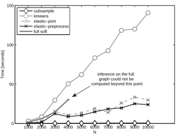
4 Running time for different methods on the SecStr dataset . . . 28
5 Challenges for CAD: 1) fringe and 2) isolated points . . . 37
6 Estimating class-conditional probabilities from two similarity graphs . . . 39
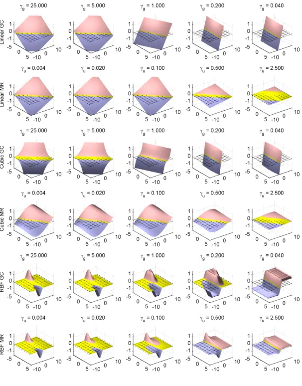
7 Linear, cubic, and RBF decision boundaries for different methods . . . 49
8 The thresholded empirical risk . . . 53
9 Estimating the likelihood ratio from a single graph . . . 63
10 Snapshots from the environment adaptation and office space datasets . . . 67
11 Face-based authentication dataset (left) and examples of labeled faces (right). 68 12 Comparison of SVMs, GC and MR on 3 datasets from the UCI ML repository . 68 13 Coil and Car datasets from UCI ML Repository . . . 72
14 UCI ML: Quality of approximation as a function of time . . . 73
15 UCI ML: Quality of approximation as a function of number of centroids . . . . 74
16 Comparison of 3 face recognizers on 2 face recognition datasets . . . 75
17 Speedups in the total, inference, and similarity computation times . . . 76
18 The three synthetic datasets with known underlying distributions . . . 79
19 Processing of data in the electronic health record . . . 80
20 Examples of temporal features for continuous lab values . . . 82
21 The weight matrix for 100 negative and 100 positive cases of HPF4 order . . . 85
23 Conditional anomaly detection on a synthetic Core dataset . . . 89
24 Histogram of alert examples in the study according to their alert score. . . 91
25 The relationship between the alert score and the true alert rate . . . 93
26 Histogram of anomaly scores for 2 different tasks . . . 94
27 Medical Dataset: Varying graph size . . . 95
LIST OF ALGORITHMS
1 Quantized semi-supervised learning with principal manifolds . . . 27
2 Online quantized harmonic solution . . . 30
LIST OF EQUATIONS
3.1 Closed form solution for a stationary distribution of the random walk.. . . 19
3.5 Soft harmonic solution . . . 21
3.6 Closed form for the soft harmonic solution. . . 21
3.8 Quantized unconstrained regularization . . . 24
3.9 Joint quantization and soft harmonic solution . . . 25
3.10 Quantization step . . . 26
3.11 Approximate quantization step . . . 26
3.12 Solution for the quantization step . . . 26
4.1 Expected value of the n-th order statistic for the standard normal . . . 35
4.2 Posterior probability estimation from a random walk . . . 38
4.3 Regularization of the discriminative approach for CAD . . . 40
4.4 Confidence from the soft label . . . 42
4.5 Anomaly score for soft harmonic anomaly detection . . . 42
4.6 Soft harmonic solution using matrix inversion . . . 43
4.7 Soft harmonic solution using system of linear equations . . . 43
4.8 Compact computation of harmonic solution for the backbone graph . . . 44
5.1 Linear manifold regularization . . . 47
5.3 Linear support vector machine . . . 47
5.4 Risk of our solutions . . . 48
5.5 Empirical risk on graph induced labels . . . 48
5.6 Elastic net . . . 54
5.11 Upper bound on stability of quantized harmonic solution. . . 58
5.12 Upper bound on the quality of quantization . . . 58
5.13 Approximating Laplacian by block-diagonal structure . . . 62
5.14 Approximation bound of block-diagonal structure . . . 62
5.15 Class-conditional probability of a different label . . . 62
5.16 Approximation of the likelihood ratio . . . 63
5.17 Estimation expressed with similarity weights . . . 63
PREFACE
I spent 6 splendid years in Pittsburgh. I want to thank the people who made my journey to PhD possible and enjoyable. First of all, I would like to sincerely thank my advisor Milos Hauskrecht, who made me excited about Machine Learning. With Milos, all my work had a purpose and I was happy to work on important problems that people care about. Therefore, the thought of quitting my PhD (so common among my peers) never crossed my mind. Milos stood by me literally from day one, when he came to pick me up at the airport.
This thesis would not be about graph-based algorithms if not for Brano Kveton, who made me interested in them. He was my mentor during my internships at Intel Research. I am grateful for his friendship and encouragement that made me surpass the expecta-tions I had for myself. Brano is an amazing researcher and he collaborated on many of the semi-supervised learning methods presented here. I would also like to thank my thesis committee, Liz Marai, Diane Litman and in particular John Lafferty, whose research with Jerry Zhu on harmonic functions has laid the foundation for this dissertation.
I was privileged to work with Greg Cooper, who should be a role model for any scientist. He has always impressed me with his professionalism by constantly having a big picture in mind. Greg was a part of a larger interdisciplinary group that I had a great opportunity to work in, ranging from biomedical informaticians to clinicians and pharmacists: Roger Day, who recruited me to the Bayesian club while he played tuba in 7 different bands; Shyam Visweswaran; Amy Seybert; Gilles Clermont; Wendy Chapman; and many others. I would like to thank our post-doc Hamed Valizadegan and Saeed Amizadeh, with whom I worked during my last year, and also other members of Milos’ machine learning lab: Rich Pelikan, Iyad Batal, Shuguang Wang, Quang Nguyen, and Dave Krebs.
taught me a lot about research in the industry. Besides Brano, I would like to thank my research collaborators Ling Huang, Ali Rahimi, Daniel Ting from Berkeley, my colleges Georgios Theocharous, Kent Lyons, Jennifer Healey, John Mark Agosta, Nick Carter, and many other researches and interns.
I also want to thank my teachers from the Machine Learning Department at Carnegie Mellon University, where I learned so much about the field, namely John Lafferty, Larry Wasserman, Carlos Guestrin, Geoff Gordon, Eric Xing, and Gary Miller. I am also grateful to my teachers from Pitt and from Comenius University in Bratislava. But my love for math started with my high school teacher, Martin Macko, who taught me mathematics for 8 years in the best way I can imagine. It is because of him that I decided to do science and research. My mom had a role in that decision, too, and it is probably not a coincidence that she went to grad school for cybernetics.
I am grateful to our administrative staff, who helped to smooth my life at Pitt: Kathy O’Connor, Kathleen Allport, Wendy Bergstein, Loretta Shabatura, Nancy Kreuzer, and Keena Walker. These ladies are running this place and create a feeling like home. Also, I want to thank Phillipa Carter from the Graduate Studies who will remember me as some-body that would stalk her everywhere and would always want to skip the chain of command. Besides my studies, my life in Pittsburgh would not be so great if it was not my friends who made my stay here so enjoyable. I need to mention Tomas Singliar and Zuzana Ju-rigova, Christopher Hughes, Mihai and Diana Rotaru, Roxana and Vlad Gheorgiou for mar-velous times we spent together. I made great friends at Pitt, with whom I would like to keep in touch including Panickos Nephytou, Kiyeon Lee, Ryan Moore, Alexandre Ferreira, Yaw Gyamfi, Samah Mazraani, Weijia Li, Peter Djalaliev, Lory al Moakar, Shenoda Guir-guis, Tatiana Ilina, and also many friends at CMU such as Miro Dudik, Mike Gamalinda, Polo Chau, Kiki Levanti, Michael Papamichael, Jose Gonzales-Brenes, Lucia Castellanos, Mladen Kolar, Stano Funiak, and others.
My time in Pittsburgh was fabulous also due to Pitt Men’s Glee Club, where I sang Tenor 2 at many concerts, including the ones on our tours to Italy, Croatia, and Texas. I need to start with Richard Earl Teaster, the director of the group, who was one of the first people I met upon my arrival to Pittsburgh and over 6 years became one of my best friends.
Besides that he has been my private voice teacher for many of those years and raised me from somebody with almost no experience in singing to a singer in this exquisite ensemble. The glee club became a huge part of me, and my life often consisted of research, friends and glee club. Moreover, within the group I made great friends, such as Mike Pollock, Matt (and Kelly) Keeny, Dexter Gulick, Chad Slyman, Geoff Arnold, Paul Schillenger, Evan Pavloff, Joel Arter, Adam Sloan, Greg Hill, Phil Slane, Tyler Kirland, Ryan McGinnis, Ben Dichter, Josh Niznik, Matt Recker, Matt Cahalan, James Montgomery, Nick Czarnek, Erick Markley, Jared Wilson, Victor Bench, John Moriarty, Mark Ellenberger, Charlie Eichman, Evan McCullough, Evan Williams, and dozens of others with whom I shared the world of music, including my music teachers: Don Fellows, John Goldsmith, Claudia Pinza, Jim Ferla, Sister Maria Ozah, and Ben Harris.
For the most of my time at Pitt, I lived in a big house a few minutes away from my department. Since we often housed visiting students and scholars, during the five years I probably had more than 50 housemates. I will always remember the parental caring of Kevin and Elizabeth Leichbach, dancing robotic toys of David Palmer, delicious food of Az-zurra Missinato and Kikumi Ozaki, Sera Wang, Sonia Wu, Michael Wasilewski, and many others who lived at 307 Halket Street. Through Kevin and Elizabeth to have I met many nice people, such as Kirsten Ream, Kate Shaughnessy, Kelly Reed, George and Becky Maza-gieros, and Bob Fratto. I made many friends at the Pittsburgh branch of Campus Crusade for Christ. The ones that stand out are Matt Budavich, TJ Laird, Zach Fogel, Joe Rathbun, Justin Cooper, and Evelyn Yarzebinski, who made sure that this dissertation is actually written in English.
I would also like to thank my friends in Slovakia, who were often welcoming me at home during my summer and winter breaks and spent time with me on hikes, travels and music festivals. Notably, I would to thank Michal Rjasko for the long years of great friendship. Finally, I am indebted to my family, in particular to my mom Maria, my dad Michal, and my sister Zuzka, who provided me with everything I needed and supported me throughout all my studies. I also thank my extended family, especially my only living grandparent, Anna, who has been praying for me every single day. Her prayers were definitely heard as God gave me the strength and grace I needed.
1.0 INTRODUCTION
1.1 MOTIVATION
If we want people to enjoy the benefits of machine learning, we should provide them with algorithms that do not require much training time before they can be useful. Therefore, we will investigate the algorithms that need only minimal feedback from the users. For example, in semi-supervised learning we assume that only very few examples from the data are labeled and we try to use the unlabeled examples to learn something about the structure of the data. In the area of conditional anomaly detection and in particular in medicine, a traditional approach is to ask experts to create a set of rules that would raise an alert if an adverse event is encountered. Since a manual creation of rules is very time consuming, we would rather like to learn what the adverse event might be from the collection of the past data.
In this dissertation, we will take advantage of using a similarity graph as the data rep-resentation. Similarity graphs help us model the relationship between the examples. How-ever, graph-based algorithms, such as label propagation, do not scale well beyond several thousand examples. We will address this problem by data quantization, where unlike other approaches (k-means, subsampling) we consider the quality of the inference. Moreover, we investigate an online learning formulation of semi-supervised learning, which is suitable for adaptive machine learning systems when the data arrive in a stream.
Furthermore, we extend graph-based learning to conditional anomaly detection prob-lem and apply it to clinical scenarios. Traditionally, anomaly detection techniques identify unusual patterns in data. In clinical settings, these may concern identification of unusual patients, unusual patient–state outcomes, or unusual patient-management decisions.
1 Age Do sa ge of a d rug Conditional Anomaly (Unconditional) Anomaly (Unconditional) Anomaly
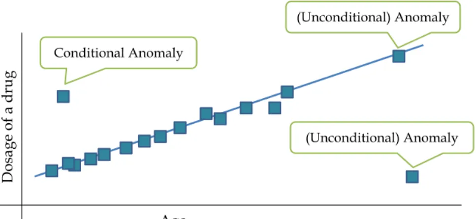
Figure 1: Conditional vs. unconditional anomalies
Our ability to detect unusual events in clinical data may have a tremendous impact on health care and its quality. First, the identification of an action that differs from an expected or usual pattern of care can aid in detection and prevention of the potential medical errors. According to the HealthGrades study (Wall Street Journal on July 27, 2004), medical errors account for 200,000 preventable deaths a year. Second, the identification of anomalous patient responses can help us to identify new promising treatments.
Typical anomaly detection methods used in data analysis are unconditional (with re-spect to the context) and look for outliers with rere-spect to all data attributes. In the medical domain these methods would identify unusual patients, that is, patients suffering from a less frequent disease or patients with unusual collection of symptoms. Unfortunately, this does not fit the nature of the problem we want to solve in error detection: the identification of unusual patient management decisions with respect to past patients who suffer from the same or similar condition. To address this, we are developing a qualitatively new conditional anomaly detection framework where the decision event is judged anomalous with respect to the patient’s symptoms, state, and demographics.
The conditional anomaly detection is the problem of detecting unusual values for a sub-set of variables given the values of the remaining variables. Figure1illustrates the concept of conditional anomaly: Assume that the dosage of a drug is a linear function of the age.
+
+
+
+
+
+
a
b
c
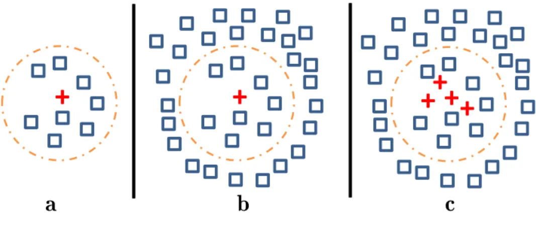
Figure 2: Disadvantages of nearest neighbor approach for conditional anomaly detection
Now imagine that we have a young patient that was given a higher dosage of a drug (Fig-ure1, top left). The amount of dosage is not unusual at all. Indeed, we have other patients with the same or similar dosage. What is unusual is the dosage with respect to his age; the patients that have similar ages were given lower dosages. We can say that this dosage was conditionally anomalous given a patient’s age.
Throughout this dissertation, we build on label propagation on a data similarity graph, which exploits the manifold assumption [Chapelle et al., 2006]. Unlike local neighborhood methods based on the nearest neighbors, it respects the structure of the manifold and lets us account for more complex interactions in the data. In other words, while the metric may provide a reasonable local similarity measure, it is frequently inadequate as a measure of global similarity [Szummer and Jaakkola, 2001]. Figure2 illustrates a potential benefit of label propagation, where the goal is to detect that the positive (+) example has an anomalous label conditioned on its placement. The positive (+) label in2b is more anomalous than the one in2a, but nearest neighbor (NN) would consider them equal, because in only considers the points within the displayed circle. Moreover, the NN approach would find clustered (+) anomalies in2c normal because it ignores the data beyond the nearest neighbors.
1.2 THESIS STATEMENT AND MAIN CONTRIBUTIONS
Although very popular, label propagation on a data similarity graph does not scale well beyond several thousand of examples, due to the following reasons:
1. The computation of the similarity matrix and the label propagation areΩ(n2) where n is the number of examples. Label propagation itself requires the computation of the n × n matrix inverse or the solution of the system of n linear equations.
2. Current methods that reduce the size of the graph to form an approximate back-bone graph do not link the construction of this graph to the final inference task.
3. Despite the usefulness of the online semi-supervised learning paradigm for practical adaptive algorithms, there is not much success in applying this paradigm to realistic problems, especially when data arrive at a high rate.
Next, the problem of conditional anomaly detection could be approached by
1. extending one-class (unconditional) anomaly methods (Section4.4)
2. classification and claiming misclassified examples as conditionally anomalous (Section4.5)
Both of these approaches suffer from the problems of isolated and fringe points described in Section 4. In this dissertation we develop the methodology to address these problems. We take a graph-based approach, because it is non-parametric, incorporates the manifold assumption, and can also easily take advantage of unlabeled data. We present the following main contributions:
• We show how to combine max-margin and semi-supervised learning to max-margin graph cuts semi-supervised learning (Section 3.3).
• We show how to compute label propagation on a graph and the centroids of a backbone graph jointly. (Section3.4)
• We propose the online harmonic function solution and show how to compute its ap-proximation efficiently (Section3.5).
• We prove performance bounds for our online algorithm in a semi-supervised setting on quantized graphs (Section5.4).
• We introduce non-parametric graph-based methods and show how they can handle unconditional outliers (Section4.6).
• We show how a soft harmonic solution on data similarity graphs can be used for conditional anomaly detection (Section4.6.2).
In addition, we test the conditional anomaly detection methods by comparing them to the evaluations conducted with a panel of physicians and show the benefits of our methods (Section6.2.5.1). Based on the aforementioned contributions, we claim the following:
Our graph-based methods can perform online semi-supervised
learning with a constant per-step update and provable performance
guarantees. Moreover, they can detect conditional anomalies and
lter unconditional anomalies.
1.3 ORGANIZATION OF THE DISSERTATION
• In Chapter 2, we outline the related work in anomaly detection (Section 2.3), semi-supervised learning (Section2.2), and graph quantization (Section 2.1).
• Chapter3 presents new approaches for supervised learning and the online semi-supervised learning (Section3.5).
• Chapter4presents novel methods for conditional anomaly detection.
• Chapter5 presents the theoretical analysis of the methods from Chapter 3 and Chap-ter4. In particular, it presents the analysis of max-margin graph cuts (Section5.2) and the analysis of the online semi-supervised learning on quantized graphs (Section5.4). • Chapter6presents the experimental results on various synthetic and real-world datasets,
notably the face recognition video datasets and the medical datasets from University of Pittsburgh Medical Center.
Parts of this dissertation have previously appeared in [Hauskrecht et al., 2007,Hauskrecht et al., 2010,Valko et al., 2008, Valko and Hauskrecht, 2008, Valko and Hauskrecht, 2010,
2.0 RELATED WORK
In this chapter we review the relevant work on graph quantization, semi-supervised learn-ing, and anomaly detection.
2.1 RELATED WORK IN GRAPH QUANTIZATION
Given n data points and a typical graph construction method, the exact computation of the harmonic solution has space and time complexity ofΩ(n2) in general due to the construction of an n×n similarity matrix. Furthermore, exact computation requires an inverse operation on an n × n similarity matrix which takes O(n3) in most practical implementations1. For applications with large data size (e.g., exceeding thousands), the exact computation or even storage of the harmonic solution becomes infeasible, and problems with n in the millions are entirely out of reach.
An influential line of work in the related area of graph partitioning approaches the computation problem by reducing the size of the graph, collapsing vertices and edges, par-titioning the smaller graph, and then uncoarsening to construct a partition for the original graph [Hendrickson and Leland, 1995,Karypis and Kumar, 1999]. Our work is similar in spirit but provides a theoretical analysis for a particular kind of coarsening and uncoarsen-ing methodology.
Our aim is to find an effective data preprocessing technique that reduces the size of the data and coarsens the graph [Madigan et al., 2002,Mitra et al., 2002]. There are two types of approaches widely used in practice for data preprocessing:
1The complexity can be further improved toO(n2.376
1. data quantization based methods, which aim to replace the original data set with a small number of high quality ‘representative’ points that capture relevant structure [Goldberg et al., 2008,Yan et al., 2009];
2. Nyström method based methods, which aim to explore low-rank matrix approximations to speed up the matrix operations [Fowlkes et al., 2004]).
While it is useful to define such preprocessors, it is not satisfactory to simply reduce the size of similarity matrix to speed up the matrix calculations. so that the related matrix operation can be performed in a desired time frame.
What is needed is an explicit connection between the amount of data reduction that is achieved by a preprocessor and the subsequent effect on the classification error. Some widely used data preprocessing approaches are based on data quantization, which replaces the original data set with a small number of high quality centroids that capture relevant structure [Goldberg et al., 2008,Yan et al., 2009].
Such approaches are often heuristic and do not quantify the relationship between the noise induced by the quantization and the final prediction risk. An alternative approach to the computation problem is the Nyström method, a low rank matrix approximation method that allows faster computation of the inverse. This method has been widely adopted, par-ticularly in the context of approximations for SVMs [Drineas and Mahoney, 2005,Williams and Seeger, 2001,Fine and Scheinberg, 2001] and spectral clustering [Fowlkes et al., 2004]. However, since the Nyström method uses interactions between subsampled points and all other data points, storage of all points is required and thus, it becomes unsuitable for infinitely streamed data. To our best knowledge, we are not aware of any online version of Nyström method that could process an unbounded amount of streamed data. Additionally, in an offline setting, the approaches based on the Nyström method have inferior perfor-mance to the quantization-based methods, if both of them are given the same time budget for computation. This was shown in an early work on the spectral clustering [Yan et al., 2009].
Using incremental k-centers [Charikar et al., 1997] which has provable worst case bound on the distortion, we quantify the error introduced by quantization. Moreover, using regu-larization we show that the solution is stable, which gives the desired generalization bounds.
An interesting method is introduced in [Aggarwal et al., 2003], which addresses context drift, or evolution in the data streams. Clusters can emerge and die based on approximated recency. But again this method is a heuristic and comes with no guarantees on the quality of the quantization.
2.2 RELATED WORK IN SEMI-SUPERVISED LEARNING (SSL)
[Zhu et al., 2003] extend their previous work [Zhu et al., 2003] to Gaussian processes by no longer assuming that soft labels are fixed to the observed data. Instead they assume the data generation process x → y → t, where y → t is a noisy label generation with process modeled by a sigmoid. The posterior is not Gaussian and the authors use Laplace approx-imation to compute p(yL, yU|tL). They discuss using different kernels for the learning of
graph weights, such as the tanh-weighted graph, and optimize it either by maximizing the likelihood of labeled data or maximizing the alignment to labeled data.
[Fergus et al., 2009] use the convergence of the eigenvectors of the normalized Laplacian to eigenfunctions of weighted Laplace-Beltrami operators to scale graph-based SSL to mil-lions of examples. Assuming that the underlying distribution has a product form (which is a reasonable assumption after a PCA projection), they estimated the density using histograms for each dimension independently. Therefore, they only needed to solve d generalized eigen-vector problems on the backbone graph, where d is the dimension of the data. Moreover, they only used the k smallest eigenvectors and subsequently needed to solve only one k × k least squares problem.
2.2.1 Semi-Supervised Max-Margin Learning
Most of the existing work on semi-supervised max-margin learning can be viewed as mani-fold regularization of SVMs [Belkin et al., 2006] or semi-supervised SVMs with the hat loss on unlabeled data [Bennett and Demiriz, 1999]. The two approaches are reviewed in the rest of this section. Let l and u be the sets of labeled and unlabeled data respectively.
As-sume that f is a function from some reproducing kernel Hilbert space (RKHS)HK, and k·kK
is the norm that measures the complexity of f .
2.2.1.1 Semi-supervised SVMs Semi-supervised support vector machines with the hat lossV ( f , x) = max{1 − |f (x)|,0} on unlabeled data [b Bennett and Demiriz, 1999]:
min f X i∈l V ( f , xi, yi) + γkf k2K+ γu X i∈u b V ( f , xi) (2.1)
compute max-margin decision boundaries that avoid dense regions of data. The hat loss makes the optimization problem non-convex. As a result, it is hard to solve the problem optimally and most of the work in this field has focused on approximations. A comprehensive review of these methods was done by [Zhu, 2008].
In comparison to semi-supervised SVMs, learning of max-margin graph cuts (3.7) is a convex problem. The convexity is achieved by having a two-stage learning algorithm. First, we infer labels of unlabeled examples using the regularized harmonic function solution, and then we minimize the corresponding convex losses.
2.2.1.2 Manifold regularization of SVMs Manifold regularization of SVMs [Belkin et al., 2006]: min f ∈HK X i∈l V ( f , xi, yi) + γkf k2K+ γufTLf, (2.2)
where f = (f (x1), . . . , f (xn)), computes max-margin decision boundaries that are smooth in
the feature space. The smoothness is achieved by the minimization of the regularization term fTLf. Intuitively, when two examples are close on a manifold, the minimization of fTLf
2.2.2 Online Semi-Supervised Learning
The online learning formulation of SSL is suitable for adaptive machine learning systems. In this setting, a few labeled examples are provided in advance and set the initial bias of the system while unlabeled examples are gathered online and update the bias continuously. In the online setting, learning is viewed as a repeated game against a potentially adversarial nature. At each step t of this game, we observe an example xt, and then predict its label
ˆyt. The challenge of the game is that after it started we do not observe the true label yt.
Thus, if we want to adapt to changes in the environment, we have to rely on indirect forms of feedback, such as the structure of data.
Despite the usefulness of this paradigm for practical adaptive algorithms [Grabner et al., 2008,Goldberg et al., 2008], there is not much success in applying this paradigm to realistic problems, especially when data arrive at a high rate such as in video applications. [Grabner et al., 2008] applies online semi-supervised boosting to object tracking, but uses a heuris-tic method to greedily label the unlabeled examples. This method learns a binary classi-fier, where one of the classes explicitly models outliers. In comparison, our approach is multi-class and allows for implicit modeling of outliers. The two algorithms are compared empirically in Section 6.1.5. [Goldberg et al., 2008] develop an online version of manifold regularization of SVMs. Their method learns max-margin decision boundaries, which are additionally regularized by the manifold. Unfortunately, the approach was never applied to a naturally online learning problem, such as adaptive face recognition. Moreover, while the method is sound in principle, no theoretical guarantees are provided.
[Goldberg et al., 2011] combine semi-supervised learning and active learning in a uni-fied framework. Unlike our work which builds on manifold assumption, they exploit cluster (or gap) assumption, [Chapelle et al., 2006]. The authors present a Bayesian model for this learning setting and use a sequential Monte Carlo approximation for efficient online Bayesian update.
2.3 RELATED WORK IN ANOMALY DETECTION (AD)
2.3.1 Unconditional Anomaly Detection
In this section we review previous approaches for traditional anomaly detection. Traditional anomaly detection looks for examples that deviate from the rest of the data if they are not expected from some underlying model. A comprehensive review of many anomaly detection approaches can be found in [Markou and Singh, 2003a] and [Markou and Singh, 2003b].
[Scholkopf et al., 1999] proposed the one-class SVM, that only needs positive (or non-anomalous) examples to learn the margin. The idea is that the space origin (zero) is treated as the only example of the ‘negative’ class. In that way, the learning essentially estimates the support of the distribution. The data that do not fall into this support have negative projections and can be considered anomalous.
[Eskin, 2000] assumes that the number of anomalies is significantly lower than the number of normal cases. The author defines a distribution for the data as a mixture of major-ity (M) and anomalous distribution(A): D = (1−λ)M +λA. He then iteratively partitions the dataset into the majority set Mtand the anomalous set At. At the beginning A0= ;, M0= D.
At each step t, it is determined whether the case xt is an anomaly. xt is considered
anoma-lous if its displacement to the anomaly set (Mt= Mt−1\ {x} and At = At−1∪ {x}) increases
the log-likelihood LLt−1 of the dataset by a predefined threshold c. If LLt− LLt−1 ≤ c, xt
remains marked as a normal case (Mt= Mt−1 and At= At−1). At the end, we get the final
partition of D into a normal set and an anomalous set.
The curse of high dimensionality is of concern in [Aggarwal and Yu, 2001]. The authors search for the abnormal lower dimensional projections by dividing each attribute into the equi-depth (the same range of f cases) ranges. Assuming statistical independence, each k-dimensional sub–cube in this grid should contain the fraction of fk of total cases. The au-thors then search for k-dimensional sub-cubes, where the presence of points is significantly lower than expected. As the brute force search for projections is computationally infeasible, the authors use genetic algorithms to perform the search.
neighbor) to get the so–called reachability distance for the object O with respect to p as reach_dist(O, p) = max(k_distance(p),dist(O, p)). Using this smoothed distance, they define the local outlier factor (LOF), which expresses the degree of the considered object being an outlier with respect to its neighborhood. LOF depends on M inP ts, the number of nearest points to define a local neighborhood. Although this is data-dependent, the authors propose to calculate the maximum LOF for M inP ts within a reasonable range (which was 30–50 in their experiments) and threshold. The bigger the LOF the more anomalous the object is. The authors give bounds for LOF and prove they are tight for important cases. For example, LOF is close to one for objects within the clusters. A useful property of LOFs is that it works well with cluster of different densities.
[Lazarevic and Kumar, 2005] applies a bagging approach to improve the performance of local (nearest neighbor) anomaly detectors. In every round of the algorithm a subset of features is selected and a local anomaly detector (such as LOF [Breunig et al., 2000]) is applied. Every round produces a scoring of all data, which is at the end merged to get a final score using either breadth-first or cumulative-sum approach.
[Syed and Rubinfeld, 2010] use a minimum enclosing ball approach to detect anomalies in clinical data similar to the data that we use in this work. The authors learn a minimum volume hypersphere that encloses the data for all patients. The anomaly score is defined as the distance from the center. They showed that this unsupervised approach performed similarly to the supervised approaches with prelabeled examples (Section2.3.1.1).
[Akoglu et al., 2010] performs anomaly detection on weighted graphs when nodes do not follow discovered power laws between the number of neighbors and the properties of the local neighborhood subgraph (total number of edges, total weight, and the principal eigenvalue of the weighted adjacency graph). The outlier score is defined as a distance to the fitting line. To account for the points that fit the line but are far away from all other examples, the authors combine their methods with a density based method, such as LOF [Breunig et al., 2000].
[He et al., 2007] is a semi-supervised method that propagates the labels until a heuristic stopping criterion is reached. Moreover, it uses unlabeled data to better estimate the prior in the case that the empirical distribution is skewed from the true distribution.
[Moonesignhe and Tan, 2006] use random walks to detect outliers. They build their sim-ilarity matrix either by cosine simsim-ilarity or by a number of shared neighbors after thresh-olded cosine similarity. Anomalous nodes are identified as those with low connectivity. Con-nectivity is calculated using the Markov chain with the similarity as a transition matrix. Starting from the uniform connectivity assigned at step 0, connectivity is spread according to the similarity matrix until convergence.
2.3.1.1 Approaches with prelabeled anomalies [Chawla et al., 2003] combine a boost-ing scheme with SMOTE (Synthetic Minority Over-samplboost-ing TEchnique). They do that in every iteration of smoothing. For continuous data, SMOTE generates a new sample by sam-pling a data point and one of its k nearest neighbors and taking a random point on segment between them in the space. For discrete data, a new point is created as a majority vote of the k nearest neighbors for each feature. The authors show improvement with this method over just smoothing, just SMOTE and applying SMOTE once before the boosting for a minority class. The SMOTEboost approach generally improves recall but does not cause significant degradation in precision, thus improving the F-measure.
[Ma and Perkins, 2003] use support vector regression to learn the underlying temporal model (time event is modeled as a linear regression function of the previous events). A surprise is defined as the value outside the tolerance range. Given the fixed length of the event, a probability of number of surprises actually happing is calculated. When that is too small, an anomaly is declared.
2.3.1.2 Rare category detection [Pelleg and Moore, 2005] aim to detect rare category which presumably correspond to the interesting anomalies in a pool-based active learning framework. After a human expert labels some examples, the Gaussian mixture is fit to the data. Different hinting heuristics are then used to propose the new examples to be labeled by the expert. The authors propose interleave heuristics which takes one example per mixture a time with low fit probability, not taking to account any mixture weight. This heuristic appears to be superior to the low-likelihood one (suggesting examples with the overall low fit probability) and ambiguous one (suggesting examples with uncertain class membership).
[He and Carbonell, 2008] attempt to detect rare categories in the data, assuming that examples from the rare category are self-similar, tightly grouped, and we have some knowl-edge about the class priors. The nearest neighbor based statistic is used to actively sample points corresponding to points with the maximum change in the local density.
2.3.2 Conditional Anomaly Detection (CAD)
We start with a short summary of our work. In [Hauskrecht et al., 2007], we introduce the concept of the conditional anomaly detection (CAD) and show its potential for the medical records. For each case, we take its nearest neighbors and learn a Bayesian belief network (BBN) or a naïve Bayes model (NB) from them. The cases with low class-conditional prob-abilities were deemed anomalous. We discovered that while for BBN it was better to use all the cases for learning, for a more restricted NB a small neighborhood was beneficial. The main problem with learning the structure of BBN is that it does not scale beyond a couple dozen features. In [Valko and Hauskrecht, 2008], we show the benefit of distance metric learning for the selection of closest cases. We also use the softmax model [Mccullagh and Nelder, 1989] to calculate the class-conditional probability of a probabilistic one near-est neighbor (similar to [Goldberger et al., 2004]) for this purpose. In [Valko et al., 2008], we introduce a new anomaly measure based on the distance from the hyperplane learned by SVM [Vapnik, 1995] and perform the initial experiments on the PCP (Section 6.2.2) dataset. We later conduct an extensive human evaluation study with a panel of 15 physi-cians in [Hauskrecht et al., 2010]. Aside from our work which will be reviewed in more detail in later chapters, we also describe other early work along these lines.
[Valizadegan and Tan, 2007] use the kernel based weighted nearest neighbor approach to jointly estimate the probabilities of the examples being mislabeled. The joint estimation is posed as an optimization problem and solved with Newton methods. A regularization is needed to avoid one of the classes deemed to be completely mislabeled.
In [Song et al., 2007], a user defines a partitioning of the features into two groups: the indicator features — those that can be directly indicative of an anomaly and the environ-mental features, which cannot, but can influence the indicator features. The indicator ( y)
and the environmental (x) variables are modeled separately both as the mixtures of multi-variate Gaussians ( y ∼ U and x ∼ V ). A mapping function is defined between those mixtures as the probability of choosing a Gaussian for an indicator variable given an environmental one p(Vj|Ui). The authors assume the following generative process for a datapoint 〈x, y〉: If
x is a sample from Ui then a die is tossed, according to p(Vj|Ui), to determine which
Gaus-sian from V will produce y and subsequently y is produced. Since it is not known, which Ui
the x was sampled from, the likelihood of fC AD( y|Θ, x) is computed as a weighted sum over
Gaussians Ui. The model is learned via EM, either directly — optimizing all parameters at
once (named as DIRECT), optimizing first parameters for Gaussians and then for the map-ping function (FULL), or optimizing the indicator Gaussians, the environmental Gaussians and the mapping function separately (SPLIT).
The work on cross-outlier detection [Papadimitriou and Faloutsos, 2003] is also related to CAD. Papadimitriou and Faloutsos [Papadimitriou and Faloutsos, 2003] defined the no-tion of the cross-outliers as examples that seem normal when considering the distribuno-tion of examples from the assigned class, but are abnormal when considering the samples from the other class. For each sample (x, y), they compute two statistics based on the similarity of x to its neighborhood from the samples belonging to class y and samples not belonging to class y. An example is considered anomalous if the first statistic is significantly smaller than the second statistic. Unfortunately, the method is not very robust to fringe points (Figure5) [Papadimitriou and Faloutsos, 2003].
In his dissertation, [Das, 2009] aims to detect several kinds of individual and group anomalies. The approaches relevant to this work are conditional and marginal methods for individual record anomalies, ignoring rare values. For the data t and the subsets of attributes (A, B, C) he computes the ratios of the form P(A)P(B)P(A,B) for the marginal method and P(A|C)P(B|C)P(A,B|C) for the conditional method. The goal is to find unusual occurrences of the attribute values. The records that have low ratios are considered anomalous. The normal-ization of the joint probabilities by the marginal provabilities takes care of rare records, because those also have small marginals. The dissertation describes several speedups to compute the ratios for exponentially many subgroups to allow the methods to scale up.
3.0 SEMI-SUPERVISED LEARNING
Semi-supervised learning (SSL) is a field of machine learning that studies learning from both labeled and unlabeled examples. This learning paradigm is suitable for real-world problems, where data is often abundant but the resources to label them are limited. As a result, many semi-supervised learning algorithms have been proposed in the past few years [Zhu, 2008]. The closest to this work are semi-supervised support vector machines (S3VMs) [Bennett and Demiriz, 1999], manifold regularization of support vector machines (SVMs) [Belkin et al., 2006], and harmonic function solutions on data adjacency graphs [Zhu et al., 2003].
SSL is very closely related to transductive inference (Chapters 24 and 25 in [Chapelle et al., 2006]). In both approaches we have access to the unlabeled examples that we can take advantage of. Traditionally in SSL, we want to use the unlabeled data to learn a function f that can be later used to classify previously unseen examples. We present one such approach where we combine the harmonic solution on a data similarity graph with a max-margin inference in Section 3.3. In other scenarios, we may not need to learn such a function. In this case, we can focus just on classifying the unlabeled examples at hand. Even then, the prediction on unseen examples is still possible using out of sample extension methods [Bengio et al., 2004].
In this dissertation we study graph-based methods for SSL, because they can model complex interactions between the examples. However, graph-based methods (such as label propagation) do not scale beyond several thousand examples unless we use parallel archi-tectures. One of the solutions is to reduce the number of nodes and create a representa-tive back-bone graph. Typically, one can downsample the data or use some quantization technique (such as k-means) to come up with a smaller graph. Yet these approaches do
not consider the quality of semi-supervised learning inference for this backbone graph. In Section 3.4 we introduce a new objective function that lets us incorporate the quality of inferences into the construction of the backbone graph.
Furthermore, in Section3.5we investigate an online learning formulation of SSL, which is suitable for adaptive machine learning systems. In this setting, a few labeled examples are provided in advance and set the initial bias of the system, while unlabeled examples are gathered online and update the bias continuously. In the online setting, learning is viewed as a repeated game against a potentially adversarial nature. At each step t of this game, we observe an example xt and then predict its label ˆyt. The challenge of the game is that after
it started we do not observe the true label yt. Thus, if we want to adapt to changes in the
environment, we have to rely on indirect forms of feedback, such as the structure of data. When data arrive in a stream, the dual problems of computation and data storage arise for any SSL method. We therefore propose a fast approximate online SSL algorithm that solves for the harmonic solution on an approximate graph.
For all our methods, we introduce the regularized harmonic solution (Section 3.2) to achieve better stability properties. With such regularization, we can control the confidence of labeling unlabeled examples and discount the outliers in the data. In the following, we start with some needed background in graph theory and then continue with the just men-tioned approaches for SSL.
3.1 GRAPHS AS DATA MODELS
Many of the methods presented here are based on a graph representation of the data. Hav-ing some data, we create a undirected weighted graph G = (V , E) with set of vertices V and set of edges E, associating every data point with a graph vertex. Next, we define a non-negative weight function V ×V → R such that wi j= wji. In the case that {i, j} ∉ E(G), wi j= 0.
Let the similarity matrix W = {wi j} denote a matrix of all edge weights which encode how
similar the vertices are to each other. We define degree di of the vertex i as the sum of all
di=X
j
wi j
and the diagonal matrix D with Dii= di. Let volume vol(G) of graph G be the sum of all its
weights: vol(G) = vol(W) =X i di= X i, j wi j
Now, let us define an unnormalized graph Laplacian L as
L(G) = L(W) = D − W
and the symmetric normalized graph Laplacian as
Lsym(G) = Lsym(W) = D− 1 2LD− 1 2 = I − D− 1 2W D− 1 2.
It can be easily shown that for any h ∈ Rn:
hTLh =1 2
X
i j
wi j(hi− hj)2.
3.1.1 Stationary Distribution of a Random Walk
Here we describe a way to compute a stationary distribution of a (non-absorbing) random walk on the data similarity graph in a closed form. Let us define the random walk as follows: In every step of a random walk, we jump from a node to its neighbors, proportionally to their mutual weight:
P(xi→ xj) =
Wi j
P
j0Wi j0
Let D be the diagonal matrix with the sum of weights W on the diagonal: Dii=Pj0Wi j0 for
all i. The transition matrix of this random walk is P = D−1W. The approximation we use here is that we estimate the class conditional probability with the proportion of the time that the random walk spends in the evaluated example [Lee and Wasserman, 2010]. We can calculate this proportion from the stationary distribution of this random walk [Chung,
1997]. Let s be a row vector of the stationary distribution of a random walk with the transi-tion matrix P. For a statransi-tionary distributransi-tion s, it has to hold that sP = s. Note that 1D = 1W, where 1 is all one row vector. It is easy to verify that
s = 1W
vol(W) (3.1)
satisfies the definition:
sP = 1W P vol(W)= 1DP vol(W)= 1DD−1W vol(W) = 1W vol(W)= s
The equation (3.1) enables us to compute the stationary distribution in a closed form.
3.2 REGULARIZED HARMONIC FUNCTION
In this section, we build on the harmonic solution [Zhu et al., 2003]. Moreover, we show how to regularize it such that it can interpolate between semi-supervised learning (SSL) on labeled examples and SSL on all data. A standard approach to SSL on graphs is to minimize the quadratic objective function
min
`∈Rn `
TL`
(3.2)
s.t. `i= yi for all i ∈ l;
where` denotes the vector of predictions. Using the notation from Section3.1, this problem has a closed-form solution:
`u= (Duu− Wuu)−1Wul`l,
which satisfies the harmonic property`i=d1iPj∼iwi j`j(i ∼ j denotes that i neigbors j), and
therefore is commonly known as the harmonic solution. Since the solution can be also computed as:
it can be viewed as a product of a random walk on the graph W with the transition matrix P = D−1W. The probability of moving between two arbitrary vertices i and j is wi j/di, and
the walk terminates when the reached vertex is labeled. Therefore, the harmonic solution is a form of label propagation on the data similarity graph. Each element of the solution is given by: `i = (I − Puu)−1iuPul`l = X j: yj=1 (I − Puu)−1iuPu j | {z } p(+1)i − X j: yj=−1 (I − Puu)−1iuPu j | {z } p(−1)i = p(+1)i − p(−1)i ,
where p+1i and p−1i are probabilities by which the walk starting from the vertex i ends at vertices with labels +1 and −1, respectively. Therefore, when `i is rewritten as |`i| sgn(`i),
|`i| can be interpreted as a confidence in assigning the label sgn(`i) to the vertex i. The
maximum value of |`i| is 1, and it is achieved when either p+1i = 1 or p−1i = 1. The closer
the confidence |`i| is to 0, the closer the probabilities p+1i and p−1i are to 0.5, and the more
uncertain the label sgn(`i) is.
We propose to control the confidence of labeling by regularizing the Laplacian L as L +
γgI, whereγg is a scalar and I is the identity matrix. Similarly to (3.2), the corresponding
problem min `∈Rn ` T (L + γgI)` (3.3) s.t. `i= yi for all i ∈ l;
can be computed in a closed form
`u= (Luu+ γgI)−1Wul`l. (3.4)
and we will refer to it as regularized HS. It can be also interpreted as a random walk on the graph W with an extra sink. At every step, a walk at node xi may terminate at the sink
with probabilityγg/(di+ γg) where di is the degree of the current node in the walk .
decreases with the number of hops from labeled vertices. The proposed regularization will essentially drive the confidence of distant vertices to zero.
3.2.1 Soft Harmonic Solution
A related problem to (3.2) is when the constraints representing the fit to the data are en-forced in a soft manner [Cortes et al., 2008]. In such a case, we are able to bound the generalization error of the solution (Section5.1). Moreover, the soft harmonic solution can be used for label propagation in case of noise labels (Section4.6.2). One way of enforcing the fit constraints in a soft manner is by solving a following problem:
`?= min
`∈Rn(` − y)
T
C(` − y) + `TK`, (3.5)
where K = L + γgI is the regularized Laplacian of the similarity graph, C is a diagonal
matrix such that Cii= cl for all labeled examples, and Cii= cuotherwise, and y is a vector
of pseudo-targets such that yi is the label of the i-th example when the example is labeled,
and yi= 0 otherwise. The appealing property of (3.5) is that its solution can be computed in
closed form as follows [Cortes et al., 2008]:
`?= (C−1K + I)−1y (3.6)
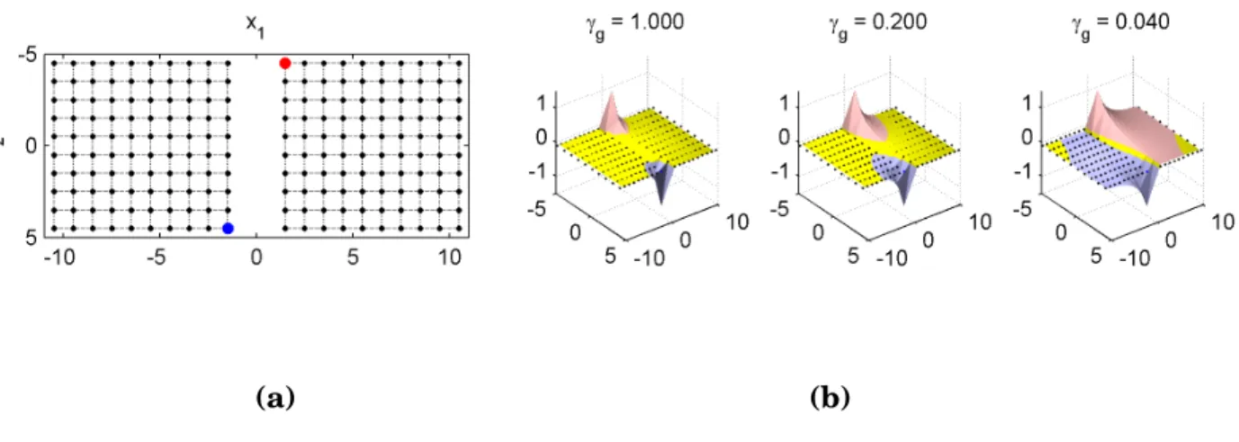
We will use soft harmonic solution (3.5) particularly in the theoretical analysis in Chapter5. Several examples of howγg affects the regularized solution are shown in Figure3.
Fig-ure 3a shows an example of a simple data adjacency graph. The vertices of the graph are depicted as dots. The bigger dots in the middle are labeled vertices. The edges of the graph are shown as dotted lines and weighted as wi j= exp[−
° °xi− xj
° °
2
2/2]. Figure3b. shows three
regularized harmonic function solutions on the data adjacency graph from Figure3a. The plots are cubic interpolations of the solutions. The dark (or pink and blue) colors denote parts of the feature space x where `i > 0 and `i < 0, respectively. The light (or yellow)
color marks regions where the confidence |`i| is less than 0.05. Whenγg= 0, the solution
turns into the ordinary harmonic function solution. Whenγg=∞, the confidence of labeling
in-(a) (b)
Figure 3: a. Similarity graph b. Three regularized harmonic solutions
creasing all eigenvalues of the Laplacian L byγg [Smola and Kondor, 2003]. In Section5.2
we use this property to bound the generalization error of our solutions.
3.3 MAX-MARGIN GRAPH CUTS
In this part we present our algorithm that combines the harmonic solution with max-margin learning to learn a classifier f from some reproducing kernel Hilbert space (RKHS). In the scenarios, where we do not want to store all the examples in the dataset and perform the inference transductively when the new data arrive, we may prefer to learn such f instead. Our semi-supervised learning algorithm involves two steps. First, we obtain the regular-ized harmonic function solution`∗(3.4). The solution is computed from the system of linear equations (Luu+ γgI)`u= Wul`l. This system of linear equations is sparse when the data
adjacency graph W is sparse. Second, we learn a max-margin discriminator, which is con-ditioned on the labels induced by the harmonic solution. The optimization problem is given
by: min f ∈HK X i:¯ ¯`∗ i ¯ ¯≥ε V ( f , xi, sgn(`∗i)) + γkf k2K (3.7) s.t. `∗= arg min `∈Rn` T (L + γgI)` s.t.`i= yi for all i ∈ l;
where V ( f, x, y) = max{1 − yf (x),0} denotes the hinge loss, HK, and k·kK is the norm that
measures the complexity of f .
The training examples {xi}in our problem are selected based on our confidence into their
labels. When the labels are highly uncertain, which means that¯¯`∗
i
¯
¯< ε for some small ε ≥ 0, the examples are excluded from learning. Note that as the regularizer γg increases, the
values¯¯`∗
i
¯
¯decrease towards 0 (Figure3), and theε thresholding allows for smooth interpo-lations between supervised learning on labeled examples and semi-supervised learning on all data. The trade-off between the regularization of f and the minimization of hinge losses V ( f , xi, sgn(`∗i)) is controlled by the parameterγ.
Due to the representer theorem [Wahba, 1999], the optimal solution f∗ to our problem has a special form:
f∗(x) = X i:¯ ¯`∗ i ¯ ¯≥ε α∗ ik(xi, x),
where k(·,·) is a Mercer kernel associated with the RKHS HK. Therefore, we can apply
the kernel trick and optimize rich classes of discriminators in a finite-dimensional space of
α = (α1, . . . ,αn). Finally, note that when γg= ∞, our solution f∗ corresponds to supervised
learning with SVMs.
In some aspects, manifold regularization (Section2.2.1.2) is similar to max-margin graph cuts. In particular, note that its objective (2.2) is similar to the regularized harmonic func-tion solufunc-tion (3.3). Both objectives involve regularization by a manifold, fT
Lf and `TL`,
regularization in the space of learned parameters, kf k2K and `TI`, and some labeling
con-straints V ( f, xi, yi) and `i = yi. Since max-margin graph cuts are learned conditionally
on the harmonic function solution, the problems (3.7) and (2.2) may sometimes have simi-lar solutions. A necessary condition is that the regusimi-larization terms in both objectives are
weighted in the same proportions, for instance, by setting γg= γ/γu. We adopt this setting
when manifold regularization of SVMs is compared to max-margin graph cuts in Section
6.1.3.
3.4 JOINT QUANTIZATION AND LABEL PROPAGATION
Graph-based semi-supervised learning methods do not scale well to large data sets, mainly because their inference procedures require the computation of the inverse of an n×n matrix, where n is the size of the underlying graph that is equal to the size of the dataset. A typical solution to address this problem is to downsize the graph to a smaller backbone graph and perform the inference on this reduced representation. The key challenge is to decide on what elements should be included in the backbone graph. Typical solutions include sub-sampling, clustering, or a Nyström approximation. However, these techniques do not consider the quality of semi-supervised learning inferences for this backbone graph. We introduce a new objective function that lets us incorporate the quality of inferences into the construction of the backbone graph.
To reduce the computational complexity of (3.5), we replace all n nodes of the similarity graph G with a set C = [c1, ...cm, ..., cm+k]T of (m + k) ¿ n representative nodes to create a
backbone graph ˜G. Notice that ci= xi for i = 1,..., m. We want to find ˜G such that it is a
good representation of G in constructing the manifold. Let us assume for a moment that we do know the best set of examples ˜G. Then, Equation (3.5) becomes:
`?= argmin`∈Rn (` − y)TFC(` − y) + `TLC`. (3.8)
In general, C ∈ R(m+k)×d can be obtained by fixing the first m labeled examples and choosing k unlabeled points by subsampling the dataset, clustering or other means of quantization. As mentioned earlier, the common approach is to select the set C first and only then perform the inference (3.8). In this work, we will perform both the quantization and the inference jointly by adding the quantization penalty of the elastic nets to the objective function in (3.8). As we will see in Section5.3, this simple joint approach will produce interesting properties.
The new objective function is: [`?, {cj}m+kj=m+1] = argmin`∈Rn,{c j}m+kj=m+1 (` − y) T FC(` − y) + `TLC` γq à (m + k)2 n X xi∈Kj ||cj− xi||2 ! (3.9) where Kj is the set of examples for which cj is the nearest centroid andγq is a cost
param-eter for the quantization penalty. We emphasize that we automatically consider all labeled examples as a fixed part of C and the optimization to learn the representing centroids are affected by the position of labeled examples. As we will see in Section 5.3, the above objec-tive function has an interesting property: when optimized to find the centroids, it learns the principle manifold.
Adding the quantization penalty makes the objective function non-convex and hence difficult to optimize. To minimize (3.9), we propose to use an alternating optimization ap-proach [Bezdek and Hathaway, 2002], where we alternate between 1) label propagation — inferring labels l on ˜G, and 2) quantization — selecting the set C for ˜G. Starting with random seeds of unlabeled examples (or the output of k-means algorithm) as the initial centroids, we iterate the following steps.
3.4.1 Label Propagation
Once C is fixed, the labels can be computed by solving the following convex optimization problem:
`?= argmin`∈Rn (` − y)TFC(` − y) + `TLC`
This problem has a closed form solution:`?= ((FC)−1LC+ I)−1y (Section3.2).
3.4.2 Quantization
To learn the centroids C when` is fixed, first notice that:
`TLC` =X i, j µl i ni− lj nj ¶2 Wi jC
where (ni = 1)m+ki=1 for unnormalized graph Laplacian L = DC− WC [Luxburg, 2007] and
(ni=pdi)m+ki=1 for normalized graph Laplacian L = I −D−1/2W D−1/2[Zhou et al., 2004].
Con-sidering that (` − y)TFC(` − y) in (3.9) is not dependent on C, we have the following
opti-mization problem to learn C if we use the widely used Gaussian kernel1 as the similarity function W: {cj}m+kj=m+1= argmin{cj}m+k j=m+1 X i, j µl i ni − lj nj ¶2 exp à −||cj− ci||2 2σ2 ! + γq à (m + k)2 n X i∈Kj ||cj− xi||2 ! (3.10) To learn the centers by optimizing (3.10), we first approximate the exponential function using Taylor expansion2:
exp à −||cj− ci||2 2σ2 ! ≈ 1 −||cj− ci|| 2 2σ2 ,
This results in the following optimization problem:
{cj}m+k j=m+1= argmin{cj}m+kj=m+1 −1 (m + k)2 X i, j à (li− lj)2 2σ2 ! ||cj− ci||2+ γq n X i∈Kj ||cj− xi||2 (3.11)
Taking derivatives of (3.11) with respect to (cj)m+kj=m+1and setting them to zero, we obtain the
following system of k linear equations for j = m + 1,..., m + k :
X i ci (li− lj) 2 (m + k)2σ2+ cj à 2γq |Kj| n − X i (li− lj)2 (m + k)2σ2 ! =2γq n X i∈Kj xi, (3.12)
where |Kj| is the number of examples assigned to the center cj. In order to optimize the
system of linear equations in (3.12), we iterate between optimizing the centroids and the assignment of the examples to the centroids, a strategy similar to k-means.
Notice that the labeled examples c1, .., cm affect learning the centroids by
1It is straightforward to apply similar derivation for other similarity functions.
2Notice we could also use the convexity of the exponential function to obtain an upper bound and have
a more rigorous derivation. However, the results are very similar and we omit the details to simplify the description.