HAL Id: tel-01671507
https://hal.inria.fr/tel-01671507
Submitted on 5 Jan 2018HAL is a multi-disciplinary open access archive for the deposit and dissemination of sci-entific research documents, whether they are pub-lished or not. The documents may come from teaching and research institutions in France or abroad, or from public or private research centers.
L’archive ouverte pluridisciplinaire HAL, est destinée au dépôt et à la diffusion de documents scientifiques de niveau recherche, publiés ou non, émanant des établissements d’enseignement et de recherche français ou étrangers, des laboratoires publics ou privés.
polynomial system solving
Anna Karasoulou
To cite this version:
Anna Karasoulou. Algebraic combinatorics and resultant methods for polynomial system solving. Computer Science [cs]. National and Kapodistrian University of Athens, Greece, 2017. English. �tel-01671507�
ΤΜΗΜΑ ΠΛΗΡΟΦΟΡΙΚΗΣ ΚΑΙ ΤΗΛΕΠΙΚΟΙΝΩΝΙΩΝ ΠΡΟΓΡΑΜΜΑ ΜΕΤΑΠΤΥΧΙΑΚΩΝ ΣΠΟΥΔΩΝ ΔΙΔΑΚΤΟΡΙΚΗ ΔΙΑΤΡΙΒΗ
Μελέτη και επίλυση πολυωνυμικών συστημάτων με
χρήση αλγεβρικών και συνδυαστικών μεθόδων
Άννα Ν. Καρασούλου ΑΘΗΝΑ Μάιος 2017DEPARTMENT OF INFORMATICS AND TELECOMMUNICATIONS PROGRAM OF POSTGRADUATE STUDIES
PhD THESIS
Algebraic combinatorics and resultant methods for
polynomial system solving
Anna N. Karasoulou
ATHENS May 2017
συνδυαστικών μεθόδων Άννα Ν. Καρασούλου ΕΠΙΒΛΕΠΩΝ ΚΑΘΗΓΗΤΗΣ: Ιωάννης Ζ. Εμίρης, Καθηγητής ΕΚΠΑ ΤΡΙΜΕΛΗΣ ΕΠΙΤΡΟΠΗ ΠΑΡΑΚΟΛΟΥΘΗΣΗΣ: Ιωάννης Ζ. Εμίρης, Καθηγητής ΕΚΠΑ Ευάγγελος Ράπτης, Καθηγητής ΕΚΠΑ
Bernard Mourrain, Διευθυντή ερευνών Ινστιτούτο INRIA Sophia Antipolis
-Méditerranée ΕΠΤΑΜΕΛΗΣ ΕΞΕΤΑΣΤΙΚΗ ΕΠΙΤΡΟΠΗ Ιωάννης Ζ. Εμίρης, Ευάγγελος Ράπτης, Καθηγητής ΕΚΠΑ Καθηγητής ΕΚΠΑ Bernard Mourrain, Βασίλειος Ζησιμόπουλος, Διευθυντή ερευνών Ινστιτούτο INRIA
Sophia Antipolis - Méditerranée
Καθηγητής ΕΚΠΑ Νικόλαος Μισυρλής, Μιχαήλ Ν. Βραχάτης, Καθηγητής ΕΚΠΑ Καθηγητής Πανεπιστήμιο Πατρών Ilias S. Kotsireas, Καθηγητής Πανεπιστημίο Wilfrid Laurier
Algebraic combinatorics and resultant methods for polynomial system solving
Anna N. Karasoulou
SUPERVISOR: Ioannis Z. Emiris, Professor NKUA THREE-MEMBER ADVISORY COMMITTEE:
Ioannis Z. Emiris, Professor NKUA Evangelos Raptis, Professor NKUA
Bernard Mourrain, Director of Research INRIA Sophia Antipolis -
Méditer-ranée
SEVEN-MEMBER EXAMINATION COMMITTEE
Ioannis Z. Emiris, Evangelos Raptis,
Professor NKUA Professor NKUA
Bernard Mourrain, Vassilis Zissimopoulos,
Director of Research INRIA Sophia An-tipolis - Méditerranée
Professor NKUA
Nikolaos Missirlis, Michael N. Vrahatis,
Professor NKUA Professor University of
Pa-tras
Ilias S. Kotsireas,
Η διδακτορική διατριβή της Άννας Καρασούλου επικεντρώνεται στην επίλυση πολυωνυμι-κών συστημάτων χρησιμοποιώντας εργαλεία από την αλγεβρική και την συνδυαστική γεω-μετρία. Η χρήση συνδυαστικών μεθόδων κατέστη απαραίτητη για την εκμετάλλευση της δομής και της αραιότητας των πολυωνυμικών εξισώσεων. Περιγράφονται επίσης γεωμετρι-κοί αλγορίθμοι για την διάσπαση πολυτόπων κατά Minkowski, με απώτερη εφαρμογή την παραγοντοποίηση των αντίστοιχων πολυωνύμων στο πλαίσιο της εκμετάλλευσης της αραιότητάς τους. Η κ. Άννα Καρασούλου αντιμετώπισε με επιτυχία ορισμένα μη τετριμμέ-να προβλήματα, τα οποία επιγραμματικά ατετριμμέ-ναφέρουμε εδώ και τα ατετριμμέ-ναλύουμε στην συνέχεια. Το πρώτο πρόβλημα είναι ο υπολογισμός τύπου της αραιής απαλοίφουσας (sparse re-sultant) και της αραιής διακρίνουσας (sparse discriminant) [14], [29], [39], με χρήση της δομής των εξισώσεων. Επιπλέον μελετήθηκε και βρέθηκε κλειστός τύπος για τον βαθμό της διακρίνουσας και της απαλοίφουσας πολυωνυμικών εξισώσεων καθώς και η μεταξύ τους σχέση. Ειδικότερα, διενεργήθηκε μελέτη τύπων για τον βαθμό της αραιής (μεικτής) διακρίνουσας και της αραιής απαλοίφουσας πολυωνυμικών εξισώσεων. Ο σκοπός της μελέτης αυτής είναι να διερευνηθεί ο τρόπος υπολογισμού της αραιής διακρίνουσας ενός καλώς ορισμένου συστήματος μέσω ενός τύπου που την συνδέει με την αραιή απαλοίφουσα ενός υπερπροσ-διορισμένου πολυωνυμικού συστήματος, εξετάζοντας τα αραιά πολυώνυμα μέσω της θεω-ρίας των πολυτόπων του Νεύτωνα. Στα πλαίσια της μελέτης αυτής προέκυψαν δύο ερευνη-τικές εργασίες [39], [29], οι οποίες περιγράφονται αναλυτικά στα κεφάλαια 4 και 6. Στο κεφάλαιο 4 μελετάται η σχέση της αραιής διακρίνουσας και της απαλοίφουσας με έμφαση στις εφαρμογές της διακρίνουσας. Μελετάται η σχέση της αραιής διακρίνουσας με την αραιή απαλοίφουσα του συστήματος των πολυωνύμων επαυξημένου με τον Τορικό Ιακωβι-ανό πίνακα του συστήματος. Η σχέση αυτή οδηγεί σε έναν τύπο για την αραιή διακρίνουσα, ο οποίος επιτρέπει τον υπολογισμό της αποτελεσματικά, χωρίς την εισαγωγή νέων μεταβλη-τών, όπως γίνεται με τη μέθοδο του Cayley. Δίνεται επίσης μία απόδειξη για τον συνολικό βαθμό της αραιής διακρίνουσας 2 πολυωνύμων, καθώς και ένας τύπος για την αραιή διακρίνουσα όταν ένα εκ των πολυωνύμων παραγοντοποιείται, χρησιμοποιώντας τα πολύ-τοπα του Νεύτωνα. Στο κεφάλαιο 5 περιγράφεται η μελέτη που διενεργήθηκε , πάνω στην διακρίνουσα των ομογενών συμμετρικών πολυωνύμων, δηλαδή των αναλλοίωτων συστημάτων κάτω από την δράση της συμμετρικής ομάδας. Αναζητήθηκε και βρέθηκε κλειστός τύπος για τον υπολογισμό της απαλοίφουσας και της διακρίνουσας τέτοιου συστήματος. Το δεύτερο πρόβλημα το οποίο αντιμετώπισε είναι το NP-δύσκολο πρόβλημα του υπολογι-σμού της διάσπασης πολυτόπων κατά Minkowski με χρήση προσεγγιστικών [41] και αλγο-ρίθμων ακριβείας [36], καθώς και η μελέτη του προβλήματος του αθροίσματος υποσυνόλων (subset sum) σε αυθαίρετη διάσταση [41].
που διάστασης d, το οποίο έχει κορυφές με ακέραιες συντεταγμένες. Για τον υπολογισμό αυτό μελετήθηκε ο κώνος όλων των συνδυαστικά ισοδύναμων πολυτόπων. Η υλοποίηση δίνεται σε Sage. Στο κεφάλαιο 8 μελετώνται δύο NP-δύσκολα προβλήματα: το πρόβλημα της διάσπασης κατά Minkowski των ακέραιων πολυτόπων στο επίπεδο και το πρόβλημα του αθροίσματος υποσυνόλων (Subset sum) σε αυθαίρετη διάσταση (kD-SS). Στο πρόβλημα απόφασης δίνεται ένα σύνολο S από διανύσματα διάστασης k, ένα διάνυσμα στόχος t και πρέπει να αποφασιστεί αν υπάρχει ένα υποσύνολο του S το οποίο αθροίζει στο t. Στο αντίστοιχο πρόβλημα βελτιστοποίησης ζητείται υποσύνολο ώστε το αντίστοιχο άθροισμα να προσεγ-γίζει το διάνυσμα στόχο. Αποδεικνύουμε μέσω αναγωγής από το Set Cover ότι για γενική διάσταση k το αντίστοιχο πρόβλημα βελτιστοποίησης kD-SS-opt δεν είναι ΑPX παρόλο που το κλασικό πρόβλημα 1D-SS-opt έχει PTAS. Η προσέγγισή μας σχετίζει το kD-SS με το πρόβλημα του Closest Vector. Παρουσιάζουμε έναν O(n3/ϵ2)προσεγγιστικό αλγόριθμο
για το 2D-SS-opt, όπου n είναι ο πληθάριθμος του S και ϵ > 0 φράσσει το αθροιστικό σφάλμα και σχετίζεται με μία ιδιότητα του δοθέντος αντικειμένου από τον χρήστη. Μετά από μία αναγωγή από το πρόβλημα βελτιστοποίησης της διάσπασης κατά Minkowski στο 2D-SS-opt προσεγγίζουμε το εξής: Δοθέντος ενός πολυγώνου Q και μίας παραμέτρου ϵ > 0, υπολογίζουμε τα δύο πολύτοπα της διάσπασης και , όπου Q′ = A + B είναι τέτοιο ώστε το Q και το Q′ διαφέρουν κατά O(ϵD), όπου D η διάμετρος του Q, ή η Hausdorff απόσταση του Q από το Q′ είναι O(ϵD). Η υλοποίηση διατίθεται στο Github. ΘΕΜΑΤΙΚΗ ΠΕΡΙΟΧΗ: Αλγεβρικοί Αλγόριθμοι, Υπολογιστική Γεωμετρία και Αλγεβρική Συνδυαστική ΛΕΞΕΙΣ ΚΛΕΙΔΙΑ: Διακρίνουσα, Απαλοίφουσα, Διάσπαση, Πολύτοπα, Πολυδιάστατο Πρόβλημα Αθροίσματος Υποσυνόλων, Προσεγγιστικοί Αλγόριθμοι
The contribution of the thesis is threefold. We worked on Problems in the areas of alge-braic algorithms, computational geometry and algealge-braic combinatorics. The first Problem is computing the discriminant, when the system’s dimension varies. Thus solving polyno-mial equations and systems by exploiting the structure and sparseness of them have been studied. Specifically, closed formulas for the degree of the sparse (mixed) discriminant and the sparse resultant of polynomial equations have been studied, as well as relation-ships between them. Closed formulas when one of the polynomials factors in the context of the theory of sparse elimination using the Newton polytope have been proposed. The main purpose is to facilitate the computation of the sparse (or mixed) discriminant of a well-constrained polynomial system and to generalize the formula that connects the mixed discriminant with the sparse resultant. The results of this work are presented in Chapter 4 and 6 of the thesis and have been published in [39] and [29] . In Chapter 5 we are given a system of n ⩾ 2 homogeneous polynomials in n variables which is equivariant with respect to the symmetric group of n symbols. We then prove that its resultant can be decomposed into a product of several resultants that are given in terms of some divided differences. As an application, we obtain a decomposition formula for the discriminant of a multivariate homogeneous symmetric polynomial. The results of this work have been published in [14].
The second Problem is computing the Minkowski decomposition of a polytope and the third one was the problem of Multidimensional Subset Sum (kD-SS) in arbitrary dimension. Firstly, we present an algorithm for computing all Minkowski Decompositions (MinkDe-comp) of a given convex, integral d-dimensional polytope, using the cone of combinato-rially equivalent polytopes. An implementation is given in sage. The results of this work are presented in Chapter 7 of the thesis and have been published in [36] .
Secondly, we consider the approximation of two NP-hard problems: Minkowski Decom-position (MinkDecomp) of lattice polygons in the plane and the closely related problem of Multidimensional Subset Sum (kD-SS) in arbitrary dimension. In kD-SS, a multiset S of
k-dimensional vectors is given, along with a target vector t, and one must decide whether there exists a subset of S that sums up to t. We prove, through a gap-preserving reduction from Set Cover that, for general dimension k, the corresponding optimization problem kD-SS-opt is not in APX, although the classic 1D-kD-SS-opt has a PTAS. Our approach relates
kD-SS with the well studied Closest Vector Problem. On the positive side, we present a
O(n3/ϵ2)approximation algorithm for 2D-SS-opt, where n is the cardinality of the multiset
and ϵ > 0 bounds the additive error in terms of some property of the input. We state two variations of this algorithm, which are more suitable for implementation. Employing a reduction of the optimization version of MinkDecomp to 2D-SS-opt we approximate the former: For an input polygon Q and parameter ϵ > 0, we compute summand polygons A and B, where Q′ = A + B is such that some geometric function differs on Q and Q′ by
results of this work are presented in Chapter 8 of the thesis and have been published in [41],[40].
Finally, in Chapter 9 we provide extensions and open problems.
SUBJECT AREA: Algebraic Algorithms, Computational Geometry and Algebraic
Combi-natorics
KEYWORDS: Discriminant, Resultant, Decomposition, Polytopes, Multidimensional
Η διδακτορική διατριβή της Άννας Καρασούλου επικεντρώνεται στην επίλυση πολυωνυμι-κών συστημάτων χρησιμοποιώντας εργαλεία από την αλγεβρική και την συνδυαστική γεω-μετρία. Η χρήση συνδυαστικών μεθόδων κατέστη απαραίτητη για την εκμετάλλευση της δομής και της αραιότητας των πολυωνυμικών εξισώσεων. Περιγράφονται επίσης γεωμετρι-κοί αλγορίθμοι για την διάσπαση πολυτόπων κατά Minkowski, με απώτερη εφαρμογή την παραγοντοποίηση των αντίστοιχων πολυωνύμων στο πλαίσιο της εκμετάλλευσης της αραιότητάς τους. Το πρόβλημα του υπολογισμού της αραιής απαλοίφουσας και της αραιής διακρίνου-σας: Οι πολυωνυμικές εξισώσεις και τα αντίστοιχα συστήματά τους εμφανίζονται σε πλειάδα επιστημονικών και τεχνολογικών εφαρμογών και η επίλυσή τους αποτελεί θεμελιώδες πρόβλημα της Υπολογιστικής Άλγεβρας. Η απαλοίφουσα ενός συστήματος πολυωνυμικών εξισώσεων είναι ένα νέο πολυώνυμο στους συντελεστές του συστήματος, ο μηδενισμός του οποίου αποτελεί αναγκαία και επαρκή συνθήκη ύπαρξης ριζών. Η διακρίνουσα αποτε-λεί ένα θεμελιώδες εργααποτε-λείο στην εξέταση των πολυωνυμικών συστημάτων. H σχέση της με την απαλοίφουσα είναι άρρηκτη. Για παράδειγμα, η διακρίνουσα ενός πολυωνύμου σε μία μεταβλητή αντιστοιχεί στην απαλοίφουσα του πολυωνύμου και της παραγώγου του. Η θεωρία αραιής αλγεβρικής απαλοιφής ασχολείται με τη μελέτη της απαλοίφουσας (και της διακρίνουσας), για τη μελέτη και τον υπολογισμό των ριζών πολυωνυμικών συστημάτων σε τορικές ποικιλότητες (varieties). Αυτή η θεωρία έχει τις απαρχές της στην δουλειά των Gel’fand, Kapranov και Zelevinsky. Οι μέθοδοι που χρησιμοποιούμε εκμεταλλεύονται την στενή σχέση αλγεβρικής και συνδυαστικής γεωμετρίας, όπως αυτή εκφράζεται μέσω του πολύτοπου του Νεύτωνα ενός πολυωνύμου. Η κ. Καρασούλου μελέτησε συστήματα πολλών μεταβλητών αραιών πολυωνύμων. Κατά το διάστημα 2011-2013 έγινε μελέτη πάνω στην επίλυση πολυωνυμικών εξισώσεων και συστημάτων με εκμετάλλευση της δομής και της αραιότητάς τους. Ειδικότερα, διενεργή-θηκε μελέτη τύπων για τον βαθμό της αραιής (μεικτής) διακρίνουσας και της αραιής απαλοί-φουσας πολυωνυμικών εξισώσεων. Ο σκοπός της μελέτης αυτής είναι να διερευνηθεί ο τρόπος υπολογισμού της αραιής διακρίνουσας ενός καλώς ορισμένου συστήματος μέσω ενός τύπου που συνδέει την αραιή διακρίνουσα με την αραιή απαλοίφουσα ενός υπερπροσ-διορισμένου πολυωνυμικού συστήματος, εξετάζοντας τα αραιά πολυώνυμα μέσω της θεω-ρίας των πολυτόπων του Νεύτωνα. Στα πλαίσια της μελέτης αυτής προέκυψαν δύο ερευνη-τικές εργασίες. Η εργασία με τίτλο «Plane mixed discriminants and toric Jacobians» [29], παρουσιάστηκε στο συνέδριο SIAM Conference on Applied Algebraic Geometry, Col-orado, USA. Στην εργασία με τίτλο «Sparse Discriminants and Applications» [39] περιγρά-φεται η σχέση της αραιής διακρίνουσας και της απαλοίφουσας με έμφαση στις εφαρμογές της διακρίνουσας. Μελετάται η σχέση της αραιής διακρίνουσας με την αραιή απαλοίφουσα του συστήματος των πολυωνύμων επαυξημένου με τον Τορικό Ιακωβιανό πίνακα του
όπως γίνεται με τη μέθοδο του Cayley. Δίνεται επίσης μία απόδειξη για τον συνολικό βαθμό της αραιής διακρίνουσας δύο πολυωνύμων, καθώς και ένας τύπος για την αραιή διακρίνουσα όταν ένα εκ των πολυωνύμων παραγοντοποιείται, χρησιμοποιώντας τα πολύ-τοπα του Νεύτωνα. Το διάστημα 2014-2016 η κ. Άννα Καρασούλου επισκέφθηκε δύο φορές το INRIA Sophia-Antipolis στην Γαλλία και διενεργήθηκε μελέτη, πάνω στην διακρίνουσα των ομογενών συμμετρικών πολυωνύμων πολλών μεταβλητών και βρέθηκε κλειστός τύπος για τον υπολο-γισμό της και της διάσπασής της. Επιπλέον μελετήθηκαν συστήματα n ομογενών πολυωνύ-μων n μεταβλητών, τα οποία είναι αναλλοίωτα κάτω από την δράση της συμμετρικής ομάδας n στοιχείων. Αναζητήθηκε και βρέθηκε κλειστός τύπος για τον υπολογισμό της απαλοίφουσας τέτοιου συστήματος. Αποδείχθηκε ότι η απαλοίφουσα μπορεί να διασπαστεί ως γινόμενο απαλοιφουσών, οι οποίες δίνονται σε όρους πηλίκα διαφορών. Επιπλέον βρέθηκε συνδυαστικός τύπος για τον ακριβή υπολογισμό των πολλαπλοτήτων των παραγό-ντων που εμφανίζονται στην διάσπαση. Μία πρώτη έκδοση της εργασίας αυτής παρουσιά-στηκε στο συνέδριο Applications of Real Algebraic Geometry (ARAG), Aalto University, Finland. Στην συνέχεια δημοσιεύτηκε η ερευνητική εργασία με τίτλο «Resultant of an equivariant polynomial system with respect to the symmetric group» [14], η οποία παρουσι-άστηκε επίσης στο διεθνές Εργαστήριο Applications of Computer Algebra (ACA), Kala-mata, Greece. Το πρόβλημα της διάσπασης ενός κυρτού πολυγώνου με ακέραιες κορυφές και προβλήματα βελτιστοποίησης: Δοθέντος ενός κυρτού πολυγώνου με ακέραιες κορυφές εξετάζουμε αλγορίθμους που μας επιτρέπουν να το διασπάσουμε σε δύο άλλα κυρτά πολύγωνα τέτοια ώστε το διανυσματικό άθροισμά τους, ή άθροισμα Minkowski, να ισούται με το αρχικό πολύγωνο. Υπό το πρίσμα της αλγεβρικής γεωμετρίας τα (κυρτά) πολύτοπα χαρακτηρίζουν με μεγαλύτερη ακρίβεια ένα πολυώνυμο από ό,τι ο συνολικός του βαθμός. Για το λόγο αυτό αποτελούν ένα θεμελιώ-δες αντικείμενο μελέτης στην θεωρία αραιής αλγεβρικής απαλοιφής. Η βασική κατασκευή πολυτόπων είναι το πολύτοπο του Νεύτωνα που ορίζεται για κάθε πολυώνυμο και εκφράζει την αραιότητα του πολυωνύμου. Το πρόβλημα της διάσπασης των πολυτόπων συνδέεται με την παραγοντοποίηση του πολυτόπου του Νεύτωνα ενός πολυωνύμου, το οποίο είναι θεμελιώδες πρόβλημα στην μελέτη και των υπολογισμό των πολυωνυμικών συστημάτων με πολλές μεταβλητές. Το διάστημα 2015-2017 πραγματοποιήθηκε μελέτη για την διάσπαση των πολυτόπων κατά Minkowski. Στα πλαίσια της μελέτης αυτής προέκυψαν οι ακόλουθες ερευνητικές εργασίες.
Δημοσιεύτηκε η ερευνητική εργασία με τίτλο «Approximate subset sum and Minkowski decomposition of polytopes» [41], [40]. Στην εργασία αυτήν μελετάμε δύο N P -δύσκολα προβλήματα: το πρόβλημα της διάσπασης κατά Minkowski των ακέραιων πολυτόπων στο επίπεδο και το πρόβλημα του αθροίσματος υποσυνόλων (Subset sum) σε αυθαίρετη διάσταση (kD-SS). Στο πρόβλημα απόφασης δίνεται ένα σύνολο S από διανύσματα
διάστα-αναγωγής από το Set Cover ότι για γενική διάσταση k το αντίστοιχο πρόβλημα βελτιστοποί-ησης kD-SS-opt δεν είναι ΑPX παρόλο που το κλασικό πρόβλημα 1D-SS-opt έχει PTAS. Η προσέγγισή μας σχετίζει το kD-SS με το πρόβλημα του Closest Vector. Παρουσιάζουμε έναν O(n3/ϵ2) προσεγγιστικό αλγόριθμο για το 2D-SS-opt, όπου n είναι ο πληθάριθμος του S και ϵ > 0 φράσσει το αθροιστικό σφάλμα και σχετίζεται με μία ιδιότητα του δοθέντος αντικειμένου από τον χρήστη. Μετά από μία αναγωγή από το πρόβλημα βελτιστοποίησης της διάσπασης κατά Minkowski στο 2D-SS-opt προσεγγίζουμε το εξής: Δοθέντος ενός πολυγώνου Q και μίας παραμέτρου ϵ > 0 , υπολογίζουμε τα δύο πολύτοπα της διάσπασης και , όπου Q′ = A + B είναι τέτοιο ώστε το Q και το Q′ διαφέρουν κατά O(ϵD), όπου D η διάμετρος του Q, ή η Hausdorff απόσταση του Q από το Q′ είναι O(ϵD). Η υλοποίηση διατίθεται στο Github. Παράλληλα πραγματοποιήθηκε μελέτη και προτείνεται αλγόριθμος για τον υπολογισμό όλων των μη τετριμμένων, ανάγωγων διασπάσεων κατά Minkowski, ενός οποιουδήποτε κυρτού πολυτόπου διάστασης d, το οποίο έχει κορυφές με ακέραιες συντεταγμένες. Για τον υπολο-γισμό αυτό μελετήθηκε ο κώνος όλων των συνδυαστικά ισοδύναμων πολυτόπων. Η υλοποίηση δίνεται σε Sage. Η εργασία με τίτλο « On the space of Minkowski summands of a convex polytope » [36]. Γενικεύσεις και ανοιχτά προβλήματα Από την διατριβή αυτήν προκύπτουν κάποια ανοιχτά προβλήματα τα οποία παραθέτουμε στην συνέχεια. Από την σκοπιά της Υπολογιστικής Άλγεβρας και της Συνδυαστικής ένα πρόβλημα θα ήταν η γενίκευση του κλειστού τύπου για την απαλοίφουσα ενός συστήματος n ομογενών πολυωνύμων σε n μεταβλητές τα οποία μένουν αναλλοίωτα κάτω από την δράση άλλης ομάδας συμμετρίας ή να μελετηθεί το ίδιο αποτέλεσμα, αλλά για πολλαπλά συμμετρικά πολυώνυμα. Όμοια θα μπορούσε να γενικευτεί και ο κλειστός τύπος της διακρίνουσας του κεφαλαίου 5. Επιπλέον ένα άλλο πρόβλημα θα ήταν η γενίκευση των τύπων της διακρίνουσας του κεφαλαίου 6 για οποιονδήποτε αριθμό μεταβλητών. Από την σκοπιά της Υπολογιστικής Γεωμετρίας και των Αλγεβρικών Αλγορίθμων υπάρχουν κάποια προβλήματα που προκύπτουν από τα κεφάλαια 7 και 8. Το πρώτο είναι δοθέντος ενός πίνακα A ∈ Zm×d and b∈ Zm τέτοιου ώστε Ax ⩽ b είναι η H-αναπαράσταση του κυρτού ακεραίου πολυτόπου Pb, να οριστούν και να υπολογιστούν οι ακέραιοι προσεγγιστικοί προσθεταίοι του. Το δεύτερο πρόβλημα είναι να εφαρμόσουμε αυτές τις μεθόδους σε αλγεβρικά προβλήματα όπως η προσεγγιστική παραγοντοποίηση των πολυωνύμων ή τον έλεγχο της παραγοντοποίησης.
This dissertation could not have been completed without the great support that I have received from so many people over the years. I wish to offer my most heartfelt thanks. Without their cooperation I would not have been able to conduct this analysis. My sin-cere gratitude to my supervisor Prof. Ioannis Z. Emiris for teaching me all the aspects of research and generously offering me his advice.
1 INTRODUCTION 31 2 BACKGROUND 33 2.1 Preliminaries . . . 33 2.2 Notations . . . 37 2.3 Partitions . . . 37 2.4 Symmetric polynomials . . . 40 2.5 Basics for Algorithms and their Running Time . . . 45 2.5.1 NP-complete problems (or Hard problems) . . . 46
3 CONTRIBUTIONS OF THIS THESIS 49
4 DISCRIMINANTS AND RESULTANTS 51
4.1 Introduction . . . 51 4.2 Applications . . . 53 4.3 Sparse elimination theory . . . 55 4.3.1 Resultants . . . 59 4.4 Discriminants . . . 60 4.4.1 Properties . . . 63 4.4.1.1 Basic Properties and Examples . . . 63 4.4.1.2 Multiplicativity formulae for Sparse Resultants and
Discrim-inants . . . 64
5 RESULTANT OF AN EQUIVARIANT POLYNOMIAL SYSTEM WITH RESPECT
TO THE SYMMETRIC GROUP 67
5.1 Introduction . . . 67 5.2 The main result . . . 68 5.2.1 Notations . . . 69 5.2.1.1 Divided differences . . . 69 5.2.1.2 Sn-equivariant polynomial systems . . . 69
Case n⩾ d = 2 . . . 77 Case n⩾ d = 3 . . . 77
5.4 Proof of the Main Theorem . . . 79
6 MIXED DISCRIMINANTS 85
6.1 Introduction . . . 85 6.2 Previous work and notation . . . 87 6.3 A general formula . . . 91 6.4 The multiplicativity of the mixed discriminant . . . 96 6.5 Conclusion and future work . . . 97
7 ON THE SPACE OF MINKOWSKI SUMMANDS OF A CONVEX POLYTOPE 99
7.1 Introduction . . . 99 7.2 Computing the Space of Minkowski Summands . . . 100 Example . . . 100 Example (Cont’d) . . . 102 Example (Cont’d) . . . 104
8 APPROXIMATING MULTIDIMENSIONAL SUBSET SUM AND THE MINKOWSKI
DECOMPOSITION OF POLYGONS 107
8.1 Introduction . . . 107 8.2 kD-SS-opt is not in APX . . . 110 8.3 Approximation algorithms for 2D-SS-opt . . . 112 8.3.1 The annulus-slice algorithm . . . 112 8.3.2 Grid-based algorithm . . . 115 8.3.3 Hybrid algorithm . . . 116 8.4 Approximating Minkowski Decomposition using 2D-SS-opt . . . 117 8.5 Implementation and experimental results . . . 120
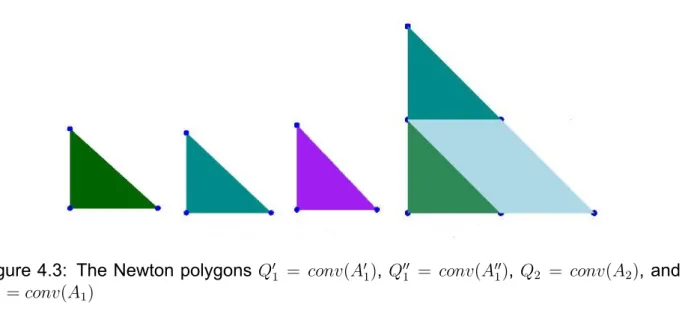
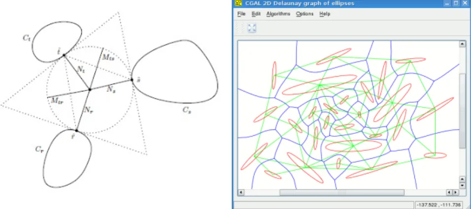
4.1 Left: Voronoi circle for 3 ellipses. Right: An example of a Voronoi diagram for non-intersecting ellipses, and the corresponding Delaunay graph. Both figures reproduced from [45] . . . 54 4.2 The figure is by B. Mourrain using software Mathemagix [92], see also [26] 56 4.3 The Newton polygons Q′1 = conv(A′1), Q1′′ = conv(A′′1), Q2 = conv(A2), and
Q1 = conv(A1) . . . 57
4.4 The Newton polygons Q′1 = conv(A′1), Q′′1 = conv(A′′1), and Q1 = conv(A1) . 58
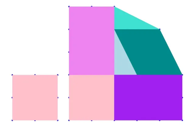
4.5 The Newton polygons Q2 = conv(A2), and Q1+ Q2 = conv(A1+ A2) . . . . 58
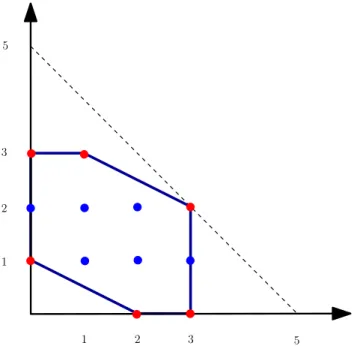
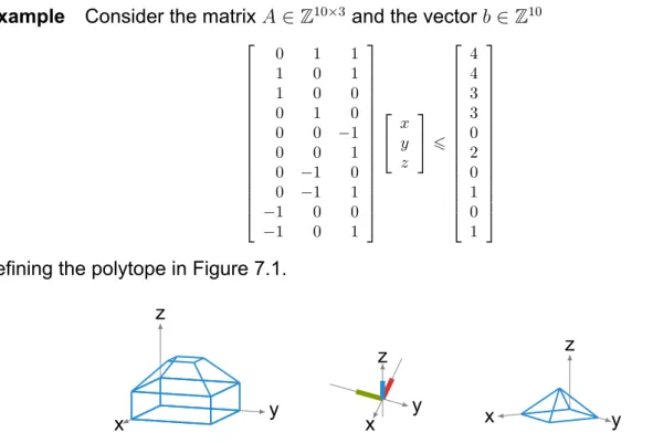
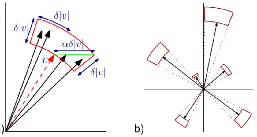
4.6 The discriminant polytope . . . 63 7.1 The polytope defined by System (7.3) and its 2 Minkowski summands. . . . 100 8.1 a) A single cell for the dashed vector v. All vectors in the cell will be deleted.
The distances are shown and the furthest point is in distance αδ|v|. b) After the trim a few cells remain. Every vector in the cells will be deleted and ”represented” by one of the black vectors shown. Notice that the size of each cell depends on the vector that creates it: the shorter the vector the smaller the cell. . . 113 8.2 For every t the returned vector t′ is in distance at most ϵMn+ OP T, where
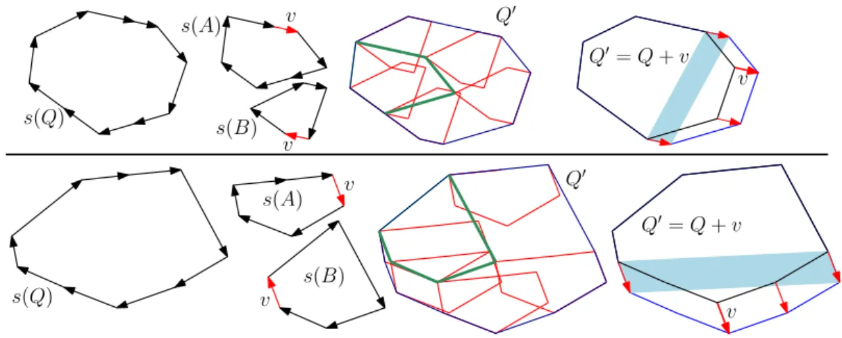
OP T is the optimum distance. . . 117 8.3 Two examples for two polygons Q. Their summands are shown and the red
vector v is the new vector added to fill the gap. At the end, the new polygon
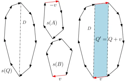
Q′ is Minkowski Sum of the two summands. . . 119 8.4 A worst case example where the vector v is (almost) perpendicular to the
diameter D maximizing the extra volume added. Moreover, D and v have no lattice points thus the interior points added are also maximum (D is not vertical). . . 121 8.5 Experimental results for 2D-SS-opt : a) ϵ = 0.2, b) ϵ = 0.30, c) n = 30,
and d) n = 40. The blue line represents the expected time, the red dots correspond to our experiments. . . 122
8.1 Results for MinkDecomp-µ-approx: input polygon Q, output Q′ (per(Q) > 1000). We measure volume, perimeter and Hausdorff distance and present their mean values. . . 121
This dissertation is submitted for the degree of Doctor of Philosophy at the Department of Informatics and Telecommunications of National and Kapodistrian University of Athens. The research questions were formulated by my supervisor, Prof. Ioannis Z. Emiris, who supported and inspired me in all stages during my PhD. The research was sophisticated, but conducting extensive investigation has allowed me to answer all the questions that we identified. I would like to thank him again for being my supervisor, for the trust he has shown to me from the very first day of our collaboration, helping me to pursue research on topics for which I am truly passionate and achieve those high impact results. His office door was always open and his email available anytime, even late at night or during holidays. Fortunately, both Prof. Evangelos Raptis and Dr. Bernard Mourrain were always helping me, supporting me and encouraging me to continue to the next big step. Thank you for all of the meetings and chats over the years. I would also like to thank Dr. Bernard Mourrain for the funding of my two internships at INRIA Sophia Antipolis - Méditerranée. Many thanks to my tutors Prof. Ilias S. Kotsireas, for his enthusiasm, encouragement and advices and also Prof. Vassilis Zissimopoulos, Prof. Nikolaos Missirlis, and Prof. Michael N. Vrahatis for always being available and willing to answer my queries and guiding me through the project.
I would like to thank my co-authors and tutors Dr. Laurent Busé, Prof. Alicia Dickenstein, Prof. Ioannis Z. Emiris, Dr. Evelyne Hubert, Prof. Gregory Karagiorgos and Prof. Günter Rote, whom I consider myself fortunate to meet, and whose pieces of advise have been priceless.
I would like to thank my co-authors and friends Dr. Eleni Tzanaki, Charilaos Tzovas, Dr. Zafeirakis Zafeirakopoulos for productive collaboration.
I would like to warmly thank my colleagues from the ΕρΓΑ laboratory, Galaad and Aro-math team for their enthusiasm, collaboration, encouragement It was always helpful to share ideas and knowledge about my research. Specially thanks to Evangelos Anagnos-topoulos, Dr. Vissarion Fisikopoulos, Dr. Christos Konaxis, Ioannis Psarros and Dr. Elias Tsigaridas for their advices.
I would like to thank Prof. Dimitris Achlioptas, Dr. Ioannis Chamodrakas, Prof. Ioannis Z. Emiris, Prof. Aggelos Kiayias and Prof. Evangelos Raptis for their trust and tutoring me as assistant.
I would like to thank Antigoni Galanaki and Tatiana Kyrou for helping me with the paper-work.
My sincere gratitude to Prof. Evangelos Raptis, Prof. Korina Rozi and Prof. Dimitrios Varsos for their continuous support and for being my tutors from my early stages until now.
mona, Mr. Charalampos and Ms. Mairy Christoforatos, Manousos Damorakis, Nikos Gri-vokostopoulos, Thalia Ioannou, Ifigeneia Makariti, Zacharias Mpikos, Baggelis Ntaloukas, Charilaos Vougioukas and their families for their continues support and love.
I would like to express my gratitude and appreciation to my big family Karasoulos, Boutidis, Kapogiannis, Xiarchopoulos, Lentzos, Bouloukos, Kalabesios, Ronald and Sara Wildford, Antoni and Basiliki Kourtikaki, Ourania Kalpaxi, Irini and Nikianna Kapogianni, Anastasios and Nikolaos Giannakopoulos, Theodoros Kapogiannis, Christina Kapogianni, Dimitrios and Eleni Karasoulos, Nikolaos and Anna Kapogianni, Panagiota and Sotiria Zoumpou, Christina Lentzou, Nikolaos and Anastasia Lentzos for being by my side and for their love. My parents Nikolaos and Theophanie Karasoulou and my brother Dimitrios Karasoulos deserve a particular note of thanks: your wise advise and kind words have, as always, served me well. Thank you for your infinite support and love. Without you I wouldn’t finish even the first classes of school, of piano Academy, of ballet Academy, of tennis Academy, of .... and most of all of becoming the person that I am today.
My love to my son Nikolaos Lentzos. Thank you for your infinite love and for making my life beautiful. Special thanks to my close family for looking after you while I was doing my research and writing this thesis and for providing funding for the early and the last years of my studies.
Finally, I seize this opportunity to express my love to my husband Konstantinos Lentzos and say a very very big thank you for bearing me in my worst, loving me, encouraging me and supporting me.
I hope you enjoy your reading. Anna Karasoulou
1. INTRODUCTION
In this thesis we worked on problems in the areas of algebraic algorithms, computational geometry and algebraic combinatorics. The first problem is computing the discriminant of a well-constrained sparse polynomial system. The second one is computing the Minkowski decomposition (MinkDecomp) of lattice polytopes and the third one is the problem of Mul-tidimensional Subset Sum (kD-SS) in arbitrary dimension k.
Solving polynomial equations and systems by exploiting the structure and sparseness of them have been studied. The polynomial equations and their respective systems are shown on a various scientific and technological applications . Their solution is the funda-mental problem of Computational Algebra and Computational Algebraic Geometry. Specif-ically, closed formulas for the degree of the sparse (mixed) discriminant and the sparse resultant of polynomial equations have been studied, as well as relationships between them.
Closed formulas when one of the polynomials factors in the context of the theory of sparse elimination using the Newton polytope have been proposed. The main purpose is to facili-tate the computation of the sparse (or mixed) discriminant of a well-constrained polynomial system and to generalize the formula that connects the mixed discriminant with the sparse resultant. The above led to two research papers [39] and [29] .
The paper [39] describes the sparse (or mixed) discriminant and its applications. It also relates it to the sparse resultant of an overconstrained polynomial system, considering the sparse polynomials via the theory of Newton polytopes.
Especially we present our main results relating the mixed discriminant with the sparse resultant of two bivariate Laurent polynomials with fixed support and their toric Jacobian. On our way, we deduced a general multiplicativity formula for the mixed discriminant when one polynomial factors as f = f′·f′′. This formula occurred as a consequence of our main result, Theorem 6.3.3, and generalized known formulas in the homogeneous case to the sparse setting. Furthermore, we obtained a new proof of the bidegree formula for planar mixed discriminants. This work is described in Chapter 4.
In [14] we are given a system of n ⩾ 2 homogeneous polynomials in n variables which is equivariant with respect to the symmetric group of n symbols. We then prove that its resultant can be decomposed into a product of several resultants that are given in terms of some divided differences. As an application, we obtain a decomposition formula for the discriminant of a multivariate homogeneous symmetric polynomial.
Discriminant is a very useful tool, but also very hard to compute. The factorization for-mula that we propose, in the case of symmetric polynomials, reduces the computations significantly. Taking advantage of the polynomial symmetries, the idea is that we gather together the same factors by using combinatorial exponents in the appearing resultants. This work is described in Chapter 5.
poly-nomials with fixed support is proved. The relationship between the sparse (or mixed) discriminant of two bivariate Laurent polynomials with fixed support, with the sparse re-sultant of these polynomials and their toric Jacobian is also given. This helps to obtain a new proof for the bidegree of the discriminant as well as to establish a multiplicativity formula of the mixed discriminant, when one of the polynomials is factorized. This work is described in Chapter 6.
In [36] we present an algorithm for computing all Minkowski Decompositions (MinkDe-comp) of a given convex, integral d-dimensional polytope, using the cone of combinatori-ally equivalent polytopes. An implementation is given in sage. This work is described in Chapter 7.
In [41],[40] we consider the approximation of two NP-hard problems: Minkowski Decom-position (MinkDecomp) of lattice polygons in the plane and the closely related problem of Multidimensional Subset Sum (kD-SS) in arbitrary dimension k. In kD-SS, a multiset S of
k-dimensional vectors is given, along with a target vector t, and one must decide whether there exists a subset of S that sums up to t. We prove, through a gap-preserving reduction from Set Cover that, for general dimension k, the corresponding optimization problem kD-SS-opt is not in APX, although the classic 1D-kD-SS-opt has a PTAS. Our approach relates
kD-SS with the well studied Closest Vector Problem. On the positive side, we present a
O(n3/ϵ2)approximation algorithm for 2D-SS-opt, where n is the cardinality of the multiset
and ϵ > 0 bounds the additive error in terms of some property of the input. We state two variations of this algorithm, which are more suitable for implementation. Employing a reduction of the optimization version of MinkDecomp to 2D-SS-opt we approximate the former: For an input polygon Q and parameter ϵ > 0, we compute summand polygons A and B, where Q′ = A + B is such that some geometric function differs on Q and Q′ by
O(ϵ D), where D is the diameter of Q, or the Hausdorff distance between Q and Q′ is also in O(ϵ D). We conclude with experimental results based on our implementations. This work is described in Chapter 8.
2. BACKGROUND
In this chapter we are giving some definitions and describe some problems that we will refer to in later chapters.
2.1 Preliminaries
A formal definition of the affine space is given below, while Marcel Berger in [7] explains that , ”An affine space is nothing more than a vector space whose origin we try to forget about, by adding translations to the linear maps”.
Definition 2.1.1. An affine space is a set X that admits a free transitive action of a vector
space V . That is, there is a map
X× V → X : (x, v) → x + v,
called translation by the vector v, such that
1. Addition of vectors corresponds to composition of translations, i.e., for all x ∈ X and
u, v ∈ V, x + (u + v) = (x + u) + v.
2. The zero vector acts as the identity, i.e., for all x ∈ X, x + 0 = x.
3. The action is free, i.e., if for a given vector v ∈ V exists a point x ∈ X such that
x + v = x then v = 0.
4. The action is transitive, i.e., for all points x, y ∈ X exists a vector v ∈ V such that
y = x + v.
The dimension of X is the dimension of the vector space of translations, V .
The vector v in Condition 4 that translates the point x to the point y is by Condition 3 unique, and is often written as v = −xy→or as v = y− x. We have in fact a unique map
X× X → V : (x, y) → y − x
such that y = x + (y− x) for all x, y ∈ X. It furthermore satisfies 1. For all x, y, z ∈ X, z − x = (z − y) + (y − x).
2. For all x, y ∈ X and u, v ∈ V, (y + v) − (x + u) = (y − x) + v − u. 3. For all x∈ X, x − x = 0.
Definition 2.1.2. 1. Let a, b be two points ofRn. The set of all x ∈ Rn of the form
x = (1− λ)a + λb, λ ∈ R
is called a line through a and b.
2. A subset M of Rn is called an affine set (affine manifold) if it contains every line
through two point of it. An affine set which contains the origin is a subspace.
Proposition 2.1.3 (Prop 1.1[91]). A nonempty set M is an affine set if and only if M =
a + L, where a∈ M and L is a subspace.
Definition 2.1.4. 1. The subspace L is said to be parallel to the affine set M and it is uniquely defined.
2. The dimension of the subspace L parallel to an affine set M is called the dimension of M . A point a∈ Rn is an affine set of dimension 0, because the subspace parallel
to M = {a} is L = {0}. A line through two points a, b is an affine set of dimension 1, because the subspace parallel to it is the one-dimensional subspace{x = λ(b −
a)|λ ∈ R}. An (n − 1)− dimensional affine set is called a hyperplane or a plane for
short.
Definition 2.1.5. Let x1, . . . , xn be vectors in a real vector space, and let λ1, . . . , λn be
non-negative scalars in R. Then λ1x1 +· · · + λnxn is called a conic combination of the
vectors x1, . . . , xn. If, in addition, λ1 +· · · + λn = 1, then it is a convex combination of
x1, . . . , xn.
Definition 2.1.6. A polyhedron (plur: polyhedra), or polyhedral set inRdis the intersection
of a finite number of half-spaces.
Rather than enumerating a list of n pairs (ai, bi) defining single inequalities, it is usual to
define a n× d matrix A which has the different aias its n line vectors, and a vector b∈ Rn
with the bi, so that it is possible to write the polyhedron as: {x|Ax ⩽ b}
Definition 2.1.7. Let S1, ..., Srbe sets of vectors. We define their Minkowski sum, or vector
sum, as the set of vectors which can be written as the sum of a vector of each set. Namely:
S1+· · · + Sr :={x1+· · · + xr|xi ∈ Si,∀i}.
The Minkowski sum is commutative and associative.
Geometrically, the Minkowski sum is the set of points covered by any translation of one set by a vector in the other one.
Theorem 2.1.8. (Minkowski-Weyl) Any polyhedron is the Minkowski sum of a finitely
gen-erated closed cone and a finitely gengen-erated convex set, and conversely. That is, P is a polyhedron if and only if there are vectors v1, . . . , vn, r1, . . . , rm ofRdsuch that:
As we can see, polyhedra can be described either as a set of inequalities or as a set of generators. These two representations are commonly called H-representation (for half-space) and V-representation (for vertex). If the representation is minimal, the vectors vi
and ri in the V-representation presented here are called vertices and rays. There are
two natural restrictions of this theorem, by excluding either of the conical and convex combinations.
Theorem 2.1.9. (Minkowski-Weyl for cones) Any polyhedral cone is a finitely generated
closed cone, and conversely. That is, P is a polyhedral cone if and only if there are vectors r1, . . . , rm ofRd such that:
P ={µ1r1+· · · + µmrm|µi ⩾ 0}.
Let us now define our main object of study:
Definition 2.1.10. A polytope is a bounded polyhedron.
In other words a polytope is the convex hull of a finite set in Rd. If the finite set is A =
{m1, . . . , ml} ⊂ Rd, then the polytope can be expressed as
Conv(A) = {λ1m1+· · · + λlml : λi ⩾ 0, l
∑
i=1
λi = 1}.
Definition 2.1.11. A lattice polytope is a set of the form Conv(A), where A ⊂ Zd is finite.
That is the convex hull of a set of points with integer coordinates.
Example 2.1.12. If the set of exponent vectors of all monomials of total degree at most
b is Ab = {m ∈ Zd⩾0 : |m| ⩽ b}, then the convex hull of Ab is a polytope (and it is also a
simplex) Qb ={(a1, . . . , ad)∈ Rd : ai ⩾ 0, d ∑ i=1 ai ⩽ d}.
Definition 2.1.13. A simplex is defined to be the convex hull of d + 1 points m1, . . . , mn+1
such that m2− m1, . . . , md+1− m1 are a basis ofRd.
We will now define the faces of a polytope P ⊂ Rd. Let a non zero vector v∈ Rd.
Definition 2.1.14. An affine hyperplane is defined by an equation of the form < m, v >=
−a (the minus sing simplifies certain formulas).
Definition 2.1.15. If ap(v) = − minm∈P(< m, v >), then we call the equation < m, v >=
−aP(v)a supporting hyperplane of P and we call v an inner pointing normal.
The supporting hyperplane has the property that the face of P determined by v is equal to
and P lies in the half-space
P ⊂ {m ∈ Rd:< m, v >⩾ −aP(v)}.
An other approach could be the following: Let P be a polytope and a, x be vectors ofRd,
a ̸= 0 and b a scalar. We say (a, b) is a valid inequality for P , if the inequality < a, x >⩽ b
holds for any point x∈ P .
Definition 2.1.16. For any valid inequality of a polytope, the subset of the polytope of
vectors which are tight for the inequality is called a face of the polytope. That is, the set
F is a face of the polytope P if and only if
F ={x ∈ P | < a, x >= b},
for some valid inequality (a, b) of P . The set of faces of a polytope P is denoted by F (P ). Faces of polytopes can be partially ordered by inclusion, that is, some faces are contained in the others. The partially ordered set of faces of a polytope is called its face lattice.
Definition 2.1.17. Let P be a polytope. The face lattice of the polytope, L(P ), is the
set of faces F (P ) partially ordered by inclusion. That is, for F and G in L(P ), we have
F ⩽ G if and only if F ⊂ G. When the term face lattice is used, it generally implies we are
considering the faces as abstract elements ordered by inclusion, leaving aside geometrical notions.
Definition 2.1.18. If L(P ) is the face lattice of a polytope, a chain S is a subset of L(P )
which is totally ordered, that is, for any distinct F, G∈ S, we have either F ⊂ G or G ⊂ F . The length of a chain is its cardinality minus one. If {F1, . . . , Fn} is a chain, there is an
ordering i1, . . . , in such that Fi1 ⊂ · · · ⊂ Fin .
Theorem 2.1.19. (Face lattices) Let P be a polytope, and L(P ) its face lattice. Then we
have the following:
• The face lattice L(P ) has a unique minimal element, which is the empty set, and a unique maximal element, which is P .
• The face lattice L(P ) is graded, which means that all maximal chains of L(P ) have the same length.
• Let F and G be two faces in L(P ). Then there is a unique maximal face F ∧ G they both contain, and a unique minimal face F ∨ G containing them.
Definition 2.1.20. Let P be a polytope, and F a face of P . The rank of F in the face lattice
L(P )is the length of the longest chain of L(P ) which has empty set and F as minimal and maximal elements respectively.
2.2 Notations
• A set A⊂ Rn is a configuration, if it is contained inZn.
• The configurations A1, . . . , Anare called essential, if the affine dimension of the
lat-tice ZA1+· · · + ZAk equals k− 1 and for all I ⊊ {1, . . . , k} the affine dimension of
the lattice generated by {Ai : i∈ I} is greater or equal than |I|.
• Dense or full configurations are those, who consists of all the lattice points in their convex hull.
2.3 Partitions
Let us now describe throw an example how we arrive to multinomial coefficients through binomial.
• Think of the binomial (104) = 10!
4!(10−4)! as the number of ways to distribute 10 objects
to two recipients such that one receives 4 objects and the other the remaining 6.
• Writing (4, 610) = 4!6!10! instead of just (104) makes explicit the number of objects each recipient receives.
• The multinomial coefficient(3, 4, 310 )= 3!4!3!10! counts the ways to distribute 10 objects to three recipients such that
– the 1st recipient receives 3 objects
– the 2ndrecipient receives 4 objects
– the 3rdrecipient receives 3 objects
In general, the multinomial coefficient is defined as ( n λ1, λ2, . . . , λk ) = n! λ1!λ2! . . . λk!
and equals the number of distributions of n distinct objects to k distinct the recipient i receives exactly λi objects.
Theorem 2.3.1. Multinomial theorem (α1+ α2+· · · + αk)n = ∑ λ1+···+λk=n ( n λ1, . . . , λk ) ∏ 1⩽j⩽k αλj j What is a partition? • λ is a partition of n , denoted as λ⊢ n,
If λ = (λ1, . . . , λk)is a weakly decreasing sequence of nonnegative integers,
λ1 ⩾ · · · ⩾ λk⩾ 0
that sum up to n, i.e. λ1+· · · + λk= n.
• The number of nonzero λi’s is called the length of λ and is denoted as l(λ).
For example 4 has the following five partitions: 4
3 + 1 2 + 2 2 + 1 + 1 1 + 1 + 1 + 1 So (2, 1, 1)⊢ 4 and has length l(2, 1, 1) = 3.
Applying partitions on the variables x1, . . . , xnFor any partition λ = (λ1, . . . , λk)⊢ n, where
k = l(λ),
we construct k blocks of size λ1, . . . , λk in decreasing size order.
Example 2.3.2. The partition (5, 3, 2, 2, 1)⊢ 13 gives
We fill in those blocks with the variables x1, . . . , xn. The λi variables in the block i are
identified by yi and this gives us a ring homomorphism
ρλ : A[x1, . . . , xn]→ A[y1, . . . , yk]
Let us now Count partitions with certain specifications. The following is a fundamental example which leads to the definition of sλ’s How many partitions of 20 have
• one block of size 5 • three blocks of size 4 • three blocks of size 1 ?
Seems that ( 20 1, 1, 1, 4, 4, 4, 5 ) = 20! (1!)3(4!)3(5!)1
has something to do with the answer!
But it is too large to be the correct answer, since the recipients in(1,1,1,204, 4, 4,5)are distinct instead of identical as we want! That is, the multinomial counts the following distributions as different: {17}→recipient 1 {3}→recipient 2 {11}→recipient 3 {2, 5, 6, 10} →recipient 4 {1, 7, 19, 20}→recipient 5 {9, 15, 16, 18}→recipient 6 {4, 8, 12, 13, 14}→recipient 7 {3}→recipient 1 {17}→recipient 2 {11}→recipient 3 {2, 5, 6, 10} →recipient 4 {1, 7, 19, 20}→recipient 5 {9, 15, 16, 18}→recipient 6 {4, 8, 12, 13, 14}→recipient 7
The equivalence principle comes to the rescue: We may arrange the assignment of
• the blocks of size 1 to the first three recipients in any of 3! ways • the blocks of size 4 to the next three recipients in any of 3! ways • the blocks of size 5 to the last recipient in any of 1! ways
and end up with an ”equivalence partition”.
So there are (
20
1, 1, 1, 4, 4, 4, 5 )/
3!3!1! partitions of 20 with blocks of the required description.
In a more formal way a partition is a sequence of weakly decreasing positive integers which is often written as λ = (λ1, . . . , λk). The number k is called the length of λ and will
be denoted by l(λ). When ∑ki=1λi = p we will say such a λ is a partition of p and write
λ⊢ p.
Given a partition λ⊢ n, its associated multinomial coefficient is defined as the integer ( n λ1, λ2, . . . , λl(λ) ) := n! λ1!λ2!· · · λl(λ)! . (2.1)
It counts the number of distributions of n distinct objects to l(λ) distinct recipients such that the recipient i receives exactly λi objects. In this counting, the objects are not ordered
in-side the boxes, but the boxes are ordered. To avoid the count of the permutations between the boxes having the same number of objects we have to divide (2.1) by the number of all these permutations. If sj denotes the number of boxes having exactly j objects, j ∈ [n],
then this number of permutations is equal to ∏nj=1sj!. Thus, for any partition λ ⊢ n we
define the integer
mλ := 1 ∏n j=1sj! ( n λ1, λ2, . . . , λl(λ) ) . (2.2) 2.4 Symmetric polynomials
An n-variable polynomial f (x1,· · · , xn) is called symmetric, if it does not change by any
permutation of its variables. The symmetric n-variable polynomials form a ring. A very common example of such polynomial is the Vandermonde determinant that we analyze below. Symmetric polynomials except for having their own interest, many times reduce a difficult polynomial problem to an easier one by studying it in a symmetric environment. This method is so often used in invariant theory, that is called symmetrization.
Definition 2.4.1. Symmetrization is therefore a process that converts any polynomial in n
variables to a symmetric one in the same number of variables. Thus the symmetrization of a monomial Xa1 1 · · · Xnan is defined as S(Xa1 1 · · · Xnan) = ∑ σ∈Sn Xa1 σ(1)· · · X an σ(n),
where Snstands for the symmetric group.
Example 2.4.2. The symmetrization of X3
1X2 in 3 variables X1, X2, X3 is just
S(X13X2) = X13X2+ X13X3 + X23X3+ X33X1+ X23X1.
Symmetric polynomials are widely used in statistics through bootstrapping processes [69], in chemistry [4], in algebra [1], combinatorics [88], presentation theory of symmetric groups, general linear groups [57], and geometry [60].
For example, a distinguished family of symmetric polynomials called Schur polynomials, that are indexed by combinatorial objects called Young diagrams, describes the charac-ter theory of the symmetric group. The Schur polynomials and their generalizations such as Jack and Macdonald polynomials [68] are related to geometric objects such as sym-metric spaces and flag varieties. They have also found connection with representation theory of super Lie algebras [83, 86]. Besides their connection with representation theory, symmetric functions also have an application to mathematical physics. They are applied in Boson-Femion correspondence which are applied in string theory [58] and integrable systems [76]. There is also an interesting connection to quantum physics: the Jack poly-nomials are the eigenstates of the Hamiltonian of the quantum n-body problem.
Monomial symmetric polynomials
The monomial symmetric polynomial ma is determined by Xa = X1a1· · · Xnan as the sum of
all those obtained by symmetry from Xa. Let us denote d its degree a1+· · · + an.
Consider n-tuples a = (a1, a2, . . . , an) and define the relation ‘‘ ∼ ” between them, which
expresses that one is a permutation of the other. Since ma = mβ, when β is a permutation
of a, one usually considers only those ma for which a1 ⩾ a2 ⩾ . . . ⩾ an and add up to d; in
other words the Young diagrams or partitions of d. Thus one can simply write
mα =
∑
β∼α
Xβ
where b ranges over all distinct permutations of a.
Example 2.4.3. Given a partition a = (2, 1, 1) we get the corresponding symmetric
poly-nomial
m(2,1,1)(X1, X2, X3) = X12X2X3+ X1X22X3+ X1X2X32.
The monomial symmetric polynomials form a basis of the infinite dimensional vector space of symmetric polynomials and as a consequence every symmetric polynomial F can be written as a linear combination of them. To this point, it suffices to separate the different types of monomials occurring in F . In particular, if F has integer coefficients, then so will the linear combination.
Power sum symmetric polynomials
For each integer k ⩾ 0, the monomial symmetric polynomial m(k,0,...,0)(X1, . . . , Xn) is of
special interest. It is called the k-th power sum symmetric polynomial and is denoted as
sk(X1, . . . , Xn), so sk(X1, . . . , Xn) = X1k+ X k 2 +· · · + X k n
Any symmetric polynomial in X1, . . . , Xncan be expressed as a polynomial expression with
rational coefficients in the power sum symmetric polynomials s1(X1, . . . , Xn), . . . , sn(X1, . . . , Xn).
Remark 2.4.4. The ring of symmetric polynomials with coefficients in a fieldK of
charac-teristic zero is equal to the polynomial ringK[s1, . . . , sn].
Symmetric polynomials
Definition 2.4.5. Let X1, . . . , Xn be indeterminates over Z, where n is a positive integer.
The monic polynomial g∈ Z[X1, . . . , Xn][X]having roots X1, . . . , Xn expands as
g(X) = n ∏ i=1 (X − Xi) = ∑ j∈Z (−1)jejXn−j, (2.3)
whose coefficients are, up to sign, the elementary symmetric polynomials of X1, . . . , Xn,
ej = ej(X1, . . . , Xn) = ∑ 1⩽i1⩽...⩽ij⩽n j ∏ k=1 Xik, j ⩾ 0
and ej = 0, for j < 0 and j > n, e0 = 1.
An equivalent definition of elementary symmetric polynomials is the following: The
ele-mentary symmetric polynomials are particular cases of monomial symmetric polynomials.
For 0⩽ k ⩽ n, we define ek(X1, . . . , Xn) = mα(X1, . . . , Xn), where a = (1, . . . , 1 | {z } k , 0, . . . , 0 | {z } n−k ).
If now we give to the ring of polynomials in X1, . . . , XnoverZ a name, R = Z[X1, . . . , Xn],
then the symmetric group Snof all permutations of{1, . . . , n} acts on R. That is a
permu-tation σ∈ Sn gives rise to an automorphism aσ : S→ S, defined as
aσ(g(X1, . . . , Xn)) = g(Xσ(1), . . . , Xσ(n)), σ ∈ Sn, f ∈ Z[X1, . . . , Xn].
A polynomial F ∈ R is called a symmetric polynomial if for all σ ∈ Sn
F (X1, . . . , Xn) = F (Xσ(1), . . . , Xσ(n)).
R0 ={Sn− invariant polynomials in R}.
The product form (2.3) shows that the ejare invariant under the action and henceZ[e1, . . . , en]⊂
R0. In fact it is an equality.
Theorem 2.4.6. (Fundamental Theorem of Symmetric Polynomials). The subring of
poly-nomials inZ[X1, . . . , Xn]that are fixed under the action of SnisZ[e1, . . . , en].
This theorem is also true for any ℜ commutative ring. Then every symmetric polynomial inℜ[X1, . . . , Xn]is a polynomial in the elementary symmetric polynomials in a unique way.
In other words if F (X1, . . . , Xn) is symmetric, then there exists a unique polynomial q ∈
ℜ[X1, . . . , Xn]such that q(e1, . . . , en) = F (X1, . . . , Xn). The discriminant of g in (2.3) is ∆(g) = ∏ 1⩽i<j⩽n (Xi− Xj)2.
It is invariant under Sn and lies in the coefficient field of g. Expressing ∆ in the terms of
the ej is not so easy, although the proof of the Fundamental Theorem of Symmetric
Poly-nomials shows an algorithm which determines the expression for a given Sn−invariant
polynomial in terms of the elementary ones. For example, in the case n = 2, the dis-criminant of g can be written in the terms of the elementary symmetric functions of the Xi
as
∆(g) = (X1− X2)2 = X12− 2X1X2+ X22 = (X1+ X2)2− 4X1X2 = e21− 4e2.
The square root of the discriminant √∆ = ∏1⩽i<j⩽n(Xi − Xj) is not symmetric. In fact
√
∆ is fixed by An but not by Sn, where An stands for the subset of Sn that formed by
even permutations and it is a group that called the alternating group. This polynomial, that we usually denote by V (X1, . . . , Xn)is the value of the Vandermonde determinant of the
matrix: 1 X1 X12 · · · X d−1 1 1 X2 X22 · · · X d−1 2 .. . ... ... ... 1 Xn Xn2 · · · Xnd−1 .
Complete homogeneous symmetric polynomials
A symmetric polynomial is homogeneous in the variables X1, . . . , Xn of degree d, if every
monomial in it has total degree d. The total degree d of a monomial cXa1
1 , . . . , Xnan is the
sum of the exponents, that is d = a1+· · · + an.
For each nonnegative integer k, the complete homogeneous symmetric polynomial hk(X1, . . . , Xn)
is the sum of all distinct monomials of degree k in the variables X1, . . . , Xn. For instance
h3(X1, X2, X3) = = X13+ X12X2+ X12X3+ X1X22+ X1X2X3+ X1X32+ X 3 2 + X 2 2X3 + X2X32+ X 3 3.
![Figure 4.2: The figure is by B. Mourrain using software Mathemagix [92], see also [26]](https://thumb-eu.123doks.com/thumbv2/123doknet/14670646.741575/57.892.296.567.159.486/figure-figure-b-mourrain-using-software-mathemagix.webp)