Finite volume simulation of cavitating flows

HAL Id: hal-00139597

https://hal.archives-ouvertes.fr/hal-00139597

HAL is a multi-disciplinary open access archive for the deposit and dissemination of sci-entific research documents, whether they are pub-lished or not. The documents may come from

L’archive ouverte pluridisciplinaire HAL, est destinée au dépôt et à la diffusion de documents scientifiques de niveau recherche, publiés ou non, émanant des établissements d’enseignement et de

Finite volume simulation of cavitating flows

Thomas Barberon, Philippe Helluy

To cite this version:

Thomas Barberon, Philippe Helluy. Finite volume simulation of cavitating flows. Computers and Fluids, Elsevier, 2005, 34 (7), pp.832-858. �hal-00139597�

Finite Volume simulation of cavitating flows

Thomas Barberon, Philippe Helluy

ISITV, Laboratoire MNC, BP 56, 83162 La Valette, France

Abstract

We propose a numerical method adapted to the modelling of phase transitions in compressible fluid flows. Pressure laws taking into account phase transitions are complex and lead to difficulties such as the non-uniqueness of entropy solutions. In order to avoid these difficulties, we propose a projection finite volume scheme. This scheme is based on a Riemann solver with a simpler pressure law and an entropy maximization procedure that enables us to recover the original complex pressure law. Several numerical experiments are presented that validate this approach.

Key words: cavitation, Godunov scheme, two-phase compressible flow

1 Introduction

This work is devoted to the numerical modelling of phase transition in com-pressible fluid flows. We focus on the liquid-vapor phase transition also called cavitation. For this we consider the Euler system for an inviscid and com-pressible fluid together with a pressure law that ensures the hyperbolicity of the Euler system. This system has been extensively studied, both theoretically and numerically. Standard textbooks exist now on this subject [14], [29], [30]. The global existence and uniqueness of a solution to this system, for general initial conditions, is still an open question.

On the other hand, the Riemann problem, which consists of finding a one dimensional solution for a particular initial condition made of two constant states, is well understood. It is known that a supplementary dissipation cri-terion must be added in order to recover uniqueness. This cricri-terion can take several forms. The most classical criteria are:

(1) The Lax entropy criterion: any Lax entropy should increase in shocks. Email address: [email protected] (Philippe Helluy).

(2) The Lax characteristic criterion: a shock of the i−th family should be crossed by the i−th characteristics coming from the two sides of the shock.

(3) The vanishing viscosity criterion: the solution should be the limit of solu-tions of the Euler system perturbed by a supplementary viscosity term. (4) Liu has proposed in [23] a stricter criterion than the Lax entropy criterion

(1). It requires that the entropy increases along the entire shock curve joining the left and the right states of the shock and not only globally. In the case of a simple pressure law, such as the perfect gas law, it appears that these four criteria are equivalent and ensure existence and uniqueness of the solution. But for more complex laws used for the modelling of phase transitions, the situation is not so clear. In some configurations, one can indeed find several solutions satisfying criteria (1)-(4), even if the pressure law ensures the hyperbolicity of the system. A very detailed study of these topics can be found in the important paper of Menikoff and Plohr [24]. Detailed examples can also be found in the thesis of Jaouen [18]. In this reference a proof of non-uniqueness is also given in the case of a simplified phase transition pressure law.

It can also happen that none of the criteria (2)-(4) are physically relevant. For instance, Hayes and LeFloch study in [15] the effect of a vanishing third order perturbation to the initial hyperbolic system. This term permits to model capillarity near the critical point. They show that in general the limit shock solutions do not satisfy criteria 2-4. Special schemes have to be designed in order to approximate these non-classical shocks [21].

For classical pressure laws, the Riemann problem solution is made up of sev-eral constant states separated by shock waves, simple waves and one contact discontinuity. Phase transition pressure laws may present pathologies such as slope discontinuities, lack of convexity of the isentropes or of the Hugoniot curves in the (τ, p) plane. These pathologies lead to a more complex resolu-tion of the Riemann problem. One has to take into account the possibility of composite waves. This subject is studied in the paper of Menikoff and Plohr [24]. Classical references about the Riemann problem for arbitrary fluids are also [5], [33], [32]. Thus, even if the Riemann problem is still uniquely solvable, it is difficult to practically implement it in a Godunov type scheme.

Several numerical methods have been proposed to solve the Euler system with complex pressure laws. Some methods rely on approximate Riemann solvers [13], [18], [2]. These methods must be carefully employed because even if the scheme is entropic it may converge towards wrong solutions due to the non-uniqueness of the solution. This possible behavior is illustrated in [18], where an entropic Godunov-type scheme converges to different solutions according to the CFL number.

In this paper we focus on special pressure laws. We suppose that the pressure law is obtained from a physical entropy maximization with respect to supple-mentary (intermediate) variables. This is not a restriction for phase transitions because it is exactly the way the liquid-vapor mixture is classically modelled [6]. We then use this representation in order to design a finite volume scheme, which we first described in [17] and [3]. Each time-step of this scheme is made up of two sub-steps:

(1) A standard Godunov resolution taking into account the intermediate vari-ables. In this step, the intermediate variables are simply convected with the fluid. It appears that the associated Riemann problem is easier to solve than the original one. Indeed, the relaxed pressure law with inter-mediate variables has no pathology. This step is entropic because we use an exact Riemann solver.

(2) Then, the conservative variables are kept for the next time step. The pressure is updated by maximizing the physical entropy with respect to the intermediate variables. This amounts to projecting the relaxed pressure law towards the real pressure law. This step is also entropic by construction.

The paper is thus organized as follows.

Following this Introduction, the second section is devoted to a presentation of a simple mathematical framework for the modelling of phase transition. We consider the flow of a compressible liquid which is subject to phase transition. The idea is to add to the initial Euler system a convection equation with a relaxation source term for a supplementary vector Y (t, x) called the fractions vector, which plays the role of the intermediate variables. The complex initial pressure law is replaced by a simpler relaxed pressure law which depends on density, internal energy and the fractions. We associate an entropy to this simpler pressure law. We then define the equilibrium fractions Yeq by an

op-timization of the entropy with respect to Y . We suppose that the complex pressure law is recovered by replacing Y with Yeq in the relaxed pressure law.

The idea of replacing a complex pressure law by a simpler one together with a relaxation procedure was first proposed by Coquel and Perthame in [9]. Relaxation source terms are extensively used in the seven-equation model of Abgrall and Saurel in [26]. This idea has also been exploited in [7], [20], [11] for the modelling of two-phase flows without phase transition. Even when the two phases are supposed to be immiscible, it is necessary, for numerical reasons, to define a mixture pressure law. This mixture pressure law is obtained by imposing pressure equilibrium between the two phases and can be quite complicated. Thus, in order to use an exact Riemann solver, it is interesting to relax the pressure law. This is done in [7], [20] by solving a supplementary convection equation for the volume fraction of one fluid. At the end of each

time step, this volume fraction is modified in order to recover the pressure equilibrium.

We then apply the above mathematical framework to a physical model of vapor-liquid mixture. We consider two fluids which are supposed to be immis-cible on a small scale. The behavior of each fluid is entirely described by its specific entropy which is a function of the specific volume and of the internal energy. Using the physical fact that the entropy is an extensive variable, it is then possible to get in a unique manner the mixture entropy, function of the specific volume, the internal energy and the fractions. Then the second prin-ciple of thermodynamics tells us that the equilibrium fractions must realize a maximum of the mixture entropy. This maximization process enables us to reconstruct a physically coherent equilibrium pressure law.

In the third section of the paper, we apply this theory to a mixture of two phases satisfying the stiffened gas equation of state. In order to have simpler computations, we suppose that thermal equilibrium always hold. In this way, it is possible to eliminate the energy fraction from the unknowns. Then, an important feature is that the resulting relaxed mixture pressure law is still a stiffened gas law even though the equilibrium pressure law is no longer one. If the stiffened gases are perfect gases, the computations are even simpler. The fourth section is devoted to the study of the Riemann problem associ-ated to the pressure law of the previous section. We briefly explain how it is possible to construct several entropy solutions to the Riemann problem. This construction is not original and is entirely contained in the thesis of Jaouen [18]. It is used in the fifth section to validate the numerical scheme.

In the fifth section, we present the projection scheme. The description is very simple. Each time step of the finite volume scheme is made up of two stages. In the first stage, a simple Godunov scheme is employed. Thus, in this stage, the phase transition is not taken into account. Because the pressure law is simplified, it is possible to use an exact Riemann solver and to have the correct entropy dissipation. In the second stage, the fraction vector is modified in such a way as to maximize the entropy of the mixture in each cell. This stage is conservative, because the density, velocity and energy are not modified. It is also entropy dissipative by construction.

We then illustrate the projection scheme on several 1D numerical experiments. In particular, we verify that it is able to reproduce the physical entropy solution constructed in Section 4. It is important to notice here that the numerical solution does not depend on the CFL number. We explain the good behavior of the projection scheme by the fact that the production of entropy occurs not only in the Godunov step but also because of the phase transition. This is important because a global entropy production is not sufficient.

Section 6 is then devoted to a 2D simulation in order to illustrate the ability of our scheme to deal with physical configurations. This test is very similar to the one proposed by Butler, Cocchi and Saurel in [28]. The goal is to compute the flow around a fast projectile diving into water at a velocity of 1000 m/s. A strong pressure loss appears in the wake of the projectile, triggering the growth of a cavitation pocket. We are able to qualitatively reproduce this phenomenon.

The paper ends with a conclusion (Section 7).

2 Mathematical models for phase transition

This section is devoted to a presentation of a simple mathematical framework for the modelling of phase transition. We consider the two-phase vapor-liquid mixture as a single compressible medium with (in 1D) density ρ(t, x), velocity u(t, x), internal energy ε(t, x) and pressure p(t, x), all depending on the time variable t and the space variable x. Conservation of mass, momentum and energy and Newton’s law for inviscid flow lead to the three Euler equations:

ρt+ (ρu)x= 0,

(ρu)t+ (ρu2+ p)x= 0, (1)

(ρε + ρu2/2)t+ ((ρε + ρu2/2 + p)u)x= 0.

If the flow is not too fast, i.e. if the equilibrium between the liquid and its vapor is achieved for all (t, x), the pressure of the whole mixture depends only on the density ρ and the internal energy ε. We shall write

p = peq(ρ, ε). (2)

This equilibrium pressure law is generally quite complex, and more important, leads to unclassical behaviors of the solutions: non-uniqueness of the entropy solution, composite waves. We insist on the fact that this has nothing to do with a defect of hyperbolicity. Phase transition pressure laws naturally ensure the hyperbolicity. For example, the Van der Waals pressure law is a bad model of phase transition and has to be modified by Maxwell’s construction in order to eliminate the elliptic region, and the modified law ensures hyperbolicity [6]. We propose in this section a more general model, in which we no longer sup-pose the equilibrium of the two-phase mixture. We have thus to introduce supplementary variables and the pressure will also depend on these variables.

This pressure law will be called the relaxed pressure law. Because the resulting model is out of equilibrium, we shall denote it as the metastable model. Of course we will also have to return to the equilibrium pressure law. This will be done by a projection method. Although it would be interesting to account for the dynamics of the phase transition, we do not deal with this problem here and just use the metastable model in order to compute the equilibrium model.

2.1 A generalized metastable model

A supplementary vector of variables, called the fractions vector Y (t, x) is used in order to model vaporization. The components Yi_{, 1 ≤ i ≤ N satisfy}

0 ≤ Yi ≤1. (3)

Usually, the fraction vector Y will have three components that are the mass, volume and energy fractions of the vapor in the mixture. But simpler models will only consider one or two fractions. We suppose that when the fluid is pure liquid, Yi _{= 0, and when the fluid is pure vapor, Y}i _{= 1. When no phase}

transition occurs, there is no transfer between the liquid and its vapor, thus we also have perfect convection of the fractions:

Yt+ uYx = 0. (4)

Using the mass conservation law, the convection of the fractions can be written in an equivalent conservative form

(ρY )t+ (ρuY )x = 0. (5)

We have to close these equations with a pressure law

p = p(ρ, ε, Y ). (6) When equations (1), (5) and (6) are considered, we will speak of the metastable model. Indeed, in this model the fractions are simply convected in the flow, and thus, there is no transfer between the two phases.

It is well known that the solution of model (1), (5), (6) is not unique and that a supplementary condition has to be added to restrict the set of solutions. For a simple pressure law, this can be an entropy growth criterion. But it can be necessary to envisage other criteria as described in the Introduction. With τ = 1/ρ, an entropy is a concave function s = s(τ, ε, Y ), solution of the first order PDE

Generally, one can find several entropies. Defining the temperature by

T = 1/sε, (8)

we recover the relation

T ds = dε + pdτ + sYdY. (9)

Thus, choosing an entropy amounts to choosing the temperature scale. It also permits us to recover the pressure law by

p = T sτ. (10)

A given entropy is called a complete equation of state (see [24]) because it permits us to recover the pressure law (10) and the caloric law (8). When one studies the dynamic behavior of a compressible fluid, an incomplete equation of state, the pressure law, is sufficient. But if one wishes to model a ther-modynamic feature such as the phase transition, it is necessary to fix the temperature scale and thus a complete equation of state is required. In the sequel, we then suppose that one particular entropy has been selected. The construction of the mixture entropy from the entropies of the two phases and from physical considerations is described below.

Simple computations show that a regular solution of system (1), (5), (6) sa-tisfies

st+ usx = 0, (11)

which can be cast into a conservative form

(ρs)t+ (ρus)x = 0. (12)

When dealing with discontinuous solutions, the latter has to be replaced by an inequality, in the sense of distributions, in order to recover uniqueness

(ρs)t+ (ρus)x≥0. (13)

Recall that the concavity of s with respect to (τ, ε, Y ) is equivalent to the convexity of the quantity U = −ρs with respect to the conservative variables (ρ, ρu, ρε + ρu2_{/2, ρY ) (see [14], [10]). This implies that U = −ρs is indeed a}

Lax entropy of the metastable model.

2.2 Entropy compatible transition models

In order to take phase transition into account, we add a source term to equation (5)

Equations (1), (6) together with (14) will be referred to as the cavitation or transition model. In the case where the phase transition is infinitely fast, we will always have

Y = Yeq(ρ, ε), (15)

because the repartition of liquid and vapor is completely determined by the phase diagram. We require that the resulting pressure law is exactly the equi-librium pressure law (2)

p = p(ρ, ε, Yeq(ρ, ε)) = peq(ρ, ε). (16)

It is then natural to consider, as in [9], a relaxation source term of the form µ = λ(Yeq(ρ, ε) − Y ), (17)

and then to let λ → ∞.

Suppose then that the equilibrium fractions Yeq are defined by

s(ρ, ε, Yeq(ρ, ε)) = max

Y ∈Qs(ρ, ε, Y ), (18)

where Q is the set of admissible parameters.

It is then interesting to compute the production of entropy along the stream-lines of the flow, when all the unknowns are regular. Using (10) and (8), this production is given by ˙s := st+ usx = sτ(τt+ uτx) + sε(εt+ uεx) + ∇Ys · (Yt+ uYx) = −p T ρ2(ρt+ uρx) + 1 T(εt+ uεx) + ∇Ys · (Yt+ uYx). (19)

But on the other hand, a regular solution of the Euler system (1) also satisfies ρt+ uρx+ ρux= 0, ut+ uux+ px ρ = 0, εt+ uεx+ p ρux = 0, (20)

thus, the production of entropy can be simplified and thanks to the concavity of s, for the cavitation model (equations (1), (6), (14) and (17)) we have also

st+ usx = ∇Ys · (Yt+ uYx) ,

= λ∇Ys · (Yeq−Y )

≥λ (s(Yeq) − s(Y ))

≥0,

The entropy condition is thus reinforced when compared to the metastable model (equations (1), (5) and (6)) because the production of entropy occurs not only in shocks but also as a result of the phase transition.

2.3 Mixture entropy

We will now apply the above mathematical framework to a physical model of vapor-liquid mixture. We consider two fluids, or phases, that are supposed to be immiscible at a small scale. As already pointed out, the behavior of each phase is entirely described by its specific entropy function. Using the physical fact that the entropy is an extensive variable, it is then possible to get in a unique manner the mixture entropy, function of the specific volume, the internal energy and the fractions.

Let us now detail the computation of the mixture entropy. Let V be a small volume occupied by the two fluids which we index by (1) and (2). The fluid (i) fills a volume Vi in V and we have V1+ V2 = V , because the two fluids are

immiscible on a small scale. The volume fraction of fluid (i) is defined by αi =

Vi

V . (22)

On a small scale, the density of fluid (i) is ρ_i. But because fluid (i) does not fill all the volume V , the apparent density, on a large scale, is ρi = αiρi. The

mixture density is ρ = ρ1 + ρ2. The mass fraction of fluid (i) is defined by

yi =

ρi

ρ. (23)

On the other hand, the large scale internal energy is linked to the small scale internal energy by εi = yiεi. It is then possible to define the energy fraction

of fluid (i) by

zi =

εi

ε. (24)

We also set α = α1, y = y1, z = z1 (and thus α2 = 1−α, y2 = 1−y, z2 = 1−z).

Now, the thermodynamic behavior of each fluid is completely determined by its specific, i.e. per unit mass, entropy function

si = si(τi, εi), (25)

where we have defined the specific volume τ by τ = 1/ρ. Indeed, the caloric law, which expresses the temperature Ti of fluid (i), is recovered by

1 Ti

= ∂si ∂εi

and the pressure law is given by pi Ti = ∂si ∂τi . (27)

Then according to the second principle of thermodynamics, the entropy is an additive (extensive) variable. Setting Y = (α, y, z)T_{, this means that the}

mixture specific entropy is necessarily given by

s(τ, ε, Y ) = ys1(τ1, ε1) + (1 − y)s2(τ2, ε2), (28) or s(τ, ε, Y ) = ys1( α yτ, z yε) + (1 − y)s2( 1 − α 1 − yτ, 1 − z 1 − yε). (29) It can be checked that s is concave with respect to (τ, ε, Y ), thanks to the concavity of si.

Then the second principle of thermodynamics tells us that the equilibrium fractions must realize a maximum of the mixture entropy

s(τ, ε, Yeq) = max

0≤Y ≤1s(τ, ε, Y ). (30)

There is also a more mathematical interpretation of the equilibrium entropy as the inf-convolution of the entropies of the two phases. It is described in [16]. An important fact is that the maximum in (30) is under the constraint that all the fractions are between 0 and 1. Thus it does not necessarily imply that the gradient of the entropy with respect to the fractions is zero. If the maximum is attained in the interior of the constraint set, i.e. if each component of Yeq is

in the open interval ]0, 1[, it is characterized by ∂s ∂α = τ ( p1 T1 − p2 T2 ) = 0, (31) ∂s ∂z = ε(1/T1−1/T2) = 0, (32) ∂s ∂y = −(µ1/T1−µ2/T2) = 0, (33) where µi is the specific Gibbs function of fluid (i), also called the fluid (i)

chemical potential, defined by

µ = ε + pτ − T s. (34) We recover the fact that at equilibrium, the pressures, temperatures and chem-ical potentials of the two phases are identchem-ical. On the other hand, the maximum can be attained on the boundary of the constraint set. In this case, only one phase is stable.

The mixture entropy (29) also defines a mixture pressure law and a caloric law out of equilibrium:

p = T sτ = T (αp1/T1+ (1 − α)p2/T2), (35) 1 T = z T1 + 1 − z T2 . (36)

3 A simple pressure law for phase transition

3.1 Mixtures of stiffened gases

In this section, we apply the theory to a mixture of two phases satisfying the stiffened gas equation of state. In order to have simpler computations, we will suppose that thermal equilibrium always holds. In this way, it is possible to eliminate the energy fraction from the unknowns. Then, an important feature is that the resulting relaxed mixture pressure law is still a stiffened gas law even though the equilibrium pressure law is no longer one. The interest of the stiffened gas law is that the associated Riemann problem is easy to solve exactly and this fact will be exploited in the numerical method below.

We consider a simple case where the entropies of the two fluids are those of a stiffened gas

si = Ciln((εi−Qi−πiτi)τγii−1) + s0i. (37)

The law is characterized by several physical constants. The parameter Ci is

the specific heat of fluid i. The parameter Qi can be interpreted as a heat of

formation. The parameter πi has the dimension of a pressure and −πi is the

minimal pressure for which the sound speed of fluid i vanishes This aspect is detailed in [4]. The parameter γi is the adiabatic exponents and s0i is the

reference entropy of phase i. All these constants can be fitted to experimental data: see [8] and below. The caloric law and the pressure law are given by

CiTi = εi−Qi−πiτi,

pi = (γi−1)ρi(εi −Qi) − γiπi.

(38) We also have

pi+ πi = (γi−1)ρiCiTi. (39)

A further simplification is to suppose equilibrium of temperatures, T = T1 =

C = yC1 + (1 − y)C2, (40) Q = yQ1+ (1 − y)Q2, (41) π = απ1+ (1 − α)π2, (42) γ = yγ1C1 + (1 − y)γ2C2 yC1 + (1 − y)C2 , (43) we obtain p = (γ − 1)ρCT − π, (44) CT = ε − Q − π ρ. (45)

In this way, the mixture behaves as a stiffened gas. It must be noted that the elimination of the energy fraction z is necessary in order that the mixture behaves like a stiffened gas. However, if one eliminates the volume fraction α by imposing the pressure equilibrium, then the pressure law is no longer a stiffened gas law, except when the two phases satisfy πi = 0, i.e. when they

are perfect gases.

Applying (29) and the above computations (37-45), the entropy of the mixture of stiffened gases is s(τ, ε, α, y) = C ln(ε − Q − πτ ) − C ln C + (γ − 1) ln τ + ln   Ã α y !yC₁(γ₁−1)Ã 1 − α 1 − y !(1−y)C₂(γ₂−1) + Ky. (46)

3.2 Mixtures of perfect gases

Here, we again simplify the model by supposing that the two phases are perfect gases. In this case, it is also convenient to eliminate the volume fraction in the model. The only remaining fraction is then the mass fraction y. The mixture pressure law is still a perfect gas law. If one optimizes the mixture entropy with respect to y we recover the phase transition model studied by Jaouen in [18].

The simplified entropies are given by (we have set Γ = γ − 1)

si = ln(εiτΓii ). (47)

The thermal equilibrium is expressed by

And then the pressure equilibrium gives p1 = Γ1ε1/τ1 = p2 = Γ2ε2/τ2, Γ1 y α = Γ2 1 − y 1 − α. (49)

We can thus express α as a function of y. α = Γ1y

Γ , 1 − α =

Γ2(1 − y)

Γ , (50)

with

Γ = Γ(y) = yΓ1+ (1 − y)Γ2. (51)

Finally, again using (29) the mixture entropy is s = y ln Ã ε µΓ 1 Γ τ ¶Γ1! + (1 − y) ln Ã ε µΓ 2 Γτ ¶Γ2! , = ln ε + Γ ln τ + yΓ1ln Γ1+ (1 − y)Γ2ln Γ2−Γ ln Γ. (52)

The fraction vector Y is in this case reduced to the mass fraction y. Out of equilibrium, the mixture is still a perfect gas for we have ∂s

∂ε = 1 T = 1 ε and ∂s ∂τ = p T = Γ(y) τ .

In the sequel, we suppose that Γ1 > Γ2, i.e. the phase (1) is less dense than

the phase (2)). The derivative of s with respect to y is ∂s

∂y = (Γ1−Γ2) ln τ + Γ1ln Γ1−Γ2ln Γ2 −(Γ1−Γ2) ln Γ − (Γ1−Γ2).

(53)

The saturation curve for this phase transition model is defined by ∂s/∂y = 0. We find that the saturation curve is, in the plane (T, p), a straight line with equation T p = exp(1) Ã ΓΓ11 ΓΓ2 2 ! 1 Γ2−Γ1 = G. (54)

Maximizing s with respect to y under the constraints 0 ≤ y ≤ 1 permits to recover the equilibrium pressure law

             peq(τ, ε) = Γ2ε/τ if τ ≤ τ2, peq(τ, ε) = _G1ε if τ2 ≤τ ≤ τ1, peq(τ, ε) = Γ1ε/τ if τ ≥ τ1, (55) with τi = GΓi. (56)

4 Construction of an analytical solution

In this part, we consider the Euler system (1) and the pressure law (55). The Euler system can also be written

Wt+ F (W )x = 0, (57)

with W = (ρ, ρu, ρε + ρu2_/2)T_{. We will also use a privileged set of}

non-conservative variables that we denote V = (τ, u, p)T_{. We recall briefly how}

it is possible to construct several entropy solutions to the Riemann problem that consists of finding solutions to (1) when the initial condition is

W (0, x) =      Wl if x < 0, Wr if x > 0. (58)

We will compute precisely the correct entropy solution, that is the limit of viscosity solutions or that satisfies the Liu entropy condition. This analytical solution will be used to validate our scheme in Section 5.3.

4.1 A simple entropy shock solution

We only consider solutions made of one or several shock waves. A shock solu-tion of velocity σ has the form

W (t, x) =      WL if x/t < σ, WR if x/t > σ. (59)

The Rankine-Hugoniot shock conditions must be satisfied. Denoting [φ] the jump of the quantity φ across the discontinuity ([φ] = φR−φL), they can be

written as σ[W ] = [F (W )] or              σ [ρ] = [ρu] , σ [ρu] =hρu2+ pi, σ " ρε + ρu 2 2 # = "Ã ρε + ρu 2 2 + p ! u # . (60)

Defining the Lagrangian velocity of the shock by

▲ ▲ ▲ ❊ ❊ ❊ τ p τ₂ τ₁ (τR,pR) (τ1,p1) (1)+(2) (1) (2) ”gas” ”liquid” saturation zone o Rayleigh line (τ ,p) o o o o u p o o o (uR,pR) (uL,pL) (u∗_,p∗₎ 1-shock locus of origin wR 3-shock locus of origin wL 1-shock locus of origin w1 o (u,p) Rayleigh line (u₁,p₁) (τL,pL)

Fig. 1. Non-uniqueness of the Riemann problem we have equivalently                    j2 = −[p] [τ ], j = [p] [u], [ε] + 1 2[τ ] (pL+ pR) = 0. (62)

If j > 0, we are in the case of a 3-shock, if j < 0, it is a 1-shock. The case j = 0 corresponds to a contact discontinuity. If VR = (τR, uR, pR) is fixed and

if j > 0, the three equations in (62) define a curve, called the Hugoniot curve, in the space (τ, u, p) of all the states VL= (τL, uL, pL) that can be connected to

VR by a 3-shock. This curve can parameterized by τ or j for instance: details

can be found in [14], [18].

4.2 Non-uniqueness of the entropy solution

We first construct an entropy solution made of a single shock wave. For this, we choose an arbitrary state VR= (τR, 0, pR) in the light phase, thus τR> τ1.

In the numerical experiments, we shall use, as in [18], τR= 1.3 and pR = 0.1.

We choose also Γ1 = 0.6 and Γ2 = 0.5. This allows the computation of τ1 and

τ2 (according to (56)). The numerical values are summed up in Table 1.

We build the Hugoniot curve of origin VR. As represented in Figure 1, the

projection of this curve on the plane (τ, p) is not convex at the point defined by τ = τ1.

The left state VLis chosen on the Hugoniot curve, inside the saturation region,

thus τ2 < τL < τ1. For the numerics, we take, as in Jaouen [18], τL = 0.92.

Hugoniot curve      p(τ ) = pR(Γ_{Γ1(τ −τR)+2Γ1}1+2)τR−Γ1τ if τ1 ≤τ, p(τ ) = pR(Γ1+2)τR−Γ1τ_{Γ1(τ −τR)+2τ1} if τ2 ≤τ ≤ τ1. (63)

Then, pL = p(τL). The velocity uL, the Lagrangian velocity jL, and thus the

shock velocity σ along the Hugoniot curve are easily deduced from (62). In this way, we have constructed a shock solution of the Riemann problem. It can be checked that it is entropic and satisfies the Lax characteristic condition. But this solution is not physical, i.e. has no viscous profile. Details can be found in [18]. We just mention that along the Hugoniot curve, the variation of entropy is given by

T ds = 1 2[τ ]

2

d³j2´. (64) According to (62), j2 _{is also the opposite of the slope of the Rayleigh line,}

which is the line joining wR and w) in the plane (τ, p). It can then be seen

on Figure 1, that the entropy is increasing between wR and w1 and decreasing

between w1 and w. The production of entropy in the first part of the Hugoniot

curve is bigger than the decrease of the entropy in the second part. Thus the shock is globally entropic but does not satisfy the Liu entropy condition. It is indeed possible to construct another solution, which is the only physical solution. We keep the first part of the Hugoniot curve, outside the saturation region. The intersection of the Hugoniot curve and the plane τ = τ1 provides

us with a first state V1 = (τ1, u1, p1) and a shock velocity σ1. Then, a Riemann

problem is solved inside the saturation region Wt+ F (W )x= 0, W (0, x) =      WL if x < 0, W1 if x > 0. (65)

This Riemann problem has only one entropy solution, because inside the sa-turation region, the pressure law presents no pathology. Details are given in [18]. The Liu solution thus has the form

V (t, x) =                            VL if x/t < σL, Vm,L if σL < x/t < um, Vm,1 if um < x/t < σm,1, V1 if σm,1 < x/t < σ1, VR if σ1 < x/t, (66)

with

Vm,L = (τm,L, um, pm),

Vm,1 = (τm,1, um, pm).

(67) Recall that, because only shock solutions occur, we have to find the intersection of the 1-shock locus of origin (u1, p1) and the 3-shock locus of origin (uL, pL).

Thanks to (62), one has

τm,L(pm) = τL+ 2 pL−pm G(pm+ pL) , τm,1(pm) = τ1+ 2 p1−pm G(pm+ p1) , (68) um = uL− q (pm−pL)(τL−τm,L(pm), um = u1+ q (pm−p1)(τ1−τm,1(pm). (69) Eliminating the intermediate velocity um from the equations of the two loci

(69), we deduce the intermediate pressure pm. Then, one finds um, τm,L, τm,1

and the missing shock velocities σL and σm,1. The numerical values are given

in Table 1.

5 A simple finite volume scheme for the simulation of cavitating flows

In this section, we present numerical results in one dimension obtained with a new projection finite volume scheme. By projection, or relaxation, scheme we mean that each time step is made of two sub-steps. In the first sub-step a clas-sical conservative scheme is employed. Thus, in this stage, the phase transition is not taken into account. Because the pressure law is simplified, it is possible to use an exact Riemann solver and to have the correct entropy dissipation. In the second sub-step, the projection step, some variables are modified in order to stick to the equilibrium pressure law. This stage is conservative, because the density, velocity and energy are not modified. It is also entropy dissipa-tive by construction. This approach is very similar to the Boltzmann scheme approach: see [25] and included references.

We shall present three results.

We first consider the test case of a double rarefaction wave in a water flow. If the phase transition is not taken into account, we observe that the density of water, even in the rarefaction region, remains of the order of 1000kg.m−3 and that the pressure becomes strongly negative. The first result is obtained with the stiffened gas mixture model defined by the entropy (46). The phase transition is not taken into account and we wish to test the appearance of negative pressures or tensions in the liquid.

Parameter Numerical value Γ1 0.6 Γ2 0.5 τR 1.3 pR 0.1 τ1 1.092416506 τ2 0.9103470886 τL 0.92 uL 0.1300665497 p_L 0.1445192299 u1 0.08180962005 p1 0.1322415516 σ1 0.5123360439 pm 0.1450442653 um 0.1282046760 τm,L 0.9133974480 τm,1 0.9242879916 σL −0.1293670530 σm,1 0.3832619057 Table 1

Numerical values for the two entropy solutions

In the second test, we activate phase transition. We test the appearance of a bubble of vapor in a liquid subject to a strong drop of pressure. The pres-sure law coefficients that we use are based on physical meapres-surements and are detailed in Table 4.

In the third test, we try to compute the analytical solution constructed in Section 4.2. We thus limit ourselves to a mixture of perfect gases whose entropy is given by (52).

For the conservative scheme in the first sub-step, we use the classical Godunov scheme. It is based on an exact Riemann solver for the problem:

vt+ f (v)x = 0, v(0, x) =      vL if x < 0, vR if x > 0.

For the stiffened gas mixture, the conservative variables are v = (ρ, ρu, ρε + ρu2

2 , ρα, ρy)

T_{, the flux is f (v) = (ρu, ρu}2_{+ p, (ρε + ρ}u2

2 + p)u, ραu, ρyu)

T_{. The}

pressure law is given by (40-45).

For the perfect gas model, the volume fraction α and the corresponding part of the flux are useless, because we have already supposed the pressure equi-librium.

We denote by R(x

t, vL, vR) the self-similar solution v. As studied in [4], the

Riemann problem has a unique global entropic solution.

Let h be a space step and τ a time step. Let xi = ih, tn = nτ and wni ≃

w(tn, xi) where w is an entropic solution of wt + f (w)x = 0. The classical

Godunov step is wn+1/2_i −wn i τ + Fn i+1/2−Fi−1/2n h = 0, (70) with F_i+1/2n = f³R(0, wn_i, wn_i+1´. (71) This first step provides us with a density ρn+1 _{= ρ}n+1/2_{, a velocity u}n+1 ₌

un+1/2 _{and an internal energy ε}n+1 _{= ε}n+1/2_{. The volume fraction α}n+1/2 _and

the mass fraction yn+1/2 _{have to be updated (projected) to take into account}

phase transition. In order to go back to the equilibrium pressure law, we thus define (αn+1_{, y}n+1_{) by}

s(1/ρn+1, εn+1, αn+1, yn+1) = max

(α,y)∈[0,1]×[0,1]s(1/ρ

n+1_{, ε}n+1_{, α, y). (72)}

For the perfect gas model the volume fraction is not present and we optimize only with respect to the mass fraction y.

5.1 Numerical results for the metastable case

In order to illustrate our approach, we first recall what happens if cavitation is not taken into account. The test case is a Riemann problem which presents two rarefaction waves in water. It is intended to demonstrate the occurence of negative pressures when cavitation is not taken into account. The physical justification is detailed in [12]. The Riemann problem with negative pressures is solved in [4].

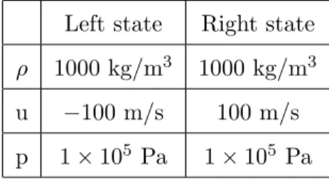
The simulation time is 0.2 ms, the discretization is of 1000 cells. The length of the computational domain is 1 m. The initial data are given in Table 2, and the numerical parameters for the stiffened gas law are given in Table 4.

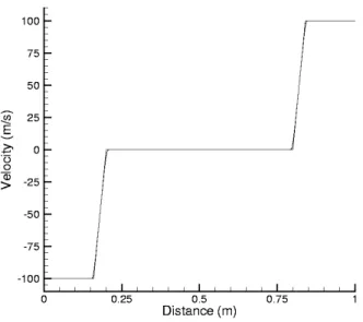
The numerical results are on Figures 2, 3, 4. We observe two rarefaction waves moving in opposite directions and the appearance of negative pressures in the rarefied region. Actually, negative pressures can locally and briefly appear in a liquid, they should then be called tensions. But in the zone of negative pressures the liquid would then be in a metastable state and would be subject to vaporization. It must be pointed out that if the cavitation is not taken into account, the appearance of negative pressures is neither a mathematical nor a numerical problem. For example, the model is still hyperbolic. For more details on this subject, we refer to our previous work [4].

We observe also a small undershoot on the density plot (Figure 2) in the center of the rarefaction. This undershoot is classical in the computation of rarefaction waves for single fluid flows with the Godunov scheme. Numerical tricks to avoid this phenomenon are detailed in [28].

Left state Right state ρ 1000 kg/m3 1000 kg/m3 u −100 m/s 100 m/s p 1 × 105 _{Pa 1 × 10}5 _Pa

Table 2

Initial data for the Riemann problem

Fig. 3. Comparison of the exact and numerical velocities in the metastable case

Fig. 4. Comparison of the exact and numerical pressures in the metastable case 5.2 Numerical results for the transition case

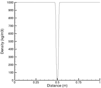
In this part, the second sub-step (optimization of the entropy) is activated. On the same test case as above, we obtained the results of Figures 5, 6, 7, 8, 9.

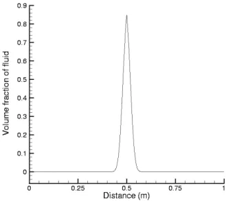
We observe that the pressure remains positive and that a vapor bubble ap-pears in the center of the computational domain, but this is only a qualitative

validation. We observe small perturbations of the pressure on Figure 7. These perturbations are localized in the cavitation region and decrease when the mesh is refined. Let us note that the test case is rather stiff: the pressure drops almost to zero. A slightly larger velocity in the initial conditions (ta-ble 2) would have implied a vacuum appearance in the vapor phase. Despite the stiffness of the case the calculation ended without complication and this indicates the robustness of the entropy maximization scheme.

Fig. 5. Density in the transition case

Fig. 7. Pressure in the transition case

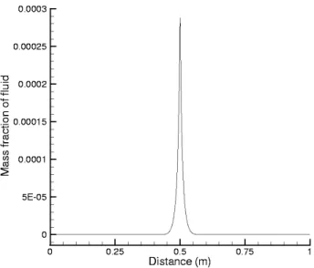
Fig. 8. Vapor volume fraction in the transition case 5.3 Comparison with the analytical solution

We also verify quantitatively that we are able to reproduce the physical en-tropy solution constructed in Section 4. It is important to notice here that the numerical solution does not depend on the CFL number. We explain the good behavior of the projection scheme by the fact that the production of entropy occurs not only in the Godunov step but also because of the phase transition. This is important because a global entropy production is not sufficient. One

Fig. 9. Vapor mass fraction in the transition case

could imagine, for example, a non-physical shock in the metastable model, with a local decrease of entropy, compensated by the entropy production due to the phase transition. The global entropy production can be positive, but the solution is not physical.

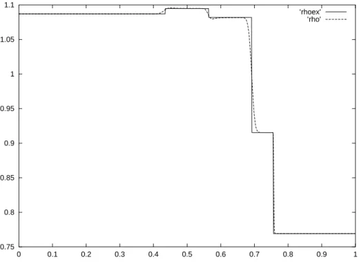
In this section, we present the numerical results obtained with the projection scheme for the analytical solution presented in Section 4.2. Numerical results are given in Figures 10, 11, 12. We observe an excellent agreement between the numerical and the exact solutions. The presented results have been ob-tained with a CFL number of exactly one and a number of 1000 cells. There is no oscillation and the viscous (or Liu’s) solution is well captured. We have also performed tests for lower CFL numbers and captured exactly the same solution. Other one-dimensional tests can be found in [3]. Let us recall that classical Godunov-type schemes can converge to various entropy solutions ac-cording to the CFL number as observed by Jaouen in [18].

6 The underwater projectile

This section is devoted to a 2D simulation in order to illustrate the ability of our scheme to deal with physical configurations. This test is very similar to the one proposed by Butler, Cocchi and Saurel in [28]. The goal is to compute the flow around a fast projectile diving into water at a velocity of 1000 m/s. A strong pressure loss appears in the wake of the projectile, triggering the growth of a cavitation pocket.

0.75 0.8 0.85 0.9 0.95 1 1.05 1.1 0 0.1 0.2 0.3 0.4 0.5 0.6 0.7 0.8 0.9 1 ’rhoex’ ’rho’

Fig. 10. Numerical and exact density for the relaxation scheme

-0.02 0 0.02 0.04 0.06 0.08 0.1 0.12 0.14 0 0.1 0.2 0.3 0.4 0.5 0.6 0.7 0.8 0.9 1 ’vitex’ ’vit’

Fig. 11. Numerical and exact velocity for the relaxation scheme 6.1 Tuning of the temperature law

We have first to compute adequate pressure law coefficients in order to obtain realistic results. In order to fix the constants, we have tried to respect some physical realities such as saturation curve, specific heat, sound speed.

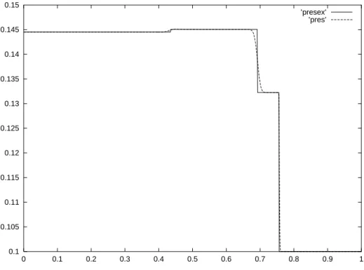
0.1 0.105 0.11 0.115 0.12 0.125 0.13 0.135 0.14 0.145 0.15 0 0.1 0.2 0.3 0.4 0.5 0.6 0.7 0.8 0.9 1 ’presex’ ’pres’

Fig. 12. Numerical and exact pressure for the relaxation scheme

At temperature T = 372.76K, the known physical values are reproduced in Table 3 and are extracted from the book of Lide [22].

Vapor Water

Enthalpy : h (J·g−1) 2674.9 × 103 417500

γ 1.3 3.

Cp (J·kg−1·K−1) 2100 4200

Table 3

Experimental values for the setting of the temperature law Thanks to the relation

h = Q + CpT, (73)

where h is the enthalpy, Q the energy of formation and Cp the specific heat at

constant pressure, we are able to compute the values of Q1 and Q2 :

Q1 = 0.1892 × 107J/kg, (74)

Q2 = −0.1148 × 107J/kg. (75)

The computation of the pressure constant π2 for the liquid water is based

1600 m.s−1 _{at ambient pressure and temperature. Then, thanks to the relation}

π2 =

ρ0c2

γ2

, (76)

where ρ0 = 1000 kg · m−3 is the density of water at ambient pressure and

temperature, we obtain π2 = 8533 × 105 Pa. In vapor π1 = 0 Pa.

In order to compute the constant K appearing in (52), we use the values of the specific heats at constant volume given in [22]:

Cv,1 = Cp,1 γ1 = 1615.38 J.kg−1.K−1 (77) Cv,2 = Cp,2 γ2 = 1400 J.kg−1.K−1 (78)

Finally, the constant K is obtained by

K = (Cv,1−Cv,2) ln(T0) + (79) (Q2−Q1) T0 + (γ1−1)Cv,1ln à (γ1−1)Cv,1T0 (p0+ π1) ! (80) −(γ2−1)Cv,2ln à (γ2 −1)Cv,2T0 (p0+ π2) ! ,

The ambient pressure is p0 = 105Pa and the ambient temperature T0 =

273.76K.

The physical constants of the stiffened gases model are summed up in Table 4.

fluid 1 (vapor) fluid 2 (water)

γ 1.3 3

π 0 8533 bar

Q 0.1892×107 _{J/kg -0.1148×10}7_J/kg

Cv 1615.38 J/kg/K 1400 J/kg/K

Table 4

Constants in the stiffened gas model

6.2 Numerical results

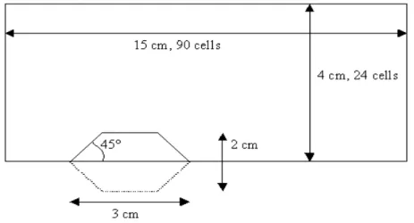
In this part, we present the numerical results in 2D. The projectile and the computational domain are described in the graphic 13. The horizontal velocity

of the projectile is −1000 m.s−1_{, it is thus moving from the right to the left. By}

a change of reference frame, we can also suppose that the projectile is fixed and impose a velocity of water of 1000 m.s−1_{. On the boundary of the projectile,}

Fig. 13. Geometry description

the upper and the lower parts of the domain boundary, we impose a mirror condition. On the inner and outer parts of the boundary, we impose the nature of the flow: ρ = 1000 kg.m−3, p = 105 _{Pa, horizontal velocity u = 1000 m.s}−1_,

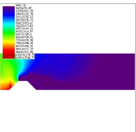
vertical velocity v = 0. We take the same values for the initial condition in the domain in order to model the sudden arrival of the projectile in the water. The pressure and the volume fraction of water are represented at time t = 225 µs on Figures 14 and 15.

7 Conclusion

In this paper, we have first constructed a model for liquid-vapor phase transi-tion. Returning to thermodynamics we have shown how to properly construct pressure laws for a mixture of two fluids. It appears that the equilibrium pres-sure law corresponds to a maximum of the mixture entropy with respect to the volume, mass and energy fractions of the vapor. Using this representation, it was possible to propose a new projection finite volume scheme for the nu-merical simulation of cavitation. Each time step of this scheme is made up of two stages. In a first stage, the flow is solved by a classical Godunov scheme with exact Riemann solver, without taking into account phase transition. This is possible because the mixture pressure law is simpler than the equilibrium pressure law. In a second stage, the fractions are updated in order to recover the equilibrium pressure law by a maximization of the mixture entropy. This scheme was first tested on an analytical solution. It was able to recover the unique physical solution, the Liu solution, even if several entropy solutions are

Fig. 14. Pressure (Pa) at 225 µs

possible. Finally, we illustrated the ability of the scheme to deal with more physical configurations in 2D.

This work could be extended in several directions:

(1) First of all, it would be interesting to improve the precision of the mixture law. Indeed, in its present form, the model is only valid below the critical point. The critical point is a special point of the phase diagram in the temperature-pressure plane. It corresponds to the upper extremity of the saturation curve. Beyond this point there is no more distinction between the two phases. We hope that this behavior can be modelled, at least roughly, by only changing the entropy function of the liquid phase. (2) Another interesting extension would be to add a supplementary inert

phase in order to simulate, for instance, air-water flows, with the possi-bility to observe a cavitation phenomenon in water. The model is a simple extension of what is done in Section 2.3. The mixture entropy is the sum of the three phases entropies, as in formula (29), and depends on density, internal energy, air fractions and vapor fractions. In the optimization pro-cess, we maximize the mixture entropy with respect to all the fractions excluding the mass fraction of air, because there is no mass transfer be-tween air and water. The mass fraction of air is thus simply convected.

Fig. 15. Vapor volume fraction at 225 µs

Despite its simplicity this approach leads to numerical difficulties. Ac-cording to our first experiments, numerical pressure oscillations appear at the interface between air and water [3]. These oscillations are similar to those observed in many works about two-phase flows [1], [19], [27], [31]... It must be pointed out that in the present work we observed no pressure oscillations at the interface between liquid and vapor for we have allowed mass transfers between these two phases. The maximization of entropy ensures the good stability of the numerical scheme. On the other hand, if the optimization with respect to one variable is omitted (it would be the case for an interface without mass transfer), it is sufficient to imply oscillations.

(3) Finally, it appears that the equilibrium hypothesis is physically not true for very fast flows. It is even possible to observe during a short time negative pressures in the liquid before the phase transition [12]. It is clear that one should then give a finite value to the parameter λ in the source term (17). This value is linked to the time scale of the phase transition. Instead of solving numerically an ordinary differential equation one could imagine for instance to perform only a partial optimization of the mixture entropy.

References

[1] R. Abgrall. Generalisation of the Roe scheme for the computation of mixture of perfect gases. Recherche A´erospatiale, 6:31–43, 1988.

[2] S. Andreae, J. Ballmann, S. M¨uller, and A. Voss. Dynamics of collapsing bubbles near walls. In Ninth International Conference on Hyperbolic Problems. IGPM, RWTH, Aachen, 2002.

[3] T. Barberon. Mod´elisation math´ematique et num´erique de la cavitation dans les ´ecoulements multiphasiques compressibles. PhD thesis, Universit´e de Toulon, December 2002.

[4] T. Barberon, P. Helluy, and S. Rouy. Practical computation of axisymmetrical multifluid flows. International Journal of Finite Volumes, 1(1):1–34, 2003. [5] H. Bethe. The theory of shock waves for an arbitrary equation of state. Technical

report, US department of commerce, 1942.

[6] H. B. Callen. Thermodynamics and an introduction to thermostatistics, second edition. Wiley and Sons, 1985.

[7] G. Chanteperdrix, P. Villedieu, and Vila J.-P. A compressible model for separated two-phase flows computations. In ASME Fluids Engineering Division Summer Meeting. ASME, Montreal, Canada, July 2002.

[8] J.-P. Cocchi and R. Saurel. A Riemann problem based method for the resolution of compressible multimaterial flows. Journal of Computational Physics, 137(2):265–298, 1997.

[9] F. Coquel and B. Perthame. Relaxation of energy and approximate Riemann solvers for general pressure laws in fluid dynamics. SIAM J. Numer. Anal., 35(6):2223–2249 (electronic), 1998.

[10] J.-P. Croisille. Contribution `a l’´etude th´eorique et `a l’approximation par ´el´ements finis du syst`eme hyperbolique de la dynamique des gaz multidimensionnelle et multiesp`eces. PhD thesis, Universit´e Paris VI, 1991. [11] S. Dellacherie. Relaxation schemes for the multicomponent Euler system. M2AN

Math. Model. Numer. Anal., 37(6):909–936, 2003.

[12] J.-P. Franc et al. La Cavitation: M´ecanismes Physiques et Aspects Industriels. Presses Universitaires de Grenoble, 1995.

[13] T. Gallou¨et, J.-M. H´erard, and N. Seguin. Some recent finite volume schemes to compute Euler equations using real gas EOS. Internat. J. Numer. Methods Fluids, 39(12):1073–1138, 2002.

[14] E. Godlewski and P.-A. Raviart. Numerical approximation of hyperbolic systems of conservation laws. Springer, 1996.

[15] B. T. Hayes and P. G. Lefloch. Nonclassical shocks and kinetic relations: strictly hyperbolic systems. SIAM J. Math. Anal., 31(5):941–991 (electronic), 2000.

[16] P. Helluy. M´emoire d’habilitation `a diriger des recherches: Quelques exemples de m´ethodes num´eriques r´ecentes pour le calcul des ´ecoulements multiphasiques. http://helluy.univ-tln.fr/ADMIN/habilitation.pdf. (french), 2004. [17] P. Helluy and T. Barberon. Finite volume simulations of cavitating flows. In

Finite Volumes for Complex Applications III (Porquerolles, 2002), pages 455– 462. Hermes Penton Ltd, London, 2002.

[18] S. Jaouen. Etude math´ematique et num´erique de stabilit´e pour des mod`eles´ hydrodynamiques avec transition de phase. PhD thesis, Universit´e Paris VI, November 2001.

[19] S. Karni. Multicomponent flow calculations by a consistent primitive algorithm. J. Comput. Phys., 112(1):31–43, 1994.

[20] B. Koren, M. R. Lewis, E. H. van Brummelen, and B. van Leer. Riemann-problem and level-set approaches for homentropic two-fluid flow computations. J. Comput. Phys., 181(2):654–674, 2002.

[21] P. G. LeFloch and C. Rohde. High-order schemes, entropy inequalities, and nonclassical shocks. SIAM J. Numer. Anal., 37(6):2023–2060, 2000.

[22] D. R. Lide et al. Handbook of chemistry and physics, 82nd

edition. CRC Press, 2001.

[23] T. P. Liu. The Riemann problem for general systems of conservation laws. J. Diff. Equations., 56:218–234, 1975.

[24] R. Menikoff and B. J. Plohr. The Riemann problem for fluid flow of real materials. Rev. Modern Phys., 61(1):75–130, 1989.

[25] B. Perthame. Boltzmann type schemes for gas dynamics and the entropy property. SIAM J. Numer. Anal., 27(6):1405–1421, 1990.

[26] R. Saurel and R. Abgrall. A multiphase Godunov method for compressible multifluid and multiphase flows. J. Comput. Phys., 150(2):425–467, 1999. [27] R. Saurel and R. Abgrall. A simple method for compressible multifluid flows.

SIAM J. Sci. Comput., 21(3):1115–1145, 1999.

[28] R. Saurel, J.P. Cocchi, and P.B. Butler. A numerical study of cavitation in the wake of a hypervelocity underwater projectile. AIAA Journal of Propulsion and Power, 15(4):513–522, 1999.

[29] D. Serre. Syst`emes de lois de conservation I et II. Diderot Editeur, 1996. [30] E. F. Toro. Riemann solvers and numerical methods for fluid dynamics, 2nd

edition. Springer, 1999.

[31] E. H. van Brummelen and B. Koren. A pressure-invariant conservative Godunov-type method for barotropic two-fluid flows. Journal of Computational Physics, 185:289–308, 2003.

[32] B. Wendroff. The Riemann problem for materials with non-convex equations of state: II, general flows. J. Math. Anal. Appl., 38:640–658, 1972.

[33] H. Weyl. Shock waves in arbitrary fluids. Com. Pure Appl. Math., 103(2):103– 122, 1949.