Biomolecular System Design: Architecture, Synthesis, and Simulation

(1)

HAL Id: tel-01237638

https://hal.inria.fr/tel-01237638

Submitted on 3 Dec 2015

HAL is a multi-disciplinary open access

archive for the deposit and dissemination of sci-entific research documents, whether they are pub-lished or not. The documents may come from teaching and research institutions in France or abroad, or from public or private research centers.

L’archive ouverte pluridisciplinaire HAL, est destinée au dépôt et à la diffusion de documents scientifiques de niveau recherche, publiés ou non, émanant des établissements d’enseignement et de recherche français ou étrangers, des laboratoires publics ou privés.

Katherine Chiang

To cite this version:

Katherine Chiang. Biomolecular System Design: Architecture, Synthesis, and Simulation. Program-ming Languages [cs.PL]. National Taiwan University, 2015. English. �tel-01237638�

(2)

國立臺灣大學電機資訊學院電子工程學研究所

博士論文

Department or Graduate Institute of Electronics Engineering

College of Electrical Engineering and Computer Science

National Taiwan University

Doctoral Dissertation

生物分子計算系統設計：架構、合成、與模擬

Biomolecular System Design:

Architecture, Synthesis, and Simulation

姜慧如

Katherine H. Chiang

指導教授

(Advisors):

江介宏

博士 (Jie-Hong R. Jiang, Ph.D.)

François Fages, Ph.D.

中華民國

104 年 6 月

June 2015

國立臺灣大學電子工程學研究所博士論文

生

物

分

子

計

算

系

統

設

計

：

架

構

、

合

成

、

與

模

擬

姜

慧

如

撰

6

(3)

Architecture, Synthesis, and Simulation

By

Katherine H. Chiang

Advisors: Dr. Jie-Hong R. Jiang and Dr. François Fages

Graduate Institute of Electronics Engineering

National Taiwan University

Abstract

The advancements in systems and synthetic biology have been broadening the

range of realizable systems with increasing complexity both in vitro and in vivo.

Systems for digital logic operations, signal processing, analog computation, program

flow control, as well as those composed of different functions – for example an

on-site diagnostic system based on multiple biomarker measurements and signal

processing – have been realized successfully. However, the efforts to date tend to

tackle each design problem separately, relying on ad hoc strategies rather than

providing more general solutions based on a unified and extensible architecture,

resulting in long development cycle and rigid systems that require redesign even for

small specification changes.

Inspired by well-tested techniques adopted in electronics design automation

(EDA), this work aims to remedy current design methodology by establishing a

standardized, complete flow for realizing biomolecular systems. Given a behavior

specification, the flow streamlines all the steps from modeling, synthesis, simulation,

to final technology mapping onto implementing chassis. The resulted biomolecular

systems of our design flow are all built on top of an FPGA-like reconfigurable

architecture with recurring modules. Each module is designed the function of each

(4)

module depends on the concentrations of assigned auxiliary species acting as the

“tuning knobs.” Reconfigurability not only simplifies redesign for altered

specification or post-simulation correction, but also makes post-manufacture

fine-tuning – even after system deployment – possible. This flexibility is especially

important in synthetic biology due to the unavoidable variations in both the deployed

biological environment and the biomolecular reactions forming the designed system.

In fact, by combining the system’s reconfigurability and neural network’s

self-adaptiveness through learning, we further demonstrate the high compatibility of

neuromorphic computation to our proposed architecture. Simulation results verified

that with each module implementing a neuron of selected model (ex. spike-based,

threshold-gate-like, etc.), accompanied by an appropriate choice of reconfigurable

properties (ex. threshold value, synaptic weight, etc.), the system built from our

proposed flow can indeed perform desired neuromorphic functions.

(5)

1 Introduction 1

1.1 Motivation . . . 1

1.2 Our contributions . . . 2

1.3 Structure of the thesis . . . 4

2 Hybrid simulation of heterogeneous reaction models 7 2.1 SBML reaction rules and events . . . 12

2.1.1 Reaction rules and kinetics . . . 12

2.1.2 Events . . . 14

2.2 Hybrid continuous-stochastic models . . . 17

2.2.1 Gillespie’s stochastic simulation algorithm (SSA) . . . 18

2.2.2 Event-based implementation of SSA . . . 19

2.2.3 Preprocessor for composing continuous and stochastic models 21 2.3 Dynamic strategies for hybrid continuous-stochastic simulations . . . 24

2.3.1 Dynamic partitioning criteria . . . 25

2.3.2 Implementation . . . 26

2.3.3 Simple example . . . 28

2.3.4 Performance evaluation . . . 30

2.4 Hybrid Boolean models . . . 35 2.4.1 Preprocessor for composing continuous and Boolean models . 35

(6)

Contents

2.4.2 Hybrid composition of continuous-Boolean models . . . 37

2.4.3 Stochastic-continuous-Boolean model simulation . . . 40

3 Reconfigurable biochemical reaction systems synthesis 41 3.1 Modeling language . . . 41

3.2 Reconfigurable logic cicuit synthesis . . . 42

3.2.1 Configurable logic units . . . 44

3.2.2 Configurable interconnects . . . 48

3.2.3 Retroactivity resistance . . . 49

3.2.4 Multiplexer-based structure . . . 51

3.2.5 Case study . . . 54

3.3 Level-based neuromorphic computation . . . 58

3.3.1 Artificial neural network and adopted neuron model . . . 61

3.3.2 General architecture of neuromorphic FPGA . . . 63

3.3.3 Neuron module . . . 66

3.3.4 Programmable interconnect . . . 70

3.3.5 Resource requirement . . . 71

3.3.6 Case study: classifier synthesis with known criteria . . . 71

3.3.7 Case study: classifier synthesis with learning ability . . . 75

3.4 Spike-based neuromorphic computation . . . 77

3.4.1 Adopted neuron model and key properties . . . 79

3.4.2 Directional signal transmission with waveform preserved . . . 81

3.4.3 Neuron module . . . 82

4 Technology mapping and implementation 85 4.1 Enzyme . . . 86

(7)

4.1.2 Reaction motifs . . . 94

4.1.3 Mapping example: configurable Boolean logic gate . . . 95

4.2 DNA strand displacement . . . 100

4.2.1 DSD reaction modules as mapping target . . . 103

4.2.2 Reaction rate . . . 103

4.2.3 Mapping example: circuit . . . 103

4.2.4 Mapping example: classifier . . . 104

5 Conclusions and future work 112 A DSD simulation code 113 A.1 Code for mapping example: circuit . . . 113

A.2 Code for mapping example: classifier . . . 117

B Hudgkin-Huxley model simulation 122 B.1 Code for mapping example: circuit . . . 122

List of Figures 129

List of Tables 131

(8)

Chapter 1 Introduction

1.1 Motivation

The advancements of synthetic biology have been broadening the range of realizable systems of increasing complexity both in vivo and in vitro. Building systems within a biochemical world is not far from reach and has been intensively studied, e.g., in terms of digital logic operations [37, 47, 63], analog computation [20], linear control [17, 60], signal processing [48], program flow control [44], etc. The bio-compatibility of such systems is unique in that they can not only allow effective interfacing between physiological processes and nano-structured materials as well as electronic systems, but can further embed computation tasks that integrate sensing, information processing, and actuation, inside living cells without physical intrusion. However, most, if not all, of existing engineered biochemical systems perform specific functions with fixed parametric values, which once designed, cannot be changed. This static approach toward functions and parameters is preferred for

(9)

design analysis and verification, but can be seriously disadvantageous when the uncertainty involved in environmental evolution is influential to the systems’ behavior, or when the systems’ behavior cannot be fully determined in the design phase. Even for electronic system design—which is relatively very predictable as hinted by the existence of clearly defined datasheets—it is still not uncommon that a design has to be rectified after it is manufactured. Likewise in biochemical system design, reconfigurability is beneficial and usually crucial because of the intrinsically stochastic biochemical environments. While the reconfigurability of integrated circuits (ICs) can be achieved through embedding firmware or programmable gate arrays into the design, it remains unclear how a similar mechanism can be economically embedded into a biochemical design.

Inspired by the success achieved by electronics design automation (EDA) method-ology in efficiently realizing systems of fast-growing complexity, flexibility, and robustness, we tried to address this deficiency by proposing a new synthetic biology design framework with lessons learned from EDA to deal with shared concerns, while also modified to take into account the fundamental differences of the two engineering paradigms.

1.2 Our contributions

The proposed framework is based on a flexible, modular architecture that is similar to a field programmable gate array (FPGA). Specifically, emphasis is placed on the resulted systems’ reconfigurability, which is of crucial importance for system reliability in the biochemical world, where variations of common degree can cause serious functional deviations in the deployed systems. In this work, the choice of

(10)

1.2. Our contributions

adopting chemical reaction network (CRN) as the middle description language for bridging the user specifications to kinetics desired of molecular interactions is not only based on the fact proved in [72] that CRNs form a Turing-universal computational model capable of encoding any kind of computational behavior, but also on its being standardized and well-accepted across various disciplines.

In the proposed design framework, a flow for realizing biomolecular systems as well as its accompanying reservoirs of standardized modules (motifs) are constructed. Given a behavior specification, the proposed framework synthesizes the specification to a CRN that is amenable to final implementations using enzyme reactions and/or DNA strand displacement. The flow streamlines all steps from processing system behavior specification until right before where the wetlab experiments would join in the future— from modeling, synthesis, simulation, to final technology mapping onto implementing chassis of choice. The accompanying reservoirs of reconfigurable modules are designed with loading effects (retroactivities) considered. Different reservoirs of modules are prepared not only for different classes of specialized func-tionalities (ex. Boolean logic operations or neuromorphic computations), but also for different technology mapping targets—we try to have the structure of chemical reaction network (CRN) in the modules more similar to that of the existing ones presented in targeted chassis—in order to increase the probability that the modules can be more directly mapped to existing reactions.

Apart from taking care of the above considerations, two other novel extensions are made to the framework:

First, multiple kinds of system specification are allowed to accommodate the richness and uncertainty of biochemical applications. Current available options include:

(11)

• neuromorphic algorithm with interconnects and update functions specified; • training datasets based on which the system would learn the unknown “correct”

function, and would automatically evolve to realize the function learned.

Second, this work takes an important step toward embedding the power of neural networks into a broader range of biological systems. A correspondence between the information transmission mechanisms of ubiquitous cell signaling pathways and the action potential propagation in neurons of Hodgkin-Huxley model is established. Based on the correspondence, we propose an analog approach to realize reconfigurable neuromorphic computation using existing biochemical reactions of signaling pathways for better bio-compatibility.

1.3 Structure of the thesis

This thesis is organized as follows:

• Chapter 2 shows a new, nonstandard way to define stochastic and Boolean simulators by properly combining reaction rules and events, justifying the hy-brid composition and simulation of heterogeneous biochemical reaction models. Specifically, a high-level interface is implemented to show how two SBML models of different interpretations can be effectively composed into one. Furthermore, dynamic partitioning strategies for automatically partitioning reactions into stochastic or continuous interpretations based on adaptive criteria are pre-sented, with gain in both accuracy and simulation time compared to static partitioning.

(12)

1.3. Structure of the thesis

events, which will serve as the two components for our heterogeneous model construction, and whose kinetics will be used to capture, or approximate, that of the modeled system for hybrid simulation.

Section 2.2 presents the non-standard way of using event to embed stochastic reaction occurrences into continuous system evolution. A proof-of-concept implementation of a preprocessor that can automatically generate reaction-event-based hybrid models is presented in the end.

In Section 2.3, considering the fact that all interpretations have their respec-tive applicable conditions, strategies for dynamically adjusting the interpreta-tions of the reacinterpreta-tions during system evolution are presented and implemented to more accurately capture the behavior under live condition.

Section 2.4 focuses on hybrid model construction with Boolean semantics involved. Boolean semantics provides an effective way to capture switch-like behavior as that demonstrated in genetic networks, and a natural interface with finite state machine.

• Chapter 3 is devoted to the biochemical reaction synthesis of our proposed reconfigurable architectures. Different specification formats are provided so that system requirements can be specified in formats that can accurately portrait the desired behaviors in a convenient way. Firstly in Section 3.1, the motivation of our choice of using chemical reaction network (CRN) as the description language is given. CRN forms the bridge between behavior specification to required kinetics in the sense that once fulfilled, the desired behavior can be realized.

The synthesis of reconfigurable logic specification is presented in Section 3.2. The system is based on reconfiguable logic gates whose functions can be switched between a set of functional complete logic operations simply by

(13)

concentration controls. The architecture is very similar to the FPGA, except that the species used for different gates should not introduce “undesigned” interactions.

In Section 3.3 and Section 3.4, the synthesis of neuromorphic computation based on threshold gate-like binary neuron model and spike-timing based neu-ron model are presented respectively.

• The networks of reactions synthesized as described in Chapter 3 all have CRN-modeled behavior that, theoretically, satisfy the specified requirements. Chapter 4 shows the preliminary attempt to map the synthesized designs to realistic biochemical reactions based on real-world motifs extracted from existing reactions of targeted chassis.

The mapping to two kinds of targeted chassis are discussed. In Section 4.1, the enzyme realization of kinetics described by CRNs is presented along with the kinetics motifs based on six standard types of enzyme-catalyzed reactions. In Section 4.2, we go through the well-established mapping relations between CRN and DNA strand displacement kinetics, and used Visual DSD simulation of the accordingly mapped strands as the verification of our proposed synthesis method.

• Finally, Chapter 5 concludes this work and outlines possible directions for future work.

(14)

Chapter 2 Hybrid simulation of

heterogeneous reaction models

Systems biology aims to elucidate the high-level functions of the cell from their biochemical basis at the molecular level [46]. A lot of work has been done for collecting genomic and post-genomic data, making them available in databases [6,49], and organizing the knowledge on pathways and interaction networks into models of cell metabolism, signaling, cell cycle, apoptosis, etc., many of which are published in model repositories such as http://biomodels.net/. Aiding the efforts, the Systems Biology Markup Language (SBML) [45] provides a common exchange format for biochemical reaction systems and is nowadays supported by a majority of modeling tools.

According to the knowledge available on the system and to the nature of queries expected to be answered by the model, e.g. qualitative or quantitative predictions, these rule-based reaction systems can be interpreted (and simulated) under different semantics as either:

(15)

• ordinary differential equations (continuous semantics), • continuous-time Markov chains (stochastic semantics), • Petri nets (discrete semantics),

• Boolean transition systems (Boolean semantics), and many variants.

These different interpretations can be related by either approximation [30–32] or abstraction [23] relationships. Many modeling tools support several of them but provide no support for the combination of heterogeneous models. However, in the perspective of applying engineering methods to the analysis and control of biological systems, the issue of building complex models by composition of elementary models is a central one. While reaction systems can be formally composed by the multiset union of reaction rules, and interpreted by one common semantics, there is also a need to compose models with different semantics preserved, as will be clearly shown in this section by some examples from the literature. What we call a hybrid model is a model obtained by composing models of heterogeneous semantics (continuous, stochastic, Boolean, etc.), and hybrid simulation is the topic of simulating such hybrid models.

In [61], the author observes that “A very promising direction is the development of hybrid methods because they directly deal with the important problem of stiffness, which is often present in biochemical models. [. . . ] There exist already a few software tools, which allow for hybrid simulation, [. . . ] and this number is expected to grow in the future.” In this chapter, we propose a general approach to progress in that direction by showing that the combination of reaction rules and events, as already present in SBML, can be used in a non-standard way to give meaning to the hybrid composition and simulation of heterogeneous reaction models. In particular, we show

(16)

Chapter 2. Hybrid simulation of heterogeneous reaction models

how hybrid continuous-Boolean models and hybrid continuous-stochastic models can be assembled and simulated, through the specification of a high-level interface for composing heterogeneous models, and producing as output a hybrid model in standard SBML format, which can thus be executed with any SBML-compatible simulator.

Our high-level interface, prototyped in the modeling environment Biocham [13, 24], takes two models with synchronization information as inputs, and produces one SBML model with reactions and events as output. For hybrid continuous-Boolean composition, it transforms a Boolean state transition model to events with extra triggers which express the links with the continuous variables and the parameters of the continuous reaction model. For hybrid continuous-stochastic composition, the interface described in this chapter transforms stochastic reactions to a set of events, which implements Gillespie’s direct method for stochastic simulation, and can be freely combined with the simulation of continuous reactions. Furthermore, our framework supports the specification of dynamic strategies which automatically choose between the stochastic and continuous interpretations of the reactions according to particle counts, reaction propensities, or more specific model-dependent criteria. We show that without the need to conduct time-consuming fully stochastic simulations beforehand to obtain the scale information of particle count and propensity for all reactions, dynamic partitioning results in higher accuracy and shorter simulation time than static partitioning – as static partitioning cannot adapt to the possibly substantial scale variations over time, which can render the initial partition inadequate.

This approach is illustrated and evaluated with several examples including the reconstructions of the hybrid model of the mammalian cell cycle regulation of Singhania et al. [71] as the composition of a Boolean model of cell cycle phase

(17)

transitions and a continuous model of cyclin activation, plus a hybrid Boolean-continuous-stochastic version of this model with dynamic partitioning strategy, and of the hybrid stochastic-continuous model of bacteriophage T7 infection of Alfonsi et al. [4], and of bacteriophage λ of Goutsias [40], showing the gain in both accuracy and simulation time of the dynamic strategy.

Since XML, and hence SBML, are not easy to read by humans, in this thesis, we use mathematical notation and Biocham code for clarity purpose. The Biocham and SBML files of the examples of this chapter are available at: http://lifeware. inria.fr/supplementary_material/TOMACS/. The Biocham files can be executed via the Biocham web application http://lifeware.inria.fr/biocham/online without any installation.

Related work

Hybrid simulation is a classical topic in physics, e.g. for numerically solving equations describing stochastic systems using ordinary differential equations whenever possible in place of stochastic equations, in order to speed-up simulations [4, 67]. It is also ubiquitous in computer science for programming and verifying hybrid systems which have both discrete and continuous dynamics [5, 39]. Hybrid modeling is also used in Systems Biology for reducing the complexity of many modeling task, e.g. [1, 5, 9, 11, 27, 51, 58, 71], for speeding up stochastic simulations [33, 36, 40, 68], and achieving whole cell simulation [50]. A review of the different approximate stochastic and hybrid methods used in Systems Biology can be found in [61].

Due to the structure of SBML, which mostly relies on explicit and global reactions and events, the composable modelling at the core of hybrid process algebra, e.g. [3,26]

(18)

Chapter 2. Hybrid simulation of heterogeneous reaction models

is out of reach of the presented work. On the other hand, we show that SBML can express various form of hybrid systems. Indeed, a set of SBML events and continuous reactions can also be visualized as a hybrid automaton [38] in which there is a state with a particular ODE for each combination of the trigger values, and there is a transition from one state to another state when at least one trigger changes value from false to true in the source state. Stochastic hybrid automata [34] can be similarly simulated in SBML with a random number generator coded by events. Since our focus in this chapter is on SBML, we are mainly focused on simulations and on the reproduction of simulation results, as examplified for instance by the notion of “curated” model in the BioModels project at http://biomodels.net/. The use of existing verification tools for hybrid systems is thus beyond the scope of this thesis.

Another line of work also exists on the extension of Boolean models with con-tinuous time delays. Ren´e Thomas’s discrete modeling of gene regulatory networks (GRN) [73] is a well known approach to study the logical dynamics of a set of interacting genes. It deals with a graph of positive and negative influences between genes and logical functions that determine the possible trajectories in the state space. Those parameters are a priori unknown, but they may generally be deduced from a large set of biologically observed behaviors in various conditions. Besides, it neglects the time delays for a gene to pass from one level of expression to another one. In [1], it is shown that one can account for time delays depending on the expression levels of genes in a GRN, while preserving powerful enough computer-aided reasoning capabilities. The characteristic of this approach is that, among possible execution trajectories in the model, one can automatically find out both viability cycles and ab-sorption in capture basins. Model-checking techniques developed for hybrid systems are used for this purpose [2]. The authors describe a Hybrid model for the mucus

(19)

production in the bacterium Pseudomonas aeruginosa and show that they are able to discriminate between various possible dynamical behavior [1, 2]. Such a model can be presented and compiled in a set of reaction rules with events as described in this thesis.

Time constraints provide another means to refine Boolean or discrete models which are often too coarse to be useful. In [56], the authors present a new technique for over-approximating (in the sense of timed trace inclusion) continuous dynamical systems by timed automata for the purpose of efficiently checking timed (as well as untimed) properties. The essence of this technique is the partition of the state space into cubes and the allocation of a clock for each dimension. This is in contrast with other approaches which use only one clock. This idea is a specific case of rectangular hybrid automata. This makes it possible to get better approximations of the behavior. The timed automata produced by these techniques can be similarly composed in our tool for simulation.

2.1 SBML reaction rules and events

2.1.1 Reaction rules and kinetics

In SBML [45], a reaction rule is composed of a reaction rate, a left- and a right-hand side of molecular species, with corresponding stoichiometric coefficients. In this thesis, an SBML reaction i written in mathematical notation:

X

j

lij× Sj vi

(20)

2.1. SBML reaction rules and events

corresponds to the following code in Biocham syntax:

vi for X j lij∗Sj=> X rij∗Sj

where vi is any mathematical function (given in a subset of MathML notation in

SBML, and in Biocham with the abbreviation MA for mass action law kinetics) of the species concentrations and parameters of the system, which defines the rate of reaction i. A reaction model is a finite set of reactions.

Depending on the data available of the system and the nature of queries that the model aims to address to, e.g. qualitative or quantitative predictions, a reaction model can be interpreted under different semantics: continuous, stochastic, discrete or boolean.

The stochastic semantics, which would be detailed in Section 2.2.1, associates to a reaction model a Continuous-Time Markov Chain (CTMC), with states defined by molecular counts, transitions by reactions, and reaction rates equal propensities representing transition probabilities after normalization. The associated CTMC realizes the solution to the Chemical Master Equation [30] of the reaction model.

The continuous semantics associates to a reaction model an Ordinary Differential Equation (ODE) system of the following form:

d[Sj]

dt = X

i

(rij− lij)× vi

The ODE system describes the evolution of molecular species concentrations with time according to the reaction rates. The continuous semantics approximates the mean behavior of the CTMC for large numbers of molecules. The continuous semantics usually leads to numerical integration, whereas the stochastic semantics is either

(21)

used for exact or approximate simulation, or for stochastic model checking (see for instance [52]).

The discrete semantics of a reaction model can be formalized using a Petri net [28], which keeps the stoichiometric information but leaves out the reaction rates vi. The

Petri net semantics can be seen as an abstraction of the stochastic semantics. The Boolean semantics omits precise stoichiometry and keeps only information about whether or not a species is active. It can be defined as an abstraction of the previous discrete semantics, provided that the combinatorics of all possible consumptions is maintained [23]. The Boolean semantics of large networks is especially useful for efficiently proving reachability properties by symbolic model checkers [14] instead of directly performing simulations.

2.1.2 Events

SBML models also allow behavior description using events. An SBML event is basically composed of two parts: a trigger that specifies the condition for it to fire, and an action that describes its influence on current state (defined by concentrations and parameter values) in the form of a list of assignments. In this thesis, we will write an event in Biocham syntax as follows:

event(trigger, [s1, . . . , sn], [f1, . . . , fn])

where si’s indicate the variables that are modified by the event, and fi’s the

mathe-matical functions of the state variables that give the new value to si’s.

(22)

2.1. SBML reaction rules and events

concept is the same: that an event fires when its triggering condition changes from false to true. This induces however several issues:

• what happens at the start of the simulation?

• how to determine the precise timing when a trigger condition turns to true? • what happens if more than one events are enabled simultaneously?

The first point is easy to settle. Whether events that are true at time 0 should fire or not is an arbitrary choice with no impacts on the expressive power of the formalism, since the influence of both choices can be absorbed into the setting of initial state. In the Biocham simulator used in this thesis, the choice is to avoid the firing of events at the initial point of the simulation; an event only gets triggered when its condition turns from false to true, i.e., it is the transition that matters. If an event is really meant to be triggered at the very beginning, the initial state is modified accordingly to reflect the changes in state variables caused by one firing of the event.

The second point, in fact, has been solved in practical tools for a long time: since numerical integration of ODEs goes by steps, one detects changes in triggers only in the interval of a simulation step. If some triggers become true, one can thus go back in time until one finds—with a given precision—the first time point where the first trigger becomes true. Note however that if arbitrarily complex conditions appear in the events, a numerical integrator unaware of the events can hide inside a single step that a trigger went from false to true and back to false again. Therefore, a cautious implementation is necessary, and fixed step size integration methods may be recommended to use in presence of events, instead of more efficient adaptive step size methods.

(23)

set of events that are enabled simultaneously at a given time will all be fired, whatever the actions of the events are, but what if several events modify the same variable? It is possible to assume a synchronous semantics, where the simultaneous events execute their actions in parallel, but then one must forbid events with conflicting actions, i.e., events that would modify in different ways the same variable at the same time point. A more common choice is an asynchronous semantics, that will fire all the events enabled at a given time one after the other. Conflicts in actions are then solved by the ordering of events, which can be either random, i.e. non-deterministic, or given by the user, e.g. by the order of writing (Biocham choice) or by priorities (SBML choice). However, if some actions invalidate the triggering condition of originally enabled events, these events should be disabled in a purely asynchronous semantics. The SBML Level 3 choice1 _{is to keep a very flexible semantics, with}

semi-asynchronous events, which can use either the values at the time they were enabled, or the current values at the time they are actually executed, after the execution of the simultaneous events with higher priority, and which can specify the permanence of an event in order to define if it should be fired even if its trigger has been invalidated by previous events firing at the same time.

In Biocham, there are no priorities, and the events that are enabled simultane-ously are executed in the order of their writing using current values. An event with n assignments of fi to si is therefore equivalent to the sequence of n events with

the same trigger for each assignment fi to si. The semantics of events implemented

in Biocham can thus be defined in SBML Level 3 using the current value and permanence options and priorities corresponding to the order of writing.

1_{The Versions and Releases of the SBML Level 3 Core specification and officially-supported}

Level 3 package specifications are available at: http://sbml.org/Documents/Specifications/ SBML_Level_3.

(24)

2.2. Hybrid continuous-stochastic models

It is worth noting that in SBML Level 3, thanks to the Distributions package, random variables can be represented. This would be useful in the following sections to implement stochastic semantics with SBML events. However, since the SBML Test Suite Database and the page of the Distributions package show that there is apparently no software currently able to cope both with prioritized events and random variables, we have implemented a simple linear pseudo-random number generator (PRNG) using SBML events. The files generated by our hybridization interfaces can therefore be run with any SBML Level 3 core compatible simulator.

2.2 Hybrid continuous-stochastic models

Chemical reactions, originated from random collisions of particles, are discrete and stochastic in nature. Although there is no way to predict the exact state of a chemical system at a specific time point, its statistical behavior can be effectively calculated from known probabilistic properties, as done by Gillespie’s stochastic simulation algorithm (SSA) [29], to be detailed in Section 2.2.1. The SSA simulation can be especially slow if one or more of the reactions have fast reaction rates (or high event occurrences) because the next reaction time will be very short due to the high probability of firing (one of the) fast reactions.

Despite the fact that all reactions are innately stochastic, those with large reactant counts and high reaction rates can be accurately approximated in terms of deterministic behavior expressed by ODEs. By incorporating both continuous and stochastic semantics into one simulator, an optimal balance between simulation runtime and accuracy can be achieved. This potentially lifts the scalability of simulating large biological systems. In Section 2.2.2, we provide an event-based view

(25)

on the SSA, that serves as basis to a hybrid continuous-stochastic simulator built upon an ODE simulator with events.

2.2.1 Gillespie’s stochastic simulation algorithm (SSA)

A reaction model with kinetic expressions can be interpreted under the stochastic semantics as a continuous-time Markov chain (CTMC). A CTMC can be simulated with a stochastic simulation algorithm (SSA), for example, Gillespie’s direct method [29]. Rather than solving all possible trajectories’ probabilities as in the case of Master equations, the algorithm generates statistically correct trajectories.

Gillespie’s direct method first calculates when the next reaction will occur, then decides which reaction should occur with the help of a random number generator. The probability that a certain reaction i will be the next one is determined by the propensities α of the reactions: αi = (#combinations of reactants)· ki where ki is

the rate coefficient of reaction i. The algorithm repeats the following steps.

1. Calculate how long from now (4t) the next reaction will occur as a Poisson event.

4t = P−1

jαj

· log(ran1),

where ran1 is a random number within range [0, 1] and the αj are propensities

at the current state.

2. Choose which reaction will occur according to the probability distribution of reactions. This is done by generating a random number ran2 within range

(26)

[0, 1], and letting the reaction i be chosen for Pi−1 k=1αk P jαj < ran2 6 Pi k=1αk P jαj .

3. Update the numbers of molecules to reflect the execution of reaction i, and set current time to t = t +4t.

2.2.2 Event-based implementation of SSA

By considering every firing of a chemical reaction as one firing of an event, the event semantics of Section 2.1 enables a direct embedding of stochastic reactions into an intrinsically continuous framework without additional implementation of a separate stochastic simulation algorithm. Under this framework, time is the only unifying variable to keep track of current state at each instant. This event-based approach permits the simple integration of ODE and stochastic simulation as will be elaborated in Section 2.2.3.

Notice that, in the SSA of Section 2.2.1, when the next reaction will occur is independent of which reaction will occur, and only one reaction is chosen each time. These facts make it possible for the complete set of stochastic reaction rules to be interpreted correctly as a single event. Essentially the simulation can be accomplished by compiling the when and which questions Gillespie’s direct method asks into an event. Specifically the event is triggered by the calculated next reaction time (tau); the event obtains a new random variable (ran) and then conditionally updates the particle counts depending on which reaction is chosen to occur next. To accommodate all stochastic rules in one event, each update entry is composed of conditional expressions over the propensities and the random number that decides

(27)

which reaction occurs.

Example 2.1 Given the stochastic reaction rules A + 2B k1

−→ C and C k2 −→ 2A from [29], we derive their propensities by

alpha1= k1× (nA) ×

(nB)_{× (nB − 1)} 2

alpha2= k2× (nC)

where “nX” denotes the particle count of species X. Then the next reaction time from the current time point can be decided by

e= −1

alpha sum · log(ran1)

for ran1 a random number within [0, 1] and where alpha sum = alpha1 + alpha2.

The first reaction is chosen for the next occurring reaction if 0 < (alpha sum_×ran2)6

alpha1, which leads to the consumption of one A and two B’s and producing one C. This is achieved by the following event:

1 event ( Time > tau ,

2 [ ran , tau , ran , nA , nB , nC ] , 3 [ rand , Time + e , rand ,

4 if a l p h a _ s u m * ran = < alpha1 then nA -1 else nA +2 , 5 if a l p h a _ s u m * ran = < alpha1 then nB -2 else nB , 6 if a l p h a _ s u m * ran = < alpha1 then nC +1 else nC -1]) . 7 macro ( rand , seed ) .

Where rand is a macro implementing a PRNG as explained in Section 2.1.2 and e is defined as shown above. Note that the update of the particle counts of the first reaction is reflected in the three then entries, and that of the second reaction is reflected in the three else entries. Note also that a single parameter ran is used

(28)

twice to store first ran1 then ran2, this is in order to use our simple linear PRNG

with a single seed.

This encoding relies on the left to right ordering of the different events associated to a single trigger (see Section 2.1.2). This ordering is imposed to two kinds of parameters – the random number, and a reaction’s propensity function – such that possible errors are avoided. Because the two kinds of parameters depend on the current number of molecules, they are listed in front of molecular species. So their values are not changed before the completion of reaction firing, that is, all species’ counts have been updated according to the chosen reaction.

2.2.3 Preprocessor for composing continuous and stochastic

models

The purpose of our preprocessor for composing heterogeneous biochemical models automatically is to provide a simple interface for specifying hybrid simulations without digging into algorithmic details. The only work for the user is to decide the semantic model for each of the reactions under simulation. The models are then processed into a composed hybrid model suitable for simulation or analysis.

In classical work on hybrid simulation [4, 51], chemical reactions are divided into two groups according to their propensities and reactants’ concentrations: one consisting of reactions to be simulated stochastically using SSAs, and the other consisting of reactions to be simulated deterministically using ODEs. The former is referred to as the stochastic reactions and the latter continuous reactions. While continuous reactions simply advance continuously according to their governing ODEs with the pass of time, stochastic reactions fire discretely in time with frequency

(29)

determined by their propensities. When the reactant concentrations/particle counts and the propensity of a reaction are sufficiently large, ODE simulation can be faithfully applied without introducing unacceptably large errors in particle counts when using the total counts of corresponding species as references. (i.e. keeping the ratio |nXexpected− nXODE|

nXODE

acceptably small, where nXexpectedis the expected particle

count of species X in fully stochastic simulations, and nXODE is the particle count

obtained when ODE simulation is allowed.) At the same time, frequent updates of particle counts within a small time interval are avoided, thus accelerating the simulation speed.

Hybrid species are referred to as those involved in both stochastic and continuous reactions. This kind of species requires special attention because they are influenced by two different mechanisms: ODEs that govern differential behavior by continuously changing related concentrations, and events that regulate stochastic behavior by modifying particle counts discretely whenever triggered. So a hybrid species is under two kinds of modification: one targets at the evolution of macroscopic concentrations and the other targets at the changes in microscopic particle counts.

In our implementation, a fresh new variable is introduced for each hybrid species to represent its total quantity (the summation of the numbers of particles from both continuous and stochastic models). That variable is set equal to the sum of a continuous variable multiplied by the corresponding volume and a small discrete number of particles. ODEs will act on the continuous part, whereas discrete events will impact the discrete one2_{. In all kinetic expressions (i.e. in rate equations and}

propensity functions), the hybrid species are expressed by the corresponding new

2_{This specific implementation is related to the constraint that, contrary to the SBML specification,}

(30)

variables representing the total amount. It is then a simple matter to put together the ODEs for the continuous part and the events corresponding to the encoding of the stochastic part as described in the previous section. It is worth noting however that while the total amount of each species is guaranteed to be nonnegative, the continuous part can sometimes become negative.

Example 2.2 The reaction model of bacteriophage T7 infection described in [4] is an interesting example that can be hybridized by static partitioning of the reactions with continuous semantics for protein synthesis and with stochastic semantics for gene activation. The partition in [4] consists in taking the fifth and sixth reactions with the continuous semantics and the other reactions with stochastic semantics, as follows:

1 % C o n t i n u o u s r e a c t i o n rules 2 MA ( c5 ) for tem = > tem + struc . 3 MA ( c6 ) for struc = > _ .

4

5 p a r a m e t e r ( c5 , 1000) . 6 p a r a m e t e r ( c6 , 1.99) .

1 % S t o c h a s t i c r e a c t i o n rules 2 MA ( c1 ) for gen = > tem . 3 MA ( c2 ) for tem = > _ .

4 MA ( c3 ) for tem = > tem + gen . 5 MA ( c4 ) for gen + struc = > virus . 6

7 p a r a m e t e r ( c1 , 0.025) . 8 p a r a m e t e r ( c2 , 0.25) . 9 p a r a m e t e r ( c3 , 1) .

10 p a r a m e t e r ( c4 , 0 . 0 0 0 0 0 7 5 ) .

In this example, tem and struc are hybrid species representing respectively the template viral nucleic acids and the viral structural proteins, while gen and virus are purely stochastic and represent the genomic viral nucleic acids and the final virus. The full input files with parameters and output file after preprocessing in both Biocham and SBML are available at http://lifeware.inria.fr/supplementary_ material/TOMACS/Alfonsi/. All experiments in this chapter are conducted in Biocham on a 2.9GHz Intel Core i7 platform with 16GB 1600MHz DDR3 memory.

(31)

Table 2.1 summarizes the result from 1000 simulations over a time horizon of 100 days. The experimental results shows that the hybrid simulation improves by three orders of magnitude the simulation time. The accuracy of the hybrid simulation technique will be demonstrated in more detail in Example 2.5.

method #fired events CPU time (sec)

stochastic 276556 218.7

hybrid 832 0.75

ratio 0.003 0.003

Table 2.1: A comparison between purely stochastic and hybrid simulation imple-mented using chemical reactions and events. Columns #fired events and CPU time respectively hold the number of events triggered and runtime in seconds. All values are the average of 1000 simulations over a time horizon of 100 days. The last row shows the ratio of hybrid to stochastic statistics.

2.3 Dynamic strategies for hybrid continuous-stochastic

simulations

The above discussion assumes a static partition of a set of reactions into two subsets interpreted under continuous and stochastic semantics. Once the partition is established based on the system’s initial conditions and partition criteria, it stays fixed throughout a simulation process. However, such a partition strategy may be inadequate for two reasons: firstly, a good static partition may not be known a priori given only initial conditions, secondly, a good static partition may not even exist. Essentially a fixed semantic interpretation of a reaction can lead to inaccurate and/or inefficient simulation when the reaction’s reactants’ counts and/or its propensity fluctuate substantially over time, thus violating the legitimacy of abstraction with continuous semantics and/or being unnecessarily trapped in the too frequent firing of reaction events. It is therefore desirable to adjust the reaction partition dynamically

(32)

2.3. Dynamic strategies for hybrid continuous-stochastic simulations

along the progress of a simulation.

2.3.1 Dynamic partitioning criteria

Particle count and propensity value [4] are predominant factors of choice between the stochastic and continuous interpretation of reactions. Examples of other higher-level factors derived from the two include: critical relative fluctuation [8] that describes a reaction’s influence on a species’ count relative to each one’s total count; particle count of substrate involved, and ratio of a reaction’s propensity to the sum of all reactions’ propensities [62]. In [75] however, the partitioning criteria themselves, composed of particle count and propensity value, do not possess explicit meanings, rather they are derived to guarantee that the error of each approximation is smaller than the user-specified value.

We adopt a partition strategy that takes both particle counts and propensities into account: A reaction can be interpreted as differential only if its propensity value exceeds some target threshold and its related species’ particle counts all exceed a certain threshold. In the sequel, we will refer to the two threshold values as propensity threshold and particle count threshold, respectively. To preserve flexibility on the user’s side to decide the trade-off between accuracy and efficiency, both non-negative thresholds can be tuned by users according to the need. Increasing the value(s) leads to more accurate and less efficient simulations, while lowering the value(s) leads to more efficient but less accurate simulations. Note that a threshold’s value can be set to zero if the accuracy degradation caused by its corresponding property is assumed to be non-substantial.

(33)

P

jrij× Sj, under the time step size ∆ of the ODE simulator used, by default we let

propensity threshold = (n1× ∆)−1, and

particle count threshold = n2× maxi,j|rij− lij|,

where n1 and n2 are two parameters of non-negative real values. To determine

the value of n1, note that the expected time period from present to a reaction’s

next firing equals the reciprocal of its propensity value. To avoid simulation being trapped by the frequent firing of a fast (with respect to ∆) reaction, we can interpret a reaction as continuous only if its expected time period from present to its next firing is shorter than the reciprocal of the propensity threshold. Thereby we may potentially skip unnecessarily many event updates. The smaller the value of n1 is,

the lesser the efficiency is gained from continuous semantics. On the other hand, to determine n2, note that maxi,j|rij−lij| is the largest possible change in particle count

by one reaction firing among all reactions. For continuous semantics to be legitimate, particle counts should be large enough. Furthermore, for continuous semantics to be a good approximation, the change in the particle count of each species by one reaction occurrence should be relatively small compared to the species’ total count. The larger the value of n2 is, the more stringent the condition is for a reaction to be

interpreted as continuous.

2.3.2 Implementation

There are two directions of semantic switching in dynamic partitioning: (1) from continuous to stochastic, and (2) from stochastic to continuous. During simulation, instead of monitoring the switching criteria all the time, the reactions are checked

(34)

against the criteria within the event that realizes stochastic reactions, and only at the time of reaction firing. At the start of a simulation, all reactions are classified as stochastic by default. When a reaction event is triggered, apart from updating the particle counts according to the reaction selected, all reactions are checked against the user-specified criteria whether they are eligible for continuous semantics. The eligibility is usually based on the requirement of being theoretically sound (for accuracy concern) and can favorably include being practically beneficial (to improve efficiency). Switching from continuous to stochastic occurs when a reaction no longer satisfies the criteria; a reaction is switched from stochastic to continuous if its current condition can satisfy the criteria.

For the first switching direction, postponement in switching can result in accuracy degradation. Indeed, one continuous reaction requires switching to stochastic only when the small error assumption for continuous interpretation is no longer satisfied. With our event formulation, the delay is at most the time period between now and the next reaction time of current set of stochastic reactions, provided that there is at least one stochastic reaction. When there is no stochastic reaction, the sum of propensities will be zero and thus resulting in infinite waiting time till the next reaction. To avoid this infinite waiting problem, the absence of stochastic reactions can be detected to enforce progress in simulation (this is achieved by the last macro, i.e., function definition, as shown in the Biocham code of Example 2.3).

For the second switching direction, postponement in switching does not lead to loss of accuracy, although early switching can improve simulation efficiency. Since switching in both directions are realized in the same event, the upper bound of the delay is the same as that of the first switching direction. To make the most out of the unavoidable trade-off between accuracy and efficiency, once the partitioning strategy

(35)

and its corresponding criteria are set, the goal becomes one of always maximizing the set of continuous reactions without violating the criteria.

2.3.3 Simple example

The following example shows the general implementation of dynamic partitioning by SBML events for Example 2.1. Once the partitioning strategy is chosen, the corresponding part of partitioning criteria that determine when a reaction can switch from stochastic to continuous are incorporated into the event as conditions, in ways demonstrated in the example.

Example 2.3 Consider again the system of two reactions: A + 2B k1

−→ C and C k2 −→ 2A. The main structure of Biocham code used to fulfill simulation with dynamic partitioning is as follows:

1 % C o n t i n u o u s s e m a n t i c s

2 MA ( k1_diff ) for A + 2* B = > C . 3 MA ( k2_diff ) for C = > 2* A . 4

5 % Event for s t o c h a s t i c s e m a n t i c s and dynamic p a r t i t i o n i n g 6 event ( Time > tau ,

7 [ ran , tau , ran , k1_diff , k1_stoch , k2_diff , k2_stoch ,

nA , nB , nC ] ,

8 [ rand , Time + e , rand ,

9 if ( c o n d i t i o n for r e a c t i o n 1 to be c o n t i n u o u s is

s a t i s f i e d )

10 then k1 else 0 ,

11 if k1_diff =0 then k1 else 0 ,

12 if ( c o n d i t i o n for r e a c t i o n 2 to be c o n t i n u o u s is

s a t i s f i e d )

13 then k2 else 0 ,

14 if k2_diff =0 then k2 else 0 ,

15 if a l p h a _ s u m * ran = < alpha1 then nA -1 else nA +2 , 16 if a l p h a _ s u m * ran = < alpha1 then nB -2 else nB , 17 if a l p h a _ s u m * ran = < alpha1 then nC +1 else nC -1]) . 18

(36)

20 macro ( A_total , [ A ]* volume + nA ) . 21 macro ( B_total , [ B ]* volume + nB ) . 22 macro ( C_total , [ C ]* volume + nC ) .

23 macro ( alpha1 , k1 * A_total * B_total *( B_total -1) /2) . 24 macro ( alpha2 , k2 * C_total ) .

25 macro ( alpha_sum , alpha1 + alpha2 ) . 26 macro (e , if a l p h a _ s u m =0

27 then ( -1/ p r o p e n s i t y t h r e s h o l d ) 28 else ( -1/ a l p h a _ s u m ) * log ( ran ) ) .

Under dynamic partitioning, all species are treated as hybrid continuous-stochastic species; each reaction can become either continuous or stochastic, but not both, at any time point. Specifically, each rate constant ki is duplicated into ki diff and

ki stoch, to simplify the process of semantic switching to value alteration between 0

and the real value of rate constant. A reaction r is stochastic if and only if kr diff is

set to 0 and kr stoch is set to the r’s rate constant value, while it is continuous if

and only if kr stoch is set to zero and kr diff is set to the value of its natural rate

constant.

The last macro decides the next reaction time of the set of stochastic reactions, which is also the next time point for checking and adjusting the partition until consistent with the strategy imposed. The else part is the same as that in the static partitioning, which implements Gillespie’s Direct Method as described previously in Section 2.2.1. The then part serves to avoid, when all reactions become continuous, the problem of infinite waiting time before the next reaction. Note that the value is also the upper bound of semantic switching delay, which is set here to be the average firing period of the fastest possible stochastic reaction under current strategy. This is to make sure that the average particle count error resulted from delayed switching to stochastic semantics will not exceed the species’ stoichiometric number in the reaction.

(37)

Note that this encoding allows to trace which reactions of the SBML model were chosen to be stochastic (resp. continuous) at which point in time, simply by observing the value of ki stoch (resp. ki diff ), which is non-null when the reaction is

stochastically (resp. continuously) evaluated.

2.3.4 Performance evaluation

The effectiveness of dynamic over static partitioning by our proposed framework is evaluated in Examples 2.4 and 2.5 below. Additionally, implementations of different partitioning strategies and a comparison among them is presented in Example 2.5. Example 2.4 We study Goutsias model [40] to demonstrate the effectiveness of dynamic partitioning. The model describes the transcription regulation of a repressor protein M in bacteriophage λ. It involves 6 different species and 10 reactions listed as follows: RN A c1 −→ RNA + M M c2 −→ ∅ DN A.D c3 −→ RNA + DNA.D RN A c4 −→ ∅ DN A + D−*)c₋5 c6 DN A.D DN A.D + D −*)c₋7 c8 DN A.2D M + M −−*)_cc−−9 10 D

Assume the particle counts and parameters are initialized as follows: #RN At=0= #DN A.Dt=0= #DN A.2Dt=0= 0

#Mt=0= #Dt=0= 10

(38)

c1 c2 c3 c4 c5 c6 c7 c8 c9 c10

0.043 7× 10−4 _71.5 _3.9_{× 10}−6 _0.02 _0.48 ₄_{× 10}−4 ₉_{× 10}−12 _0.08 _0.5

For static partition used in this example, reactions M + M −−*)c₋₋9

c10

D are interpreted under differential semantics while all other reactions are stochastic. The partition is based on the fact that molecules M and D have the greatest initial counts, and both have initial propensities no less than 5 while all other reactions’ initial propensities are much smaller than 1. As for dynamic partition used, the propensity threshold and the particle count threshold are set to 5 (with n1 = 20) and 20 (with

n2= 10), respectively; a reaction is interpreted as continuous only if its propensity

value exceeds the propensity threshold and its related species’ particle counts all exceed the particle count threshold. This criterion aims to take both population and propensity into account for the following reasons: firstly, in this model, discreteness from extremely low particle counts is the main cause of violation to the continuous semantics’ assumption. Secondly, the rate constants of the system span orders of magnitudes, even among reactions with shared reactants. So it can be highly probable that the large difference in reaction rates can introduce inefficiency during simulation.

With both static and dynamic strategies partitioning reactions into continuous and stochastic based on the same considerations, i.e. particle counts and propensities, the only major difference between the two strategies is the allowed time point for information gathering and making corresponding semantic alterations. For static strategy, reactions are partitioned once and for all based on initial particle counts and propensities. Dynamic strategy, on the other hand, updates the partition according to current system state whenever an event is triggered. Figure 2.1 shows the average results from 1000 simulations. Note that even as static partition strategy has taken initial conditions into account, the difference between static partition strategy and

(39)

the expected result (obtained by averaging over 1000 fully stochastic simulations) is already much larger than that of dynamic partition strategy after 5 time units.

0 1 2 3 4 5

0 50 100 150

Static and Dynamic Partition Comparison

RNA Particle Counts

Stochastic Static Dynamic 0 1 2 3 4 5 0 0.1 0.2 0.3 0.4

0.5 Probability of Deterministic Interpretation in Dynamic Partition

Time

Probability

Reaction 1 Reaction 3 Reaction 9&10

Figure 2.1: Comparison of static and dynamic partition strategy with stochastic simulation result. Each curve represent the average of 1000 simulation runs of corresponding strategy, with simulation horizon = 5 time units.

Apart from the accuracy improvement shown in Figure 2.1, a substantial reduction on the firing of events and thus CPU time is achieved by the dynamic partition, as is shown in the last two rows of Table 2.2. Notice that the reduction on event count is more substantial than the reduction on run time because of the extra checking needed in the dynamic partition to decide potential switchings at each event firing.

method #fired events CPU time (sec)

purely stochastic 141 036.91 96.07

static partition 9931.68 9.67

dynamic partition 126.42 1.61

ratio over stochastic 0.000 896 0.0168

ratio over static partition 0.0127 0.166

Table 2.2: Average number of events fired and average runtime from 100 simulations with simulation horizon set to 100 time units, comparing over three simulation methods. The last two rows are the ratios of dynamic partition strategy’s statistics to that of purely stochastic and static partition strategy’s, respectively.

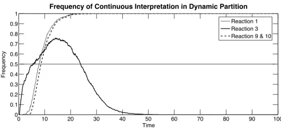
Figure 2.2 explains these results by showing the behavior of the dynamic partioning strategy in this example. On the long time horizon, the dynamic strategy interprets

(40)

reactions {1, 9, 10}, i.e., the production and reversible dimerization of protein M, as continuous and the other ones as stochastic. However, on the first 7 units of time, the dynamic strategy applies a completely different choice, with stochastic interpretation for those reactions and reaction 3, the RNA production, continuous. Then, for a transient time of around 20 units, reactions{1, 3, 9, 10} are mainly continuous with a decreasing frequency for reaction 3.

0 10 20 30 40 50 60 70 80 90 100 0 0.1 0.2 0.3 0.4 0.5 0.6 0.7 0.8 0.9 1

Frequency of Continuous Interpretation in Dynamic Partition

Time

Frequency

Reaction 1 Reaction 3 Reaction 9 & 10

Figure 2.2: The frequency of each reaction being interpreted as continuous under dynamic partition strategy, over time horizon of 100 units, and calculated over 1000 simulations. Reactions not listed are never interpreted as deterministic during the simulation horizon.

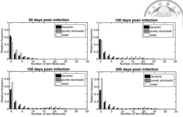
Example 2.5 Let us consider again the model of intracellular growth of bacterio-phage T7 of Example 2.2 with the static partitioning strategy of [4], noted_{{1, 2, 3, 4}} since the first four reactions are always stochastic and the last two ones always continuous, and with a different static partition_{{1, 3} in which only the first and} third reactions are stochastic, the others being continuous. For dynamic partition, the propensity threshold and the particle count threshold are set to be 10 (with n1= 10) and 5 (with n2= 5), respectively.

(41)

0 5 10 15 20 25 30 35 0 0.2 0.4 0.6 0.8 1 50 days post−infection

Number of tem Molecules

Relative frequency dynamic purely stochastic static 0 5 10 15 20 25 30 35 0 0.2 0.4 0.6 0.8 1 100 days post−infection

Relative frequency

dynamic purely stochastic static

Figure 2.3: Comparison of post-infection distributions of tem particle counts obtained at time= 50, 100, 150, 200 days, by stochastic, static hybrid and dynamic hybrid simulations (based on 1000 simulation runs of each strategy.)

Figure 2.3 depicts the relative frequencies of the numbers of tem molecules after 50, 100, 150, 200 days, obtained with that static partition, with the dynamic partitioning strategy, and with SSA. Each bar represents the relative frequency of tem molecule count falling in that region after certain amount of time. As can be clearly seen in the graph, bars of static partition deviate from those of purely stochastic simulation, while bars of dynamic partition are closer to the purely stochastic ones.

These observations can be made quantitative using statistical distances. Let us use the two sample Kolmogorov-Smirnov test as distance measure (KS distance) to compare the relative frequencies. Table 2.3 shows the KS distance between the distributions obtained by SSA and the static partitioning_{{1, 2, 3, 4} of [4], the static} partitioning _{{1, 3} and the dynamic partitioning respectively.}

(42)

2.4. Hybrid Boolean models

Post-infection Time (days) 50 100 150 200

KS distance SSA - static hybrid {1, 2, 3, 4} 0.0525 0.7145 0.8035 0.836 KS distance SSA - static hybrid _{{1, 3}} 0.3815 0.9225 0.624 0.6055

KS distance SSA - dynamic hybrid 0.0515 0.116 0.1485 0.161 Table 2.3: Post-infection distributions of tem molecules from simulations using different hybrid strategies compared to the reference fully stochastic model. Each row contains the outcome of applying two-sample Kolmogorov-Smirnov test on the distributions obtained from 1000 simulations using specified hybrid strategy and the reference fully stochastic model. The smaller the value, the more similar the two distributions involved. Distributions at four sampling points are used for comparison through the evolution of time, as listed in four corresponding columns.

By taking the particle count distribution of purely stochastic simulation as the reference, this example shows that the dynamic strategy always beats the static partition strategies and improves the accuracy of the simulation to a small distance from SSA along all time points.

2.4 Hybrid Boolean models

In this section we demonstrate how Boolean models can also be composed with continuous and even hybrid continuous-stochastic models in SBML.

2.4.1 Preprocessor for composing continuous and Boolean

models

In this section, we consider the composition of continuous reaction models with Boolean transition systems. One typical use of this form of composition is for modeling the interactions between gene expression and metabolism on different time scales. Gene networks can be modeled by simple Boolean regulatory networks

(43)

representing the on/off states of the genes and the possible transitions from one state to another, while metabolic networks are naturally modeled by chemical reactions with continuous semantics. Hybrid models of gene expression and metabolism can thus be naturally built as hybrid continuous-Boolean models, and analyzed and simulated as such.

A continuous-Boolean composition necessitates specifying:

• the link between the discrete/continuous variables and the Boolean variables, e.g. by fixing particle count or concentration threshold values,

• the relationship between the discrete logical time of the Boolean model and the continuous real time of the continuous reaction model, e.g. by adding delays on Boolean transitions,

• the integrity constraints between both dynamics.

There is currently no general method for these tasks. Our high-level interface takes as input

1. a reaction model that accommodates both stochastic and continuous semantics, 2. a Boolean transition system,

3. an interface specifying for each Boolean transition, the triggers and actions on the reaction model variables,

and produces as output a system of reactions and events which synchronize the execution of both input models.

(44)

2.4. Hybrid Boolean models

2.4.2 Hybrid composition of continuous-Boolean models

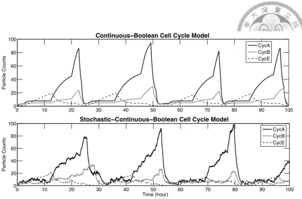
In [71], Singhania et al. have proposed a simple hybrid model of the mammalian cell cycle regulation. This cell cycle model of low dimension has been evaluated in terms of flow cytometry measurements of cyclin proteins in asynchronous populations of human cell lines. The few kinetic constants in the model are easier to estimate from the experimental data than the numerous kinetic constants of a single large ODE model.

In this model, cyclin abundances are tracked by piecewise linear continuous equations for cyclin synthesis and degradation. Cyclin synthesis is regulated by transcription factors whose activities are represented by discrete variables (0 or 1) and likewise for the activities of the ubiquitin-ligating enzyme complexes that govern cyclin degradation. The discrete variables change according to a predetermined sequence, with the times between transitions determined by the amount of cyclin presented as well as exponentially distributed random variables.

This model can be reconstructed using our interface as the hybrid composition of a purely continuous reaction model of cyclin activation and degradation, with a Boolean model of cell cycle phase transitions. We provide here the real examples and thus the ASCII syntax for the Biocham constructs described in Section 2.1.1. Beside the syntax introduced before, the present command specifies the initial concentration, and the macro command defines a function that makes the reaction rates dependent on the value of boolean variables, as specified in the original article.

The inputs are:

(45)

progressing continuous behavior: 1 % Initial C o n d i t i o n s 2 present ( CycA , 1) . 3 present ( CycB , 1) . 4 present ( CycE , 1) . 5 6 % R e a c t i o n Rules 7 k_sa for _ = > CycA . 8 MA ( k_da ) for CycA = > _ . 9

10 k_sb for _ = > CycB . 11 MA ( k_db ) for CycB = > _ . 12

13 k_se for _ = > CycE . 14 MA ( k_de ) for CycE = > _ . 15

16 macro ( k_sa , 5+6* B_tfe +20* B_tfb ) . 17 macro ( k_sb , 2.5+6* B_tfb ) .

18 macro ( k_se , 0.02+2* B_tfe ) .

19 macro ( k_da , 0 . 2 + 1 . 2 * B _ c d c 2 0 a +1.2* B_cdh1 ) . 20 macro ( k_db , 0 . 2 + 1 . 2 * B _ c d c 2 0 b +0.3* B_cdh1 ) . 21 macro ( k_de , 0 . 0 2 + 0 . 5 * B_scf ) .

2. the Boolean transition system of the cell cycle progression, which is given in [71] as the following limit cycle of state transitions. The add boolean state command defines a numbered state, and associates the boolean variables true in that state; the add boolean transition command defines a named transition between two states. Here is an excerpt of the file:

1 % States and c o r r e s p o n d i n g active boolean species 2 a d d _ b o o l e a n _ s t a t e (1 , [ B_cdh1 ]) . 3 a d d _ b o o l e a n _ s t a t e (2 , [ B_tfe , B_cdh1 ]) . 4 a d d _ b o o l e a n _ s t a t e (3 , [ B_tfe ]) . . . . 1 s e t _ i n i t i a l _ b o o l e a n _ s t a t e (1) . 2 3 % T r a n s i t i o n s between states 4 a d d _ b o o l e a n _ t r a n s i t i o n ( T12 , 1 , 2) .