HAL Id: ensl-00362174
https://hal-ens-lyon.archives-ouvertes.fr/ensl-00362174
Submitted on 17 Feb 2009
HAL is a multi-disciplinary open access
archive for the deposit and dissemination of
sci-entific research documents, whether they are
pub-lished or not. The documents may come from
teaching and research institutions in France or
abroad, or from public or private research centers.
L’archive ouverte pluridisciplinaire HAL, est
destinée au dépôt et à la diffusion de documents
scientifiques de niveau recherche, publiés ou non,
émanant des établissements d’enseignement et de
recherche français ou étrangers, des laboratoires
publics ou privés.
Testing fractal connectivity in multivariate long memory
processes
Herwig Wendt, Antoine Scherrer, Patrice Abry, Sophie Achard
To cite this version:
Herwig Wendt, Antoine Scherrer, Patrice Abry, Sophie Achard. Testing fractal connectivity in
multi-variate long memory processes. ICASSP 2009 - IEEE International Conference on Acoustics, Speech
and Signal Processing, Apr 2009, Taipei, Taiwan. �ensl-00362174�
TESTING FRACTAL CONNECTIVITY IN MULTIVARIATE LONG MEMORY PROCESSES
H. Wendt, A. Scherrer, P. Abry,
Physics Dept., ENS Lyon, CNRS,
46, Allée d’Italie 69364 Lyon Cedex 07, France
[email protected]
S. Achard
GIPSA Lab, UMR CNRS 5216,
Grenoble, France
[email protected]
ABSTRACT
Within the framework of long memory multivariate processes,
fractal connectivityis a particular model, in which the low frequen-cies (coarse scales) of the interspectrum of each pair of process com-ponents are determined by the autospectra of the comcom-ponents. The underlying intuition is that long memories in each components are likely to arise from a same and single mechanism. The present con-tribution aims at defining and characterizing a statistical procedure for testing actual fractal connectivity amongst data. The test is based on Fisher’s Z transform and Pearson correlation coefficient, and an-chored in a wavelet framework. Its performance are analyzed theo-retically and validated on synthetic data. Its usefulness is illustrated on the analysis of Internet traffic Packet and Byte count time series.
Index Terms— Fractal connectivity, Long memory, Wavelet transform, Statistical test, Internet traffic
1. INTRODUCTION
Sensor network deployment is nowadays common for system moni-toring in many different applications, such as medicine, biology, en-vironment, . . . to name but a few (cf. e.g., [1] and reference therein). Therefore, data to be analyzed often consist of multivariate time se-ries, conveying in a potentially redundant and correlated manner the information practitioners are interested in. Measuring the amount of information shared amongst such data, or their (inter-)correlation levels (or functions), are often key issues in multivariate data anal-ysis and processing. Moreover, in a large number of applications, the time series to be analyzed are characterized by long range de-pendence [2]: Their autocorrelation functions have extremely slow (algebraic power law type) decay, significantly complicating analy-ses aiming at establishing whether - and to which extent - the dif-ferent time series embody identical or complementary information. A fundamental question arising from the analysis of long memory multivariate data is whether there is a unique mechanism in the sys-tem controlling long range dependence on the different data compo-nents, or whether there are different mechanisms at work, producing
unconnectedlong memory properties. The goal of the present con-tribution is to propose a statistical test providing practitioners with elements of answer to such questions. Our study is based on the so called fractal connectivity model, recently introduced in [3] and consisting of multivariate long memory time series (recalled in Sec-tion 2): Fractal is used to refer to long memory while
connectiv-ityimplies that the interspectrum is proportional to the product of the autospectra in the limit of coarse analysis scales (equivalently, low frequencies), i.e, the coherence function goes to a non zero
con-stant in the limit|f| → 0. It is now well-known that long range
dependence phenomena are relevantly and accurately analyzed in a wavelet framework [4] (briefly re-sketched in Section 3). Therefore,
to test the fractal connectivity model, we propose a statistical pro-cedure, based on the discrete wavelet transform coherence function and Fisher’sZ transform. It is explained and defined in Section 4. Its performance are devised analytically and validated numerically by application to synthetic bivariate long memory time series with and without fractal connectivity (cf. Section 5). It is then applied to Internet traffic packet and byte count time series, collected very recently on a major transpacific backbone (cf. Section 6).
2. BIVARIATE FRACTAL CONNECTIVITY
Long memory. Long memory(LM), or long range dependence,
is defined, for a processX, as a power law behavior of its spectrum ΓX(f ) at the origin [2]:
ΓX(f )∼ C|f|−α,|f| → 0, with 0 < α < 1. (1)
This property has been widely observed for many different data in various research domains and its relevant analysis is important be-cause it is known to strongly impair parameter estimation and to de-grade the performance of a system, e.g., the amount of buffer needed on an Internet link.
Bivariate long memory model. For simplicity of notation, and
without loss of generality, we restrict presentation here to the bi-variate case only. The proposed test can be straightforwardly ex-tended to the multivariate case by considering time series pairwise. LetZ = {Z(t)}t∈Z ={[X(t), Y (t)]}t∈Zbe a real-valued
bivari-ate discrete time series. Following [3],Z is called a bivariate long
memory processwith parametersαX,αY,α1andα2if itsN -th
or-der difference process ˜Z(t) = δNZ(t) is stationary and has spectral and inter-spectral densities (−π ≤ f ≤ π), where the Ω·consist of
arbitrary positive multiplicative factors: ΓW˜(f ) = ΩW˜ ˛ ˛ ˛1 − e −jf˛˛ ˛ −2αW Γ∗W˜(f ), W = X or Y(2) ΓX ˜˜Y(f ) = Ω12 “ 1− e−jf”−α1“1− ejf”−α2Γ∗12(f ). (3)
The parametersα(·)are confined to the range [0, 0.5]. The
func-tionsΓ∗
(·)(f ) are non-negative, symmetric, with limit 1 at the origin,
hence modeling short memory (SM) properties at high frequencies, without affecting the spectral densities around the origin. Let us
defineαXY = α1 + α2. By definition, the coherence function:
CX ˜˜Y(f ) =
|ΓX ˜˜Y(f )| √Γ
˜ X(f )ΓY˜(f )
, has to be between 0 and 1. Also, it be-haves asymptotically, in the limitf→ 0, as [3]:
CX ˜˜Y(f )∼f →0C0|f|−(αXY−αX−αY). (4)
This shows that the model is well defined only ifαXY ≤ αX+ αY
and thatC0 =|Ω12|/pΩX˜ΩY˜ is a constant, controlling the global
Fractal connectivity. Fractal connectivityis theoretically defined as the special case whereC0 6= 0 and CX ˜˜Y(f ) exactly reduces to
a non-zero constant over a range of coarse scales (low frequencies). Equivalently, this implies,C06= 0 and:
αXY = αX+ αY. (5)
Essentially, the test described below aims at testing this equality. The intuition underlying fractal connectivity is that a same and single mechanism in the system uniquely controls the independent and joint LM properties of the multivariate data components. This test can hence avoid practitioners the burden of erroneously searching for different causes for LM.
3. DISCRETE WAVELET TRANSFORM
Discrete wavelet transform. A mother waveletψ0(t) is a
refer-ence pattern with narrow supports in both time and frequency do-mains. It is characterized by its number of vanishing momentNψ ≥
1:∀k = 0, 1, . . . , Nψ− 1, R Rt kψ 0(t)dt≡ 0 and R Rt Nψψ 0(t)dt6=
0. Also, it is such that the{ψj,k(t) ≡ 2−j/2 ψ0(2−jt− k), j ∈
N, k ∈ N} form a basis of L2(R). The discrete wavelet transform (DWT) coefficients ofX are defined as: dX(j, k) =hX, ψj,ki. For
further details, readers are referred to e.g., [5].
Stationary processes. Let ˜X and ˜Y denote second order station-ary processes. It is straightforward to show that [4]:
Ed˜ W(j, k) 2=Z Γ ˜ W(f )2 j |Ψ0(2jf )|2df, ˜W = X or Y,(6) Ed˜ X(j,k)dY (j,k)˜ = Z ΓX ˜˜Y(f )2 j |Ψ0(2jf )|2df, (7)
whereΨ0stands for the Fourier transform ofψ0and E for the
math-ematical expectation. Following [4, 6], relevant wavelet based esti-mators for the auto- and inter-spectra of ˜X and ˜Y are defined as:
SW(2j) = 1 nj nj X k=1 dW(j, k)2, W = ˜X or ˜Y , (8) SX ˜˜Y(2 j) = 1 nj nj X k=1 dX˜(j, k)dY˜(j, k), (9)
wherenjis the number of coefficients available at scale2j.
Quali-tatively, the scale2jacts as the inverse of the frequency,f∼ f0/2j,
withf0a constant depending onψ0.
Bivariate long memory processes. For bivariate LM processes
Z, on condition that Nψ > N , the wavelet coefficients dXanddY
at scalej form stationary sequences, and Eqs. (6-7) translate to: EdX(j, k)2 ∼ cX22j(αX+N ), Ed
Y(j, k)2 ∼ cY22j(αY+N ) and
EdX(j, k)dY(j, k)∼ cXY22j(αXY+N ), when2j → +∞. Also, it has been proven that thedX(j, k) and dY(j, k) are freed from LM,
so that the time averagesSX, SY, SXY provide efficient and robust
estimators of the spectra ofZ, and of their power law exponents [4]. This implies that the wavelet coherence function [6] behaves, in the limit of coarse scales, as (withγ0= cXY/√cXcY):
ˆ
γXY(2j) = SXY(2
j)
pSX(2j)SY(2j)
≃ γ02j(αXY−αX−αY). (10)
Fractal connectivity. If fractal connectivity, Eq. (5), is valid, Eq. (10) above implies thatγˆXY(2j) takes a quasi constant non zero
value over a range of coarse scales2j
≥ 2J1: ˆ
γXY(2j)≃ γ06= 0, (11)
while it decreases to0 as γ02j(αXY−αX−αY)otherwise. This serves
as the key ingredient for the design of a test for fractal connectivity. 4. TESTING FRACTAL CONNECTIVITY
Test formulation. TheˆγXY(2j) can be read as the Pearson
prod-uct-moment correlation coefficient of the seriesdX(j,·) and dY(j,·).
It is known that, for many distributionsF , dX(j,·)∼ F , the Fisher’sd
Z statistic ˆzXY(2j) of ˆγXY(2j) is asymptotically Normal (e.g. [7]):
ˆ zXY(2j) = 1 2ln 1 + ˆγXY(2j) 1− ˆγXY(2j) d ∼ N (zXY(2j), σ(2j)), (12) withzXY(2j) = 12ln1+γXY(2 j) 1−γXY(2j) and varianceσ 2(2j) = 1 nj−3, whereγXY(2j) = EdX(j, k)dY(j, k)/pEdX(j, k)2EdY(j, k)2.
Therefore, testing fractal connectivity can be formulated as a test of the equality of means of Gaussian r.v.s with known but different variances, i.e., of the null hypothesis:
H0: zXY(2J1)≡ zXY(2J1+1)≡ · · · ≡ zXY(2J2), (13)
where the scale rangej ∈ [J1, J2] is discussed below. Let J =
J2− J1+ 1. The test statistic for the UMPI test of equality of means
of Gaussian r.v.s is given by [8]: ˆ VJ = J2 X j=J1 1 σ2(2j) zˆXY(2 j )− PJ2 j=J1zˆXY(2 j)/σ2(2j) PJ2 j=J11/σ2(2j) !2 . (14) UnderH0, idealizing the quasi-decorrelation of the wavelet
coeffi-cient into exact independence [4], one expects ˆVJto follow aχ2(J−1)
distribution. Consequently, the(1− α) significance test for fractal connectivity can be formulated as:
ˆ
dJ = 1 if ˆVJ > Cχ, ˆdJ = 0 otherwise, (15)
whereCχis the upper(1− α) percentile of the χ2(J−1)distribution.
Similarly, the p-value of the observed test statistic ˆVJ is given by:
ˆ
pJ= 1− ˜χ2(J−1)( ˆVJ), where ˜χ2(J−1)denotes the cumulativeχ2(J−1)
distribution function.
Power of the test. WhenH0is not true, ˆVJfollows a non-central
χ2(J−1),VJ distribution, where VJ is given by Eq. (14) withz(j) replacingz(j). This enables to evaluate explicitly the power of theˆ test against a specific alternative hypothesisαXY − αX− αY < 0.
Scale range. Selecting the range of scalesj ∈ [J1, J2] where
to perform the test results from a standard trade-off:J1needs to be
chosen large enough so that SM (controlled by theΓ∗(·)) no longer
contribute (Type I error); however a too largeJ1decreases effective
sample size and the power of the test (Type II error).J2is naturally
limited by the available sample size (J2≃ log2n).
5. TEST PERFORMANCE
Numerical simulations. To evaluate the test performance, we
apply it to a large numberNM C = 1024 of realizations of length
n = 218of Gaussian bivariate 2nd order stationary (henceN = 0,
cf. Section 2) long memory processes, with prescribed auto- and inter-spectra according to Eqs. (2-3), implemented by ourselves fol-lowing Chambers’ algorithm [9]. The constantC0 is varied within
0.5≤ C0 ≤ 0.9, implying a significant global correlation between
X and Y , be they fractally connected or not. Parameters are set to
5 10 −1.5 −1 −0.5 0 0.5 j log 2|γXY(2 j )| 5 10 0.8 1 1.2 1.4 j z XY(2 j ) 5 10 −1 0 1 2 3 j log 2SX(2 j ) 5 10 −5 0 5 10 j log 2SY(2 j ) 5 10 −2 0 2 4 6 j log 2|SXY(2 j )|
Fig. 1: Wavelet spectra. Average (and95% CI for) wavelet
spec-tra and inter-spectrum ofX and Y (top), wavelet correlation and
FisherZ statistics (bottom) under H0without SM (C0= 0.7).
5 10 −6 −4 −2 0 2 j log2|γXY(2j)| 5 10 −0.5 0 0.5 1 1.5 j zXY(2j) 5 10 −1.5 −1 −0.5 0 j log 2|γXY(2 j )| 5 10 0 0.5 1 1.5 2 j z XY(2 j )
Fig. 2: Short memory and alternative hypothesis. Average (and
95% CI for) wavelet correlation (left column) Fisher’s Z statistic (right column) as a function of scales (C0 = 0.7) under H0 with
ARMA(1,1) SM (top) and underH1(bottom,αXY = 0.2).
αXY is varied from0 to αX+ αY = 0.4, so as to evaluate test
pow-ers. Short memory (SM) properties are modeled with ARMA(1,1)
processes (parameters{0.4, −0.3} for X and {−0.2, 0.1} for Y ).
The significance level is set toα = 0.1. Test performance are as-sessed by the mean rejection rates ¯dJ = ˆEM CdˆJand mean p-values
¯
pJ = ˆEM CpˆJ, where ˆEM C stands for the mean overNM CMonte
Carlo realizations: Ideally, underH0, ¯dJshould reproduce the
pre-set significance levelα, whereas the p-value should be uniformly distributed on[0, 1], hence ¯pJshould equal0.5; Under H1, the test
should rejectH0, hence the larger (smaller) ¯dJ(¯pJ), the better.
Wavelet spectra and coherence, FisherZ statistics. Fig. 1 shows,
underH0, the average over realizations (and corresponding 95%
asymptotic confidence intervals (CI)) of the (log of the absolute
val-0 10 20 30 0 0.05 0.1 χ2 J−1 V J Cχ 0 25 50 0 0.05 0.1 χ2 (J−1),V J χ2 J−1 V J Cχ
Fig. 3: Test statistic. Histogram of test statistic ˆVJ(points,C0 =
0.7) and the corresponding theoretical distribution (line), under H0
(left) andH1 (right,αXY = 0.2). The vertical line indicates the
10% significance critical valueCχ.
[J1, J2] = [7, 13] - 10% significance
Test decisions - mean rejection rates ¯dJ(in%)
αXY 0.4 0.35 0.3 0.25 0.2 C0= 0.5 9.4 22.7 42.9 54.9 56.8 C0= 0.7 10.3 51.9 83.0 89.2 89.3 C0= 0.9 8.7 99.3 99.9 99.9 99.9 Mean p-valuep¯J αXY 0.4 0.35 0.3 0.25 0.2 C0= 0.5 0.51 0.38 0.25 0.18 0.16 C0= 0.7 0.50 0.18 0.06 0.04 0.04 C0= 0.9 0.50 0.00 0.00 0.00 0.00
Table 1: Test performance. Mean test decisions (top) and
p-values (bottom) for different p-values ofC0andαXY.
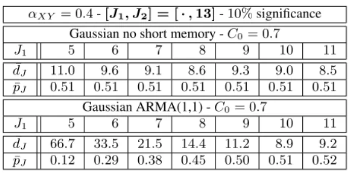
αXY = 0.4 - [J1, J2] = [ · , 13] - 10% significance
Gaussian no short memory -C0= 0.7
J1 5 6 7 8 9 10 11 ¯ dJ 11.0 9.6 9.1 8.6 9.3 9.0 8.5 ¯ pJ 0.51 0.51 0.51 0.51 0.51 0.51 0.51 Gaussian ARMA(1,1) -C0= 0.7 J1 5 6 7 8 9 10 11 ¯ dJ 66.7 33.5 21.5 14.4 11.2 8.9 9.2 ¯ pJ 0.12 0.29 0.38 0.45 0.50 0.51 0.52
Table 2: Scale range. Mean test decisions (in%) and p-values
for different values ofJ1, without (top) and with (bottom) SM.
ues of the) wavelet (inter-)spectra (top) and coherence, and Fisher’s Z statistics (bottom), when no SM are present (i.e., Γ∗(·) ≡ 1). It
indicates that the estimatesˆγXY(2j) and ˆzXY(2j) are quasi
con-stant over the entire range of available scales2j, as predicted by the
model. Fig. 2 illustratesˆγXY(2j) and ˆzXY(2j) under H0 (C0 =
0.7) when SM are present (top row), and under H1 (bottom row,
αXY = 0.2). The plots indicate that: i) Under H0, the existence of
SM has a clear impact on fine scales (below2j≤ 2J1 = 27). Yet,
at coarse scales, bothγˆXY(2j) and ˆzXY(2j) are quasi-constant; ii)
UnderH1, bothγˆXY(2j) and ˆzXY(2j) display a significantly
non-constant behavior with scales2j. These preliminary investigations
clearly validate the test as formulated in Eqs. (13-15).
Test performance: Significance. Tab. 1 summarizes mean test
decisions and p-values whenαXY andC0are varied and no SM is
present. UnderH0(αXY = 0.4, left column), the targeted 10%
sig-nificance level is closely reproduced and mean p-values are close to the expected value0.5, regardless of the precise value of C0,
indicat-ing that the test statistic ˆVJEq. (14) accurately follows the predicted
χ2
(J−1)distribution. This is further confirmed in Fig. 3 (left),
show-ing the histogram of ˆVJunderH0.
Test performance: Power. Tab. 1 (col. 3-6) clearly indicates that the test is powerful in rejectingH0whenαXY < αX+ αY and an
alternative hypothesis is true: With increasing discrepancy between αXY andαX + αY, mean rejection rates (p-values) increase
(de-crease). Also, the largerC0, the more powerful the test: For large
global correlationC0 = 0.9, the test rejects fractal connectivity with
probability close to1 already for discrepancy in exponents αXY and
αX+ αY as small as0.05. Fig. 3 (right) confirms that the test
statis-tic ˆVJ closely follows the predicted non centralχ2(J−1)distribution
0 50 100 Packet X 0 1 2 3x 10 4 Byte Y
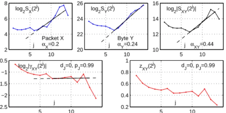
Fig. 4: Internet time series. Packet (left) and byte (right) counts as functions of time,∆0= 10ms. 5 10 −2.5 −2 −1.5 −1 −0.5 j log 2|γXY(2 j )| d J=0, pJ=0.99 5 10 0.2 0.4 0.6 0.8 1 j z XY(2 j ) d J=0, pJ=0.99 5 10 2 4 6 8 j log2SX(2j) Packet X αX=0.2 5 10 20 22 24 26 j log2SY(2j) Byte Y αY=0.24 5 10 10 12 14 16 j log2|SXY(2j)| αXY=0.44
Fig. 5: Wavelet spectra. Wavelet (inter-)spectra for Packet and
byte counts (top), wavelet coherence andZ statistics (bottom).
Scale range and short memory. Tab. 2 compares the impact of
the choice ofJ1 on test performance underH0, without (top) and
with (bottom) SM. Without SM, the targeted10% significance level (and the correspondingp = 0.5 average p-value) are systematically well reproduced, regardless of the choice ofJ1. In contrast, with
SM, the scale range must be restricted to coarse scalesj≥ J1= 9 to
reproduce nominal performance, resulting in less powerful tests and increased difficulty in rejecting the fractal connectivity hypothesis.
6. INTERNET TRAFFIC TIME SERIES
Internet monitoring and security nowadays constitute major tasks and challenges, often achieved by means of traffic flows statistical characterization. Commonly, Internet traffic is analyzed as aggre-gated time series, consisting of either IP packet (Pkt) or bytes (Byt) counts within bins of selected duration∆0. It is naturally suspected
that such time series should be correlated but their precise inter-relation is still an open debate. Moreover, Internet traffic is well known to be characterized by a strong LRD property [4], and we in-tend here to illustrate the usefulness of the proposed test to analyze LRD jointly in Pkt or Byt counts and hence to contribute to the on-going debate: Should practitioners concentrate on the analysis of Pkt or Byt counts? Data analyzed are part of the MAWI data set (1GB public repository available at http://mawi.wide.ad.jp/, cf. [10]). Results are reported here for data collected on March 3rd, 2006, between 7.30am and 7.45am (Tokyo time), on a transpacific OC3 backbone link (time series shown in Fig. 4). Fig. 5 indi-cates that both Pkt and Byt counts present LRD, at coarse scales 2j
≥ 2J1 = 27, i.e., roughly, for time lags larger than0.125s. It also reveals a power law behavior for the wavelet inter-spectrum and a quasi-constant wavelet coherence function at coarse scales. When applied to data, the test (with a10% targeted significance level) val-idate the hypothesis of fractal connectivity, with an output p-value ofp = 0.99, indicating that data show absolutely no evidence for rejection. Equivalent results are obtained from numerous different time series within the MAWI data sets. This leads to conclude that
LRD in Pkt and Byt time series result from a single and same net-work mechanism and are hence not created from different netnet-work sources. However, for a number of data, wavelet inter-spectra differ significantly from the one shown here (while individual auto spectra do present LRD). When applied, the test indicates no correlation at coarse scales and significantly rejects fractal connectivity, suggest-ing that LRD in Pkt and Byt may result from different and indepen-dent causes. Manual inspections tend to indicate that such cases are related to the occurrence of anomalies in the traffic, be they legit-imate or not. This requires further validation and is under current investigation. This opens new perspectives for Internet traffic moni-toring and for automated anomaly detection, where inter-spectra are rarely considered, despite the multivariate nature of traffic data.
7. DISCUSSION AND CONCLUSION
A statistical test for fractal connectivity in bivariate time series has been defined, analyzed and assessed. Its extension to multivariate data is straightforward, by considering each pair of data components. The test relies on wavelet based estimations of the autospectra, in-terspectra and coherence functions of the data. It has been shown to present satisfactory practical performance. To our knowledge, this is the first procedure for testing joint long memory properties of mul-tivariate data practically available in the literature. It provides prac-titioners with elements of answers to questions regarding the inde-pendence or not of the mechanisms at work in the production of the data, notably of their long range dependence property. Preliminary attempts for the analysis of Internet traffic and various biological and biomedical data indicate promising perspectives.
8. REFERENCES
[1] Z.-Q. Luo, M. Gastpar, J. Lui, and A. Swami, “Distributed sig-nal processing in sensor networks,” IEEE Sigsig-nal Proc. Mag., vol. 23, no. 4, pp. 14–15, 2006.
[2] J. Beran, Statistics for Long-Memory Processes, Chapman & Hall, 1994.
[3] S. Achard, D.S. Bassett, A. Meyer-Lindenberg, and E. Bull-more, “Fractal connectivity of long-memory networks,” Phys.
Rev. E, vol. 77, no. 3, pp. 036104, 2008.
[4] P. Abry, R. Baraniuk, P. Flandrin, R. Riedi, and D. Veitch,
“Multiscale nature of network traffic,” IEEE Signal Proc.
Mag., vol. 19, no. 3, pp. 28–46, 2002.
[5] S. Mallat, A Wavelet Tour of Signal Processing, Academic Press, San Diego, CA, 1998.
[6] B. Whitcher, P. Guttorp, and B. D. Percival, “Wavelet analysis of covariance with application to atmospheric time series,” J.
Geophys. Res. [Atmos.], vol. 105, pp. 14941–14962, 2000.
[7] D.L. Hawkins, “Usingu statistics to derive the asymptotic
distribution of Fisher’sz statistic,” American Statistical
Asso-ciation, vol. 43, no. 4, pp. 235–237, 1989.
[8] E.L. Lehmann, Testing Statistical Hypotheses, Wiley, New York, 1959.
[9] M.J. Chambers, “The simulation of random vector time series with given spectrum,” Mathematical and Computer Modelling, vol. 22, no. 6, pp. 1–6, July 1995.
[10] K. Cho, K. Mitsuya, and A. Kato, “Traffic data repository at the WIDE project,” in USENIX 2000 Annual Technical