HAL Id: insu-02186326
https://hal-insu.archives-ouvertes.fr/insu-02186326
Submitted on 17 Jul 2019
HAL is a multi-disciplinary open access
archive for the deposit and dissemination of
sci-entific research documents, whether they are
pub-lished or not. The documents may come from
teaching and research institutions in France or
abroad, or from public or private research centers.
L’archive ouverte pluridisciplinaire HAL, est
destinée au dépôt et à la diffusion de documents
scientifiques de niveau recherche, publiés ou non,
émanant des établissements d’enseignement et de
recherche français ou étrangers, des laboratoires
publics ou privés.
Toward resolving small-scale structures in ionospheric
convection from SuperDARN
R. André, J.-P. Villain, Catherine Senior, Laurent Barthès, C. Hanuise,
Jean-Claude Cerisier, A. Thorolfsson
To cite this version:
R. André, J.-P. Villain, Catherine Senior, Laurent Barthès, C. Hanuise, et al.. Toward resolving
small-scale structures in ionospheric convection from SuperDARN. Radio Science, American Geophysical
Union, 1999, 34 (5), pp.1165-1176. �10.1029/1999RS900044�. �insu-02186326�
Radio Science, Volume 34, Number 5, Pages 1165-1176, September-October 1999
Toward resolving small-scale structures in ionospheric
convection from SuperDARN
R. Andre, • J.-P. Villain, 1 C. Senior,
2 L. Barthes, 2 C. Hanuise,
a
J.-C. Cerisier,
2 and A. Thorolfsson
2
Abstract. The combination of radial velocities measured by a pair of Super Dual Auroral
Radar Network (SuperDARN) HF coherent radars gives, in their common field of view,
the velocity vectors in a plane perpendicular to the magnetic field. The standard merging is based on a natural grid defined by the beam intersections, which provides a resolution
varying between 90 and 180 km (depending upon the distance to the radars). This allows the description of structures with a typical scale size (L) of the order of 500 km. The
present study is devoted to a merging method which takes advantage of individual radar
grids to enhance the resolution (L • 200 km). After a brief description of the standard
merging method, we define the high-resolution grid and discuss the potential problems which have to be overcome. The first problem concerns the localization of the scattering volume, whereas the second one deals with the independence of the velocity vectors. These
two limitations have been addressed in previous studies [Andrd et al., 1997; Barthes et al., 1998]. In the method proposed here, several velocity vectors are determined at each
grid point, from which the selection is made by using the hypothesis of minimization of the divergence magnitude. The selected map is the one which minimizes the divergence. The performances are tested and compared to the standard merging algorithm through simulated double vortices. Finally, we apply this method to real data, and show, through
two examples, its ability to describe small-scale structures (L m 200 kin).
1. Introduction
The combination of radial velocities measured by
a pair of HF coherent radars gives, in their common
field of view, the velocity vectors in a plane perpen-
dicular to the magnetic field. Super Dual Auroral
Radar Network (SuperDARN) radars [Greenwald et al., 1995a] are able to determine the radial veloci-
ILaboratoire de Physique et Chimie de
l'Environnement, CNRS, Orl6ans, France.
2Centre d'Etude des Environnements Terrestres et
Plan6taires, CNRS, Saint-Maur, France.
3Laboratoire
de Sondage
Electromagn6tique
de
l'Environnement Terrestre, CNRS, Universit6 de Toulon,La Garde, France.
Copyright 1999 by the American Geophysical Union.
Paper number 1999RS900044.
0048-6604/99/1999RS900044511.00
ties in 16 different directions and 70 range gates. In
the basic mode of operation the radial resolution is
45 km. Currently, velocity vectors are computed at the natural grid points defined by the beam intersec-
tions. The associated velocity map thus contains 256 potential vectors. This technique leads to a spatial
resolution varying between 90 and 180 km depending
upon distance to the radar.
These maps have been used for studies of large-
scale structures (characteristic scale length approxi- matively equal to 500 km) in the ionospheric convec- tion, such as vortices [Bristow et al., 1995; Green-
wald et al., 1995b, 1996], but they cannot describe smaller-scale structures (L • 200 km). There is a
need to resolve these small-scale structures, which
are thought to be associated with reconnection at
the cusp [Rodger and Pinnock, 1997] or on the night- side, in relation with substorm activity [Yeoman and Luhr, 1997; Lewis et al., 1997].
The purpose of this paper is to present an algo- rithm which provides a high spatial resolution map of
1166 ANDRI• ET AL.: SUPERDARN HIGH-RESOLUTION MAPPING
the ionospheric convection. This spatially improved resolution is based on a grid determined by the ra- dial resolution of the measurements, i.e., 45 km in the standard radar operating mode. In section 2, we briefly review the standard method presently used to compute velocity vector maps with one pair of radars. We discuss the advantages and limitations of this grid and the intrinsic difficulties related to a high- resolution grid. We then discuss the approach used to overcome these problems and present the global analysis conducted to compute this high-resolution map. Using simulated data, we illustrate the perfor-
mances of this technique and demonstrate its ability
to describe structures with a typical scale length of the order of 200 km. In section 3, this method is applied to real SuperDARN data containing a con-
vection reversal and a vortex. We demonstrate that
the vector maps preserve the resolution of the radial velocity maps of each radar.
2. Toward a High-Resolution Map
Before presenting the high-resolution merging al- gorithm, we briefly review the method used rou- tinely for SuperDARN data, which was described
by Cerisier and Senior [1994]. We then discuss
the problems arising from the choice of the high- resolution grid.
2.1. Standard Merging
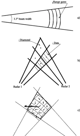
Before calculating vector velocities from the avail- able data set, a grid needs to be defined. Figure l a
represents the experimental data set: A radial veloc-
ity is measured in each elementary cell defined by a beam direction and a gate number. The dimension of a cell in the standard mode of operation is 45 km in range and variable in the transverse direction as a function of range.
2.1.1. The grid. The standard grid is defined by the intersection of radar beams from two radars, as shown in Figure lb. The common area of two
beams defines a "diamond." The radial velocities
falling into this diamond are averaged for each radar, and the mean velocity vector is computed from these two averaged radial velocities. Each radar being
scanned in 16 different directions, a two-dimensional map contains 256 potential velocity vectors. The
spatial resolution depends on the azimuthal separa-
tion between beams. As the azimuthal width of a
cell increases linearly with distance from the radar,
i Range gates a)
I Diamond A
b) Radar 1 Radar 2 c)Figure 1. Schematic view of (a) the experimental data set with several gates in one radar beam, (b) the standard merging grid, and (c) the high-resolution
grid.
the spatial resolution of this grid is not constant and
varies from about 60 km at 1000 km to about 150 km at 2500 km.
The main advantage of this grid is that the resolu-
tion takes into account the increase of the azimuthal
beam width with range. Therefore all velocity vec- tors are mutually independent. One radial velocity
measurement is used in only one diamond.
2.1.2. Velocity vector computation. The
first step in combining radial velocities to derive two-
dimensional vectors is to associate a diamond to each
ANDRt• ET AL.' SUPERDARN HIGH-RESOLUTION MAPPING 1167
SuperDARN radars are taking advantage of HF
wave refraction in the ionosphere in order to achieve
perpendicularity between the wave vector and the Earth's magnetic field lines in the auroral zone and polar cap. Without knowledge of the electron den- sity profile, radar echoes cannot be exactly localized. The simplest approximation is straight-line propaga,- tion to an assumed altitude. This technique has been
checked by Villain et al. [1984] and later by Baker et al. [1986]. Both groups of authors have estimated
the localization error, for an assumed altitude of 300 km, based on comparison with ray tracing in realis- tic ionospheric models. In each case the error was estimated to be smaller than 30-40 km, i.e., smaller or of the order of a standard range gate. This result has been confirmed on a statistical basis by Andr• et
al. [1997].
In the standard merging algorithm [Cerisier and Senior, 1994], an assumption for the propagation is used, based on the Breit and Tuve [1926] theorem. This theorem states that the time delay along the
real curved path in the ionosphere is equal to the
delay to a virtual altitude, situated vertically above the real height, and along a straight line in free space.
This theorem is subject to the condition that both rays have the same elevation angle at the radar site. Unfortunately, in the general case the elevation an- gle is not known, and a virtual altitude has to be as- sumed. In addition, the real altitude is never known
and also has to be assumed. The standard default values are 400 and 325 km for the virtual and real
heights, respectively.
From the time delay between transmission and re-
ception of the radar pulse, the backscatter area is then localized, and a diamond number is assigned to individual data points. Radial velocities from each radar measured in range gates belonging to the same diamond are then averaged. From the averaged ve- locities measured by each radar, the resultant veloc- ity for that diamond is calculated and is assigned to the "center" of the diamond, i.e., the point at which the centerlines of the two intersecting beams meet.
Whatever the hypothesis used to localize the scat- tering point, the expected error is much lower than
the mean spatial resolution of the grid. Through the
averaging process, the localization error on the radial
velocity is smoothed and does not affect significantly
the determination of velocity vectors. This means
that the standard grid is rather insensitive to local- ization errors.
In order to compute the velocity vector, one needs to know the magnetic field vector and the wave vec- tor inside the diamond. The magnetic field is given by the International Geomagnetic Reference Field
(IGRF) 95 magnetic field model. The velocity vector
is defined
by the set of equations
(1) where
•' is the
unit vector along the magnetic field, ki are the unitwave vectors transmitted from the radars I and 2,
and 1• are the measured Doppler velocities.
k•.V - V•
k•.V - V•
b.V - 0
These equations define the two components of the
velocity vector perpendicular to the magnetic field.
2.2. The High-Resolution Grid
We have defined a high-resolution grid using the intersection of measurement cells, as shown in Fig- ure lc. This figure shows the intersection of two dif- ferent beams, defining one standard diamond. Inside
this diamond are shown several measurement cells as
they are defined by the range gates. This configura- tion, i.e., 3x4 radar gates in a diamond, is typical of diamonds situated far from the radar, at a distance of the order of 2500 km. Figure lc clearly shows the increase in resolution to be expected from the use of the high-resolution grid, but it also illustrates one of
its limitations. As discussed previously, the localiza-
tion error can be of the order of the size of a grid
cell, and therefore it becomes necessary to study this
error in more detail.
In the high-resolution grid, the dimension of the
cells is constant whatever the distance to the radars.
The evaluation of the velocity vector in the cells sit-
uated at the same distance from a given radar is based on a single radial velocity measurement from
that radar. Therefore the vectors are interdependent.
This appears very clearly in Figure lc. This interde-
pendency increases with the distance to the radars.
This problem can be partly overcome by the use of a high-resolution spectral analysis which is able to ex- tract several velocities from a single autocorrelation
function (ACF). Following Barthes et al. [1998], the multiple signal classification (MUSIC) method has been selected.
1168 ANDR• ET AL.: SUPERDARN HIGH-RESOLUTION MAPPING
2.3. Localization Error
In order to estimate the error of localization, we
follow the method used by Andr• et al. [1997]. In
that paper, the authors have used a ray-tracing pro-
gram [Jones and Stephenson, 1975; Andr• et al., 1994] to localize radar backscatter in a statistical
sense. Using a series of representative ionospheric density profiles, the authors have estimated the local-
ization error introduced by the hypothesis considered
by Villain et al. [1984] and by Baker et al. [1986].
Their results are in agreement with these previous
studies.
Here we perform the same analysis in order to eval- uate the error introduced by the hypothesis used in the standard merging method, i.e., a straight- line propagation to a virtual altitude of 400 km fol- lowed by a projection to the real altitude of 325 km.
One thus estimates the field line on which backscat-
ter occurs. The group path required to probe the same magnetic field line is determined by ray trac- ing. Then the error is defined as the difference be-
tween these two values of the group path (the group
path associated with the propagation hypothesis is
substracted from the one associated with the simula- tion). This error is computed for several frequencies
and for 10 different ionospheric models, representa-
tive of the various electron density profiles charac- teristic of the high-latitude ionosphere. These sim- ulations suppose a direct propagation path in the magnetic meridian and with a backscatter originat-
ing from the F region [Andr• et al., 1997].
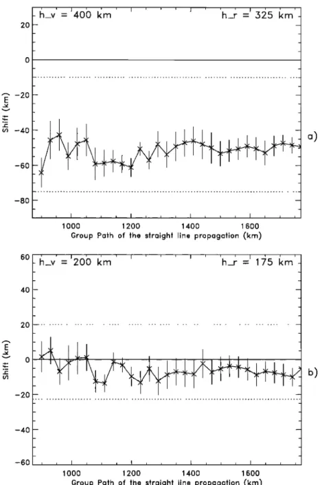
Figure 2a shows the error calculated along the propagation path and averaged over the radar fre-
quencies (11, 12, and 14 MHz) and over the 10 iono-
spheric density models. The error bars give the
variance of those mean values, and the dashed lines
show the maximum and minimum values obtained
throughout all the ray-tracing computations. This figure shows that the localization error is approxima- tively constant along the propagation path and that its mean value is of the order of 55 km, with a vari- ance of about 10 km. Figure 2b shows that this error can be minimized by changing the virtual altitude to 200 km and the real altitude to 175 km. In this case,
the maximum localization error is 20 km. As men-
tioned previously, these estimations do not take into account either strong electron density perturbation resulting from precipitations or the 1.5-hop propaga-
tion mode which is sometimes observed in the radar
data. Therefore, in the general case, we can at large
ranges consider that lowering the virtual height from
400 to 200 km reduces the localization error to the
order of magnitude of the spatial resolution in the
radial direction.
However, in contrast to the inscnsivity of the stan- dard merging grid to error, this localization error is critical in the case of the high-resolution grid, what-
ever the choice (within reasonable limits) of the vir-
tual and real heights. In order to consider all possible localization errors, several configurations should bc computed by shifting the data. The maximum shift amplitude considered here is of the order of the lo-
calization error found, i.e., one radial gate (45 kin).
In order to reduce the computation time, we make the hypothesis that the shift nccdcd is the same over the whole radar field of view, as observed in Figure 2. In conclusion, possible localization errors are taken into account by computing three different maps cor-
responding to three different shifts (+1, 0,-1 gate)
applied to all radial velocities.
2.4. High-Resolution Spectral Analysis
We have shown that the high-resolution grid im- plies that the same radial velocity measured by the radar in one range gate is used to compute several velocity vectors. Therefore the resulting vectors arc not totally independent. In order to reduce this ar- tificial smoothing, one has to increase the number of
radial velocities deduced from the radar data.
From the SuperDARN multipulse transmission sch- eme, the real-time data processing computes 17 points
of the complex autocorrelation function (ACF) of the
backscattered signal. As described by Villain et al.
[1987], the Doppler velocity is obtained from the fit of
the ACF phase, and the spectral width is obtained from the fit of the ACF power. The fitted model assumes a spectrum resulting from only one veloc- ity component corresponding to a linear variation of the ACF phase as a function of time. Barthes et al.
[1998] have shown that this is not always the case and
that the spectrum can include several components.
Schiffier et al. [1997] have indeed related multicom- ponent spectra to small scale vortices (10 kin) near
the projection of the low-latitude boundary layer. Multicomponent spectra can be used to reduce the interdependency of velocity vectors. However,
the resolution of the Fourier transform is not suf-
ficient, owing to the limited number of points in the ACF. On the contrary, high-resolution analysis can be achieved by the MUSIC method, which has
ANDRt• ET AL.' SUPERDARN HIGH-RESOLUTION MAPPING 1169
4oh I•m' ' ' ' ' ' ' 'h_; =' 5•5 I•m
20 "" -2.0
• -40
o) -60 1000 1200 14.00 1600Group Po4'h of The
60 40 20 -20 -40 -60 b) 1000 1200 1400 1 600
Group Pofh of fhe sfroighf line propogofion (km)
Figure 2. Localization
error along
the propagation
path for a virtual altitude
of (a) 400
km and (b) 200 km.been successfully applied to SuperDARN by Barthes et al. [1998]. These authors have shown that the method is very sensitive to data quality, and severe
criteria of applicability
have
been defined.
Owing
to
these selection criteria, however, the number of mul-ticomponent
spectra
is rather limited. For example,
when applying this analysis to a convection reversal where multicomponent spectra are expected close to the velocity shear, a significant enhancement of the probability of observing such spectra is effectively obtained, but with a maximum probability of only
1170 ANDRt• ET AL.: SUPERDARN HIGH-RESOLUTION MAPPING
In order to reduce the dependency between veloc-
ity vectors the MUSIC algorithm is applied to extract
the complete spectrum from each ACF. If a multi- component spectrum is obtained in one radar cell, a velocity vector is computed for each component.
Several vectors can therefore be obtained in one grid
point.
2.5. Selection Hypothesis
The solutions proposed above to solve the ques-
tions raised by the implementation of the high-resolu- tion grid lead to several possible velocity vectors
at one grid point (one gate shift and multicompo- nent spectra). Consequently, a selection criterion
has to be defined to choose among the several high- resolution maps obtained.
In the F region,•the
plasma
moves
in the E x B
direction, where E is the convection electric fieldand B is the Earth's magnetic field. This two- dimentional motion has been shown to be divergence-
free [e.g.,Ruohoniemi et al., 1989]. This hypothesis is
not scale dependent, and so is then true in the whole
auroral oval as well as in one grid cell. Nvectors
-
- 0
i=l
Taking into account this property, it is possible to select the configuration which minimizes the veloc- ity divergence. Such a velocity divergence can come
from experimental features (spatiotemporal integra-
tion in one radar gate, temporal variation of the con-
vection between beams, errors in the velocity deter-
mination,etc.). In order to avoid large and opposite divergences (large and opposite experimental errors)
we use the following selection criteria: Nvectors
minimum
(3)
The first step is to compute a reference map with
no multicomponent spectra and no shift due to lo-
calization errors. Then, for each global shift of the
map (0,-1, +1 range gate), the velocity divergence
is minimized by choosing between the various multi-
component spectra. Finally, we retain the map with
minimum divergence. At this point, we obtain a high-resolution map of the ionospheric convection, which takes into account possible localization errors, reduces the interdependency between velocity vec-
tors, and minimizes the magnitude of the velocity divergence.
2.6. Evaluation of the Method
Following the work of Wei and Lee [1990], Thorolf- sson [1996] has modeled the ionospheric signature of a flux transfer event (FTE). This consists of a double
convection vortex that travels at the same plasma ve- locity as in the central part of the vortex. Here we use
this model to reproduce a known signature and test the ability of the high-resolution method to resolve small-scale structures. In the following, the vortex is traveling through the radar field of view at a fixed
velocity of 1.5 km/s, typical of FTEs. By varying the
size of this simulated double vortex, it will be pos-
sible to determine the limits of the high-resolution method and compare with the results given by the standard mapping method.
In order to simulate the MUSIC results, each radar
range cell is subdivided into three parts, and the ra- dial velocities corresponding to the model are com- puted for each subdivided cell. We assume that the central part of the elementary cell is the radial veloc- ity deduced from the standard ACE analysis and that
the two others are the new radial velocities found by
the MUSIC method.
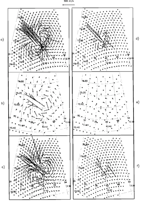
2.6.1. Scale length of 500 km. Figure 3a
shows the instantaneous velocity field of a structure
sitting in the middle of the radar field of view as pro- jected on the high-resolution grid before velocity pro- jection along the radar beams. The structure has a
scale length of 500 km. The points represent the grid
points, and the lines represents the velocity direction and amplitude. This map defines the reference map.
Figure 3a shows the well-defined double vortex struc-
ture, with plasma velocities of 1.5 km/s in the center.
Figure 3b shows the map deduced from the stan-
dard analysis and exhibits the same characteristics.
Figure 3c presents the map obtained with the high-
resolution method. The same structure is seen but
with a much better definition than in Figure 3b. The slight differences between Figures 3a and 3c are due to the fact that the structure is traveling through the radar fields of view, while projections along the radar
beams are made sequentially to mimic the real oper-
ation of the radars, which scan sequentially through all the beams. Therefore Figure 3c does not show the instantaneous signature of the FTE as in Figure 3a. From the similarities between Figure 3a and 3c, we can conclude that the high-resolution algorithm re-
ANDRI• ET AL.' SUPERDARN HIGH-RESOLUTION MAPPING 1171
o)
500 m/s ß
d)
Figure 3. Simulation
of a double
vortex
convection
pattern.
(a) Reference
double
vortex
with a scale
size
of 500
km. (b) Simulated
mee[surements
processed
with the standard
merg-
ing algorithm.
(c) Simulated
measurements
processed
with
the high-resolution
algorithm.
(d, e, f) Same
as Figure
3a, 3b, and 3c, but for a scale
size
of 250
km.
produces correctly the ionospheric convection, with a better resolution than the standard one.
2.6.2. Scale length of 250 kin. Figures 3d,
3e, and 3f present the results obtained when the size of the structure is reduced by a factor of 2, keeping
the same central velocity. Again, the reference map
(Figure
3d) defines
the double
vortex
signature.
Now
one clearly observes that the resolution of the stan-dard merging
method is not sufficient
to reproduce
this structure. The velocities inside the structure1172 ANDRl• ET AL' SUPERDARN HIGH-RESOLUTION MAPPING
are not large enough, owing to averaging in the dia- mond center. Some of them are in a wrong direction,
and the double vortex structure does not appear at
all. The only conclusion which can be derived from this map is that a small undefined structure prob- ably exists in the convection. On the contrary, the high-resolution map still exhibits the most important characteristics of the event. We observe the large ve- locities in the center of the structure, and the double vortex is well defined. Of course, this map is not as well defined as the reference one, but the impreci- sions can again be attributed to the time averaging
effect.
In summary, the high-resolution method can rea- sonably well identify structures with a typical scale size of 250 km and gives partial information when the scale is going toward the grid scale size. Therefore this high-resolution method is able to give more in-
formation than the standard one on structures which
have a typical scale size between approximatively 500
and 200 km.
3. Small-Scale Structures in the
Ionospheric Convection
In this section, the high-resoluti9n algorithm is ap-
plied to SuperDARN data. Two typical examples
are shown in which small-scale structures can be re-
solved, representing a convection reversal and a con- vection vortex, respectively.
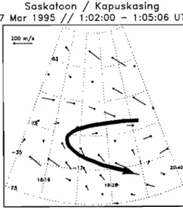
3.1. Convection Reversal
In this example, we use data from the Saska-
toon/Kapuskasing radar pair, measured in the dusk
sector on March 7, 1995, between 0102 and 0105 UT. Figure 4 shows the convection maps obtained with
the standard merging method (Figure 4a) and the high-resolution method (Figure 4b). These two maps
show, in geomagnetic coordinates, a well-defined con- vection reversal, sketched by the superimposed bold
arrow.
In Figure 4a the convection reversal is clearly ev- ident, but the location of the velocity shear is not
well defined. This reversal seems to be character-
ized by a very smooth velocity gradient, with a typ- ical scale length of the order of 250 km. With the high-resolution method, the convection reversal ex- hibits much sharper characteristics. The velocity shear is very well localized, as shown by the dashed
line. From this map, the gradient scale length, in
Saskafoon / Kapuskasing
7 Mar 1995 // 1:02'00 - 1'05'06 UTa)
$askafoon / Kapuskasing 7 Mar 1995 // 1:02'00 - 1'05'12 UTb)
Figure 4. A convection reversal measured by the
Saskatoon/Kapuskasing radar pair as reproduced by
(a) the standard
merging
method
and (b)the high-
resolution merging method. The bold arrow sketchesthe observed convection pattern, and the dashed line
indicates the location of velocity shear.
the direction perpendicular to the shear, can be es-
timated to be about 90 km. One can note here that
the smoothing effect of the averaging process used in the standard merging method is removed by the high-resolution algorithm.
ANDR]• ET AL.' SUPERDARN HIGH-RESOLUTION MAPPING 1173
Figure 4b also illustrates the fact that all velocity vectors are not independent. Several vector groups
are identical or close to identical. This is partic-
ularly evident at high latitudes (82ømagnetic lati- tude (MLAT), between 1930 and 2030 magnetic local time (MLT)), where several vectors have the same
direction and amplitude. In this region, the MU-
SIC method was not able to extract multicomponent
spectra. This may be due to poor data quality, but it can also result from a homogeneous convection zone,
without any velocity structure.
This example shows clearly the benefits and lim-
itations of the method. It is able to define more
precisely small-scale structures and sharp variations in the convection and to quantify the structure scale
lengths. Nevertheless, it cannot solve totally the ve-
locity vector dependence problem when regular flows
are present.
Saskafoon / Kapuskasing
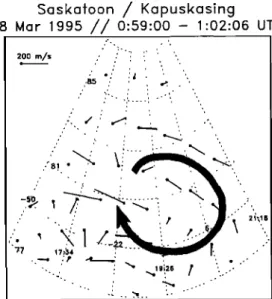
8 Mar 1995 // 0'59-00 - 1'02-06 Ua)
3.2. Vortex in the Convection
The second example was obtained on March 8,
1995, between 0059 and 0102 UT, by the Saska-
toon/Kapuskasing radar pair when a mesoscale vor-
tex is observed in the 81øMLAT and 1930 MLT sec-
tor.
Figure 5a shows the structure mapped with the standard merging method. A vortex is observed to
be embedded in an eddy flow. Despite the fact that
this vortex is not perfectly defined, we can infer a typical scale length of the order of 200 km. Fig- ure 5b shows the same vortex mapped by the high- resolution merging method. As in Figure 5b, the
vortex is embedded in an eddy flow, but the localiza-
tion of the vortex center at about 81 øand 1930 MLT
is more precise, and its typical scale size is inferred to be of the order of 100 km. Around this structure,
in the upper part of the field of view, the plasma motion is well defined and shows a large convection
reversal.
Again, the high-resolution method gives a more detailed description of the convection pattern. The typical scale size is evaluated with greater confidence, and the field-aligned currents associated with this vortex may be estimated more precisely with the
method developed by Sofko et al. [1995].
4. Discussion
The merging method developed in this paper is based on several hypotheses, which are now dis-
Saskatoon / Kapuskasing
8 Mar 1995 // 0'59:00 - 1'02:12 UT
b)
Figure 5. A vortex measured by the Saska-
toon/Kapuskasing
radar pair as reproduced
by (a)
the standard merging method and (b) the high- resolution merging method. The bold arrow sketchesthe observed convection pattern, and the cross shows
the center of the vortex.
cussed. First of all, the high-resolution spectral anal- ysis is made with the MUSIC method. Because of
its great selectivity, this method does not provide a large number of multipeaked spectra. Typically,
1174 ANDRI• ET AL.: SUPERDARN HIGH-RESOLUTION MAPPING
the probability of obtaining a double-peaked spec-
trum is at most 10% [Barthes et al., 1998], a figure which is considerably smaller than the 100% proba-
bility used in the simulation. These figures lead us to expect to reduce the mean divergence by a factor much smaller than 45%, as obtained in the simulated map. A consequence of this limited number of multi- peaked spectra is also the dependence of neighboring velocity vectors, which share a common radial ve- locity component. In the future, we may hope to reduce the dependence of the vectors by measuring more accurately the autocorrelation function or by
using a more efficient spectral analysis method. Possible localization errors are taken into account
by computing three different maps, corresponding to three different shifts applied to all radial velocities
and over the whole radar field of view. Because the estimated localization error is based on a statistical
study, we have supposed that the average ionospheric
density profile is the same for each radar beam, i.e.,
is independent of the azimuth. This strong hypoth- esis is not generally true, and we can easily suppose that a meridional beam will not experience the same ionospheric density profile as a zonal one. The iono- spheric models used in this simulation are supposed to be representative of both dayside and nightside
conditions [Andr4 et al., 1997]. We can consider that
this variability is a good estimate of the azimuthal variability of the ionospheric density profile. Then,
the fluctuation of the localization error with respect
to the ionospheric model can give an estimate of its variation with the azimuth. This error is quantified by the error bars in the Figures 2a and 2b and is of the order of 10 km, less than one range gate. Then, in a first approximation, the application of the same shift over the whole radar field of view is acceptable. Of course, a more rigorous treatment should consider
different shifts for different beams.
The computation of a velocity map leads to the
selection of several new radial velocities taken from
the multipeaked spectra and of one range offset which
corresponds to the localization adjustment. The in-
fluence of the number of new velocities determined
by MUSIC on the determination of the offset can
be questionned. Using the particular case simulated
above, the selected offset has been modified when
the proportion of multipeaked spectra did represent
at least 50% of the radar data. Thus the offset de-
termination could depend on the expected propor- tion of multipeaked spectra on a real convection map.
In most of the observed cases, this proportion never
reached more than 10% [Barthes et al., 1998]. Thus
one can expect that this value always remains below
50%, and one concludes that the presence of multi-
peaked spectra should not influence the determina- tion of the range offset.
At last, we have supposed that all the velocities measured in one range cell represent the convection velocity. This hypothesis can be wrong if the ve- locity field is made of small-scale structures super-
posed on a larger-scale convection, as hypothesized by Schiffier et al. [1997] with a specific model of
vortices. The problem can be serious if, in addition,
the scattering cross section is larger in the small-
scale structures than in the large-scale convection. If the measured radial velocity components are all
polluted by the small-scale structure, it is clear that the resulting velocity map will no longer represent
the large-scale convection, but that it will include a degree of spatial aliasing. However, we may also ex- pect an increase in the divergence in that case. On the contrary, if at least one of the measured velocity represents the convection, we may expect that it will lead to a smaller divergence.
5. Conclusions
We have presented a method which optimizes the spatial resolution of the velocity maps deduced from SuperDARN data and extracts more information on
small-scale structures (L m 200 km) present in the
ionospheric convection. We first have defined the high-resolution grid on which the velocity vectors are computed and have pointed out the difficulties in- herent in this grid. An estimate of the localization error has been given and has been shown to be of
the order of the radial resolution of the SuperDARN
radars (one grid step). The elementary cells and the
grid used imply a velocity vector dependence that we have reduced by using the MUSIC high-resolution spectral analysis. In order to give reliable results, the method is very selective, and, as a result, all vectors are not totally independent. The solutions found im- ply a selection between several maps with the help of a physical criterion. The selected map minimizes the sum of the divergence magnitudes. With simulated SuperDARN data, we have illustrated the limitations of the method. We conclude that this method gives
more information than the standard one for struc-
ANDRI• ET AL.: SUPERDARN HIGH-RESOLUTION MAPPING 1175
km. Finally, we have illustrated the method with ex- perimental SuperDARN data, showing a convection reversal and a vortex. In both cases, the method ex-
tracts more detailed information on small-scale size
features.
In conclusion, when applied to SuperDARN radar
data, the high-resolution merging algorithm gives ac-
cess to small-scale structures in the ionospheric con- vection. This can be very useful for a better under-
standing of perturbations such as the ionospheric sig-
nature of flux transfer events, traveling convection vortices, or the highly structured convection which prevails during northward interplanetary magnetic field time periods.
Acknowledgments. The Kapuskasing HF radar is funded by NASA under grant NAG5-1099. The Saskatoon HF radar is funded by an NSERC Canada Collaborative Special Project grant.
References
Andre, R., J.-P. Villain, and F. Germain, Ray-tracing program, Tech. Rep. LPCE/NTS/O22.A, 42 pp.,
Lab. Phys. Chim. Environ., Cent. Nat. de la Rech. Sci., Orleans, France, 1994.
Andre, R., C. Hanuise, J.-P. Villain, and J.-C. Cerisier,
HF radars: Multifrequency study of refraction ef- fects and localization of scattering, Radio Sci., $2,
153-168, 1997.
Baker, K.B., R.A. Greenwald, A.D.M. Walker, P.F.
Bythrow, L.J. Zanetti, T.A. Potemra, D.A. Hardy, F.J. Rich, and C.L. Rino, A case study of plasma processes in the dayside cleft, J. Geophys. Res.,
91, 3130-3144, 1986.
Barthes, L., R. Andre, J.-C. Cerisier, and J.-P. Vil- lain, Separation of multiple echoes using a high- resolution spectral analysis for SuperDARN HF radars, Radio Sci., 33,1005-1017,1998.
Breit, G., and M.A. Tuve, A test of the existence of the conducting layer, Phys. Res., 28, 554, 1926. Bristow, W.A., et al., Observations of convection vor-
tices in the afternoon sector using the SuperDARN
HF radars, J. Geophys. Res., 100, 19,743-19,756, 1995.
Cerisier, J.-C. and C. Senior, Merge: A Fortran Pro- gram, 40 pp., Cent. d'Etude des Environ. Terr. et Planet., Cent. Nat. de la Rech. Sci., St-Maur,
France, 1994.
Greenwald, R.A., et al., DARN/SuperDARN: A glo-
bal view of the dynamics of the high-latitude con-
vection, Space Sci. Rev.,71, 761, 1995a.
Greenwald, R.A., W.A. Bristow, G.J. Sofko, C. Se-
nior, J.-C. Cerisier, and A. Szabo, Super Dual Au-
roral Radar Network radar imaging of the day- side high-latitude convection under northward in- terplanetary magnetic field: Toward resolving the
distorted two-cell versus multicell controversy, J.
Geophys. Res., 100, 19,661-19,674, 1995b.
Greenwald, R.A., J.M. Ruohoniemi, W.A. Bristow,
G.J. Sofko, J.-P. Villain, A. Huuskonen, S. Kokubun, and L.A. Frank, Mesoscale dayside convection vor-
tices and their relation to substorm phase, J. Geo- phys. Res., 101, 21,697-21,713, 1996.
Jones, R.M., and J.J. Stephenson, A versatile three dimensional ray tracing program for radio waves in the ionosphere, Tech. Rep. OT 75-76, 185
pp., Off. of Telecommun., U.S. Dep. of Cornruer.,
Boulder, Colo., 1975.
Lewis, R.V., M.P. Freeman, A.S. Rodger, G.D. Reeves, and D.K. Milling, The electric field response to the growth phase and expansion phase onset of a small
isolated substorm, Ann. Geophys., 15, 289-299,
1997.
Rodger, A.S., and M. Pinnock, The ionospheric re-
sponse to flux transfert events: The first few min- utes, Ann. Geophys., 15, 685-691, 1997.
Ruohoniemi, J.M., R.A. Greenwald, K.B. Baker, J.P.
Villain, C. Hanuise, and J. Kelly, Mapping high- latitude plasma convection with coherent HF radars,
J. Geophys. Res., 94, 13,463-13,477, 1989.
Schiftter, A., G. Sofko, P.T. Newell, and R.A. Green-
wald, Mapping the outer LLBL with SuperDARN double-peaked spectra, Geophys. Res. Lett., 2•,
3149-3152, 1997.
Sofko, G.J., R. Greenwald, and W. Bristow, Direct determination of large-scale magnetospheric field- aligned currents with SuperDARN, Geophys. Res.
Lett., 22, 2041-2044, 1995.
Thorolfsson, A., it Transfert de flux magn•tique in- termittents entre le vent solaire et la magnetosphere : Th•orie et mod•lisation des signatures, 54 pp., Cent. d'Etude des Environ. Terr. et Planet., Cent. Nat. de la Rech. Sci., St-Maur, France,
1996.
Villain, J.-P., R.A. Greenwald, and J.F. Vickrey, HF ray tracing at high latitudes using measured merid- ional electron density distributions, Radio Sci., 19,
359-374, 1984.
1176 ANDRI• ET AL.: SUPERDARN HIGH-RESOLUTION MAPPING
Ruohoniemi, HF radar observations of E region
plasma irregularities produced by oblique electron
streaming, d. Geophys. _Res., 9œ, 12,327-12,342, 1987.
Wei, C.Q., and L.C. Lee, Ground magnetic signa-
tures of moving elongated plasma clouds, d. Geo- phys. Res., 95, 2405-2418, 1990.
Yeoman, T.K., and H. Luhr, CUTLASS/IMAGE ob-
servations of high-latitude convection features dur-
ing substorms, Ann. Geophys., 15, 692-702, 1997.
Avenue de la Recherche Scientifique, 45071 Orleans
cedex 2, France.
L. Barthes, J. C. Cerisier, C. Senior, and A.
Thorolfsson, Centre d'Etude des Environnements Terrestres et Planetaires, CNRS, 4 Avenue de Nep-
tune, 94107 Saint-Maur-des-Foss•s Cedex, France.
C. Hanuise, Laboratoire de Sondage Electromag- n•tique de l'Environnement Terrestre, CNRS, Uni-
versit• de Toulon, BP 132, 83957 La Garde, France
R. Andr• and J. P. Villain, Laborat&re de
Physique et Chimie de l'Environnement, CNRS, 3A
(Received August 4, 1998; revised January 25, 1999; accepted April 7, 1999.)