HAL Id: hal-02311475
https://hal-amu.archives-ouvertes.fr/hal-02311475v2
Submitted on 11 Oct 2019
HAL is a multi-disciplinary open access
archive for the deposit and dissemination of
sci-entific research documents, whether they are
pub-lished or not. The documents may come from
teaching and research institutions in France or
abroad, or from public or private research centers.
L’archive ouverte pluridisciplinaire HAL, est
destinée au dépôt et à la diffusion de documents
scientifiques de niveau recherche, publiés ou non,
émanant des établissements d’enseignement et de
recherche français ou étrangers, des laboratoires
publics ou privés.
Adaptive Estimation of the Thermal Behavior of
CPU-GPU SoCs for Prediction and Diagnosis
Oussama Djedidi, Nacer K M’Sirdi, Aziz Naamane
To cite this version:
Oussama Djedidi, Nacer K M’Sirdi, Aziz Naamane. Adaptive Estimation of the Thermal Behavior
of CPU-GPU SoCs for Prediction and Diagnosis. Proceedings of the International Conference on
Integrated Modeling and Analysis in Applied Control and Automation, 2019–IMAACA 2019, Sep
2019, Lisbon, Portugal. pp.93-98. �hal-02311475v2�
ADAPTIVE ESTIMATION OF THE THERMAL BEHAVIOR OF CPU-GPU SOCS FOR
PREDICTION AND DIAGNOSIS
Oussama Djedidi(a), Nacer K. M’Sirdi(b), Aziz Naamane(c)
(a),(b),(c) Aix Marseille University, Université de Toulon, CNRS, LIS UMR 7020, SASV, Marseille, France (a)[email protected], (b)[email protected], (c)[email protected]
ABSTRACT
This paper proposes a dynamic behavioral model for temperature variations of systems on chips (SoC) in embedded systems. We use identification techniques (ARMAX modeling) to construct a data-driven online temperature model that estimates the temperature according to the CPU and GPU frequencies, the used RAM and the power consumed by the chip. Furthermore, we used two the Recursive Least Squares (RLS) to estimate the parameters of the ARMAX model. This method allows us to update the parameters of the model online in case of a change in the system or its characteristics. Finally, we validate the temperature model and compare between booth estimation methods. Keywords: Identification, Embedded systems, Control
1. INTRODUCTION
Since their introduction in 1971, microprocessors have evolved from simple calculators to the center of all technological innovations (Faggin, Hoff, Mazor, and Shima, 1996). The ubiquity of microprocessor-based systems has pushed for the study of their behavior and reliability, notably when used in safety-critical and sensitive systems. Thus, the modeling and diagnosis of the microprocessor-based systems is, now, an ongoing scientific and engineering endeavor.
These systems are evermore evolving and increasing in complexity both on the microarchitectural and process levels, giving rise to new challenges with every new generation. This paper is a part of a project that explores yet another evolution enabled by these systems; the development of avionic cockpits operated by touchscreens (Figure 1). The embedded SoC used in such a critical system is required to be failproof, which require them to be studied from all physical and software aspects. In this particular work, we focus on the thermal behavior of the SoC behind the touchscreen.
Of the many aspects of modeling systems-on-chips (SoC), the temperature is one of the few that links the software, mechatronic and physical characteristics. Hence, many of the recent work studying it were studied on the thermal effects on system radiality (Löfwenmark and Nadjm-Tehrani, 2018), its management for a better reliability (Niu and Zhu, 2017, Zhou et al., 2018) or better scheduling and power management (Li, Yu, and
Song, 2018). Our work, however, is oriented towards the real-time surveillance of the chip (Djedidi, Djeziri, and M’Sirdi, 2018). It concentrates on the monitoring of the chip to detect the presence of any anomalies of abnormal behavior.
Figure 1: A prototype of the cockpit of the future by Thales Avionics (Thales, 2017).
In the next section, we further detail the goal of our and put into the context of our previous works. In section 3, we discuss the thermal modeling of CPU-GPU, then we present and apply identification-based modeling to model the thermal devious of the SoC in section 4. Finally, the results and concluding remarks are presented in sections 5 and 6.
2. THE STUDIED SYSTEM
The objective of this work is the mechatronic modeling of the CPU-GPU SoC in embedded systems to predict their behavior. This behavior prediction can then be used for monitoring and diagnosis. This work is also a continuation of the works by Djedidi et al. (2017) and Djedidi, Djeziri, and M’Sirdi (2018), where the authors worked on the modeling and monitoring of systems designed for safety-critical environments. In the first study, Djedidi et al. (2017) developed an incremental interconnected modeling approach, to estimate key variables that determine the operating state of the system (Frequencies and voltages of the CPU, and GPU, Memory Occupation Rate (MOR), Chip Temperature and power consumption). Figure 2 shows a generalized diagram of the established model for mobile CPU-GPU SoC with 𝑛 CPU cores.
Figure 2: Synoptic diagram of the incremental interconnected model for a CPU-GPU SoC (Djedidi et al., 2017).
The developed model was then used to monitor the state the SoC and for the online detection of several types of faults such as software bugs and environmental faults (Djedidi et al., 2018).
This work focuses on temperature modeling and estimation. It aims to build a model that can be used to predict the temperature values of the SoC according to the current workload. The model is also to be integrated in the interconnected modelling framework as the thermal model (Figure 2). Finally, it is also intended to be used for the diagnosis of the chip in the future.
The case study we used to validate, and test model is a safety-critical certified development board ( Figure 3). The board runs on Linux and is Android capable. It has a one core ARM Cortex-A9 processor and is equipped with 1 Gb of RAM (Freescale Semiconductor Inc, 2012b).
Figure 3: View of the test installation with the development board in the middle connected to the monitoring PC.
3. THERMAL MODELING
To model the thermal behavior of an embedded system, the first step is to follow the heat flow.
Figure 4: Simplified cross section of a typical SoC with a die containing the CPU, GPU and RAM, installed on a PCB.
Figure 4 shows, how in the SoC, heat is generated by the circuitry containing the processor cores and the RAM. It is then transferred through conduction in two directions to the silicon case (top), the underfill and the C4 bumps (bottom). The latter two would then conduct the heat to the substrate which itself would conduct it to the printed circuit board (PCB). Finally, the heat is dissipated by the case and the PCB to the air through convection and
radiation. In these circuits, heat transfer occurs mostly from one layer to another (vertically, in the diagram).
Figure 5: Equivalent thermal resistance circuit of a typical integrated circuit of an SoC.
Figure 5 shows the equivalent thermal resistance circuit (Freescale Semiconductor Inc, 2012a, Wang, Sun, and Pan, 2017). The thermal resistance circuit can be used to build a model that describes the evolution of the temperature from one layer to another. The heat (𝑄) can be written as:
𝑄 = 𝑄𝐽/𝑆𝑖+ 𝑄𝐽/𝑈+ 𝑄𝐽/𝐶4+ 𝑄𝑆𝑖/𝐴𝑖𝑟+ 𝑄𝐶4/𝑆𝑢
+ 𝑄𝑈/𝑆𝑢+ 𝑄𝑆𝑢/𝑃𝐶𝐵+ 𝑄𝑃𝐶𝐵/𝐴𝑖𝑟
(1)
Where 𝑄 is equal, in each layer, to the temperature difference divided by the thermal resistance of the said layer (Wang et al., 2017). For instance, the heat transfer between the junction and the silicon encasing is equal to:
QJ/Si=
Tj− TSi
𝑅𝑆𝑖
(2)
Where 𝑅𝑆𝑖 is the thermal resistance of the silicon. Its
value can be determined either by studying the material property (area and thermal conductivity), or empirically through identification.
Models built using this method are crucial for the thermal management of the SoC. They enable engineers and system builders to correctly design the optimal cooling method (heatsink, fan, vapor chambers…). However, they also require a deep knowledge of the system and an estimation of the energy drawn by the SoC and transformed into heat which increases the complexity of the modeling process. It also does not allow for the prediction of the temperature of the SoC according to operating conditions (workload and frequency), nor the change of its value with time and degradation.
Identified models, on the other hand rely mostly on a combination of human expertise and observations to choose which inputs correlate best with the output. In this work, we use an auto-regressive model with exogenous input to predict the temperature of the SoC.
4. IDENTIFICATION-BASED MODELING
ARMAX models are polynomial models used to estimate or predict the output depending on its previous values alongside those of the input vector (Landau and Gianluca, 2006). Our choice settled on a polynomial model—precisely an ARMAX one—because they are dynamic and also fast enough to be used to generate online estimation at frequencies up to 50 Hz. Furthermore, since these models are dynamic, they can also be used to accurately simulate the behavior of the system offline and predict the operating temperature of the SoC.
A discrete ARMAX process can be described by the difference equation (Landau and Gianluca, 2006): 𝑦(𝑘) = 𝑎1𝑦(𝑘 − 1) + ⋯ + 𝑎𝑛𝑎𝑦(𝑘𝑛) + 𝑏1,1𝑢1(𝑘 − 𝜏) + ⋯ + 𝑏𝑚,𝑛𝑏𝑢𝑚(𝑘 − 𝜏 − 𝑛𝑏) + 𝑒(𝑡) + 𝑐1𝑒(𝑡 − 1) + ⋯ + 𝑐𝑛𝑐𝑒(𝑡 − 𝑛𝑐) (3)
where 𝑦(𝑘) represents the output, 𝑢(𝑘) the input vector with 𝑚 width, and 𝑒(𝑡) the error value. The parameters [𝑎1, … , 𝑎𝑛𝑎] are the regression parameters,
[𝑏1,1, … , 𝑏𝑚,𝑛𝑏] are the input parameters, and [𝑐1, … , 𝑐𝑛𝑐]
are the moving average parameters. Finally, 𝑛𝑎, 𝑛𝑏 and
𝑛𝑐 are the orders of the model, and 𝜏 is the input delay.
In our case study, the output to be estimated is the temperature 𝑇 of the SoC, and the inputs are the frequencies of the cores and the memory occupation rate (MOR). These inputs are the variables that correlate the most with the temperature (Mercati, Paterna, Bartolini, Benini, and Rosing, 2017, Niu and Zhu, 2017, Zhou et al., 2018).
+
𝜀𝑘= 𝑦𝑘 − 𝑦̂𝑘 (4)
𝑦̂(𝑘) is the predicted output. We rewrite equation (3) as a discrete linear model:
𝐴(𝑞−1)𝑦(𝑘) = 𝐵(𝑞−1)𝑢(𝑘 − 𝜏) + 𝐶(𝑞−1)𝑒(𝑘) (5)
with 𝑞−1 being the delay operator, and 𝐴(𝑞−1) = 1 +
∑𝑛𝑖=1𝑎 𝑎𝑖𝑞−𝑖, 𝐵(𝑞−1) = 1 + ∑ 𝑏𝑗,𝑖 𝑛𝑏
𝑖=1 𝑞−𝑖, and 𝐶 = 1 +
∑ 𝑐𝑗,𝑖 𝑛𝑐
𝑖=1 𝑞−𝑖. Thus, predicted output at the sample 𝑘
becomes: 𝑦̂(𝑘) =𝐵(𝑞 −1) 𝐴(𝑞−1) 𝑢(𝑘 − 𝜏) + 𝐶(𝑞−1) 𝐴(𝑞−1)𝑒(𝑘) (6)
Based upon this, we construct an adaptive predictor. This latter follows the model described in equation (6):
𝑦̂𝑘= 𝜃̂𝜑𝑘−1 (7)
with 𝑦̂𝑘 being the vector of the temperature value,
𝜑𝑘−1= [𝑦(𝑘 − 1), … , 𝑦(𝑘 − 𝑛𝑎), 𝑢1(𝑘 −
𝜏), … , 𝑢𝑚(𝑘 − 𝜏 − 𝑛𝑏), 𝜀(𝑘 − 1), … , 𝜀(𝑘 − 𝑛𝑐)] being a
vector composed of the output feedback, the inputs, and the prediction error, and 𝜃̂ = [−𝑎1, … , 𝑐𝑛𝑐] being the
vector the parameters vector.
The listing presented in Algorithm 1 is a pseudo-code describing how the parameters of the ARMAX model will be calculated with each iteration for a whole test vector 𝑦(𝑘) (Landau, M’Sirdi, and M’Saad, 1986). Algorithm 1: Pseudo-code for the recursive Least square algorithm.
1: Begin
2: Define orders: 𝑛𝑎, 𝑛𝑏, 𝑛𝑐
3: Define the input delay: 𝜏
4: // Initialization of 𝜑𝑘−1 5: Initialize 𝜑𝑦𝑘−1 6: Initialize 𝜑𝑢𝑘−𝜏 7: Initialize 𝜑𝜀𝑘−1 8: 𝜑𝑘−1← [𝜑𝑦𝑘−1, 𝜑𝑢𝑘−𝜏, 𝜑𝜀𝑘−1 ] 9: 𝜃̂𝑘−1← zeros(𝜑𝑦𝑘−1.length, 1)
10: // Initialization of an empty vector
11: 𝐹 ← 100 × eye(𝜑𝑦𝑘−1.length)
12: 𝑦(𝑘) ←Read(Output) 13: While 𝑦(𝑘) ≠ null do 14: 𝑦̂(𝑘) ← 𝜃̂𝑘−1𝜑𝑘−1
15: 𝜀(𝑘) = 𝑦(𝑘) − 𝑦̂(𝑘)
16: // Recalculation of the parameters vector
17: 𝐺 ← 𝐹 ∙ 𝜑𝑘−1 18: norm ← 1 + 𝜑𝑘−1∙ 𝐺 19: 𝐹 ← 𝐹 −𝐺∙𝐺𝑇 norm 20: 𝜃̂𝑘−1← 𝜃̂𝑘−1+ 𝐺 ∙ 𝜀(𝑘) 21: // Updating𝜑𝑘−1 22: 𝜑𝑦𝑘−1.addFirst(−𝑦(𝑘)) 23: 𝜑𝑦𝑘−1.poll(𝑛𝑎+ 1) 24: 𝜑𝑢𝑘−𝜏.addFirst(Read(Input(1:m))) 25: 𝜑𝑢𝑘−𝜏.poll(𝑛𝑏+ 1: 𝑛𝑏+ 1 + 𝑚) 26: 𝜑𝜀𝑘−1.addFirst(𝜀(𝑘)) 27: 𝜑𝜀𝑘−1.poll(𝑛𝑐+ 1) 28: 𝜑𝑘−1← [𝜑𝑦𝑘−1, 𝜑𝑢𝑘−𝜏, 𝜑𝜀𝑘−1 ]
29: \\ Reading the next output
30: 𝑦(𝑘) ←Read(Output)
31: End
5. RESULTS AND DISCUSSION
The results presented in this section are established during controlled experiments. The experiment starts when the data acquisition starts. It begins with two standards benchmarks: AnTuTu (AnTuTu, 2019) and 3DMark (Futuremark Oy, 2019), then goes on to playing and interacting with a Sudoku game, followed by 4 minutes of web browsing, HD video playback, and 4 minutes of standby time.
During this scenario, data is gathered and sent to the monitoring PC where the ARMAXRLS model is trained at
the same time with a predefined set of orders. Once the best set of orders is found, multiple trials are again launched with a different number of training samples each time. Once the training is finished, the accuracy of the model is then validated online.
Finally, to compare the methodologies, a similar ARMAX model is trained offline with the traditional
least squares method (ARMAXLS) using the same data as
the equivalent ARMAXRLS. The model is then validated,
again, with same data used to validate the equivalent ARMAXRLS model.
The results presented for the accuracy of the model are the results obtained from validation trials and sets containing about 11 × 104 samples (about 3000 s).
5.1. Order selection
The first set of trials was launched with different sets of orders. The best set is chosen according to two criteria; the Mean Absolute Percentage Error (MAPE) and the average time required to generate estimations by the model.
While higher estimation accuracy is a virtue, models with higher orders may require longer times to generate estimations which can lead to missing the changes of variables values. The time required to generate estimation is also heavily affected by OS scheduling and interruptions on both the device and the monitoring PC. Thus, the optimal model needs to satisfy both accuracy and speed of estimation constraints.
Table 1: Evolution of the accuracy and the time needed to generated estimation of the ARMAXRLS model
according to its orders. Orders of the model MAPE (%) Average Sampling Time (s) 𝑛𝑎 𝑛𝑏 𝑛𝑐 2 2 2 11.1853 18 ×10-3 3 3 3 7.9672 18 ×10-3 4 4 4 1.3757 ~30 ×10-3 4 4 2 0.8377 ~25 ×10-3 5 5 2 0.7215 ~65 ×10-3 6 6 2 1.3667 ~135 ×10-3
Table 1 displays the MAPE and the average sampling time for several sets of model orders [𝑛𝑎, 𝑛𝑏, 𝑛𝑐]. The
data in the tables show that the accuracy of the model increases with the increase of the orders up until [4,4,4], where a lower order for the moving average actually results in an increase in accuracy. Furthermore, Table 1 also show how the average sampling time increases with the order of the model, until it even starts affecting the accuracy of the model due to the longer wait time for estimations. Hence, from these experimental data, the best model orders according to both the accuracy and sampling time are [4,4,2].
5.2. Number of samples
In theory, the ideal training set would contain data representing all possible information about the system. However, in practice, the information in the training set is limited by the sample number and information contained in that sample. Table 2 shows how the accuracy of the model increases with the number of samples. However, it also shows that this increase in the accuracy is not absolute, and the accuracy might decrease even with increase number of samples. This is also shown in the comparisons shown in Figure 6 and Figure 7. Hence, the solution to obtain the best model (In this
case, 𝑛 = 3000) is to by comparison of the Mean Squared Error (MSE) as shown in Algorithm 2. Algorithm 2: Pseudo-code the selection of the best model.
1: Begin
2: 𝑀𝑆𝐸𝑐𝑢𝑟𝑟𝑒𝑛𝑡= ∑𝑛𝑖=1(𝑦𝑖−𝑦̂𝑖) 2
𝑛
3: // 𝑛 is the number of samples
4: If (𝑀𝑆𝐸𝐶𝑢𝑟𝑟𝑒𝑛𝑡< 𝑀𝑆𝐸𝑏𝑒𝑠𝑡) then
5: 𝑀𝑆𝐸𝑏𝑒𝑠𝑡← 𝑀𝑆𝐸𝐶𝑢𝑟𝑟𝑒𝑛𝑡
6: 𝑀𝑜𝑑𝑒𝑙𝑏𝑒𝑠𝑡← 𝑀𝑜𝑑𝑒𝑙𝑐𝑢𝑟𝑟𝑒𝑛𝑡
7: End
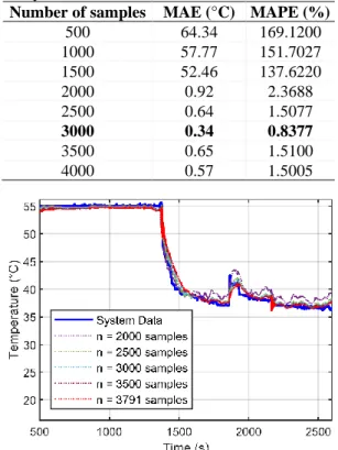
Table 2: The influence of the number of samples on the accuracy of the model.
Number of samples MAE (°C) MAPE (%)
500 64.34 169.1200 1000 57.77 151.7027 1500 52.46 137.6220 2000 0.92 2.3688 2500 0.64 1.5077 3000 0.34 0.8377 3500 0.65 1.5100 4000 0.57 1.5005
Figure 6: Estimations generated by multiple ARMAXRLS
models with different sample numbers in their training sets against system measurements.
Figure 7: Estimation error (after model convergence) of the ARMAXRLS according to the number of samples (𝑛)
5.3. Comparison with ARMAXLS
Most of the ARMAX models are trained using least-squares method. Using the same data with which the ARMAXRLS model was trained, a new ARMAXLS was
also trained with [4,4,2] as a set of orders. The model was then tested and validated using the same test data used to validate ARMAXRLS one. Table 3 show a comparison of
the MAE of the ARMAXRLS and ARMAXLS models.
While the ARMAXLS shows a slight advantage in its
offline validation results, online estimation—our case use— demonstrates an advantage for the ARMAXRLS. A
further comparison of the estimations and estimation errors are shown in Figure 8 and Figure 9.
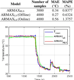
Table 3: The MAE and MAPE validation results for the ARMAXRLS and ARMAXLS models.
Model Number of samples MAE (°C) MAPE (%) ARMAXRLS 3000 0.34 0.8377 ARMAXLS (Offline) 4000 0.27 0.6324 ARMAXLS (Online) 4000 0.56 1.3757
Figure 8: Estimations generated by the ARMAXRLS and
the ARMAXLS models against system measurements.
Figure 9: Estimation error (after model convergence) of the ARMAXRLS and the ARMAXLS models.
All the results mentioned above clearly validate the ARMAXRLS. However, the high accuracy of the model
(being 99.1623%), along with its speed of estimations are not the only advantages of this model. One last advantage is the capacity to retrain the model at will without
stopping the monitoring process this can prove useful when a change in operating condition or a drop in the accuracy occur.
6. CONCLUSION
In this paper, we have built and validated ARMAX model to predict the temperature of embedded SoCs according to the workload and operating conditions. The model is trained using RLS method which offer two clear advantages over the traditional LS method. These advantages are a better online accuracy, and the capacity of training and retraining the model online without having to stop the monitoring process.
The model offers high accuracy with a mean absolute error of only 0.34°C, and also satisfy the required sampling time.
Having validated the model with satisfactory results, it will now integrated in the interconnected incremental framework we previously developed (Djedidi et al., 2018, 2017). In future works, we will be studying the effects of the temperature on the reliability of the system, and plan on using the ARMAXRLS model in the diagnosis
of the state of health of the SoC.
REFERENCES
AnTuTu. , 2019. AnTuTu Benchmark - Android Apps on
Google Play Retrieved from
https://play.google.com/store/apps/details?id=com .antutu.ABenchMark.
Djedidi, O., Djeziri, M. A., and M’Sirdi, N. K. , 2018. Data-Driven Approach for Feature Drift Detection in Embedded Electronic Devices. IFAC-PapersOnLine, 51(24), 1024–1029.
Djedidi, O., Djeziri, M. A., M’Sirdi, N. K., and Naamane, A. , 2017. Modular Modelling of an Embedded Mobile CPU-GPU Chip for Feature Estimation. In Proceedings of the 14th International Conference on Informatics in Control, Automation and Robotics (Vol. 1, pp. 338–345). Mardrid, Spain: SciTePress.
Faggin, F., Hoff, M. E., Mazor, S., and Shima, M. , 1996. History of the 4004. IEEE Micro, 16(6), 10–20. Freescale Semiconductor Inc. , 2012a. i.MX 6 Series
Thermal Management Guidelines.
Freescale Semiconductor Inc. , 2012b. i.MX 6SoloX Automotive and Infotainment Applications Processors - Data Sheet. Freescale Semiconductor. Benchmark - Android Apps on Google Play Retrieved
from
https://play.google.com/store/apps/details?id=com .futuremark.dmandroid.application.
Landau, I. D., and Gianluca, Z. (Eds.). , 2006. System Identification: The Bases BT - Digital Control Systems: Design, Identification and Implementation (pp. 201–245). London: Springer London.
Landau, I. D., M’Sirdi, N., and M’Saad, M. , 1986. Techniques de modélisation récursive pour
l’analyse spectrale paramétrique adaptative. Revue de Traitement Du Signal, 3, 183–204.
Li, T., Yu, G., and Song, J. , 2018. Minimizing energy by thermal-aware task assignment and speed scaling in heterogeneous MPSoC systems. Journal of Systems Architecture, 89, 118–130.
Löfwenmark, A., and Nadjm-Tehrani, S. , 2018. Fault and timing analysis in critical multi-core systems: A survey with an avionics perspective. Journal of Systems Architecture, 87, 1–11.
Mercati, P., Paterna, F., Bartolini, A., Benini, L., and Rosing, T. Š. , 2017. WARM: Workload-Aware Reliability Management in Linux/Android. IEEE Transactions on Computer-Aided Design of Integrated Circuits and Systems, 36(9), 1557– 1570.
Niu, L., and Zhu, D. , 2017. Reliability-aware scheduling for reducing system-wide energy consumption for weakly hard real-time systems. Journal of Systems Architecture, 78, 30–54.
Thales. , 2017. What is new on Avionics 2020? | Thales Aerospace BlogThales Aerospace Blog Retrieved from http://onboard.thalesgroup.com/new-avionics-2020/.
Wang, K. J., Sun, H. C., and Pan, Z. L. , 2017. An analytical thermal model for Three-Dimensional integrated Circuits with integrated micro-channel cooling. Thermal Science, 21(4), 1601–1606. Zhou, J., Yan, J., Cao, K., Tan, Y., Wei, T., Chen, M., …
Hu, S. , 2018. Thermal-aware correlated two-level scheduling of real-time tasks with reduced processor energy on heterogeneous MPSoCs. Journal of Systems Architecture, 82, 1–11.