HAL Id: hal-00021237
https://hal.archives-ouvertes.fr/hal-00021237
Submitted on 21 Mar 2006
HAL is a multi-disciplinary open access
archive for the deposit and dissemination of sci-entific research documents, whether they are pub-lished or not. The documents may come from teaching and research institutions in France or
L’archive ouverte pluridisciplinaire HAL, est destinée au dépôt et à la diffusion de documents scientifiques de niveau recherche, publiés ou non, émanant des établissements d’enseignement et de recherche français ou étrangers, des laboratoires
Condensation in a Disordered Infinite-Range Hopping
Bose–Hubbard Model
T. C. Dorlas, L. A. Pastur, V. A. Zagrebnov
To cite this version:
T. C. Dorlas, L. A. Pastur, V. A. Zagrebnov. Condensation in a Disordered Infinite-Range Hopping Bose–Hubbard Model. Journal of Statistical Physics, Springer Verlag, 2006, 124 (5), pp.1137-1178. �10.1007/s10955-006-9176-x�. �hal-00021237�
Condensation in a Disordered Infinite-Range
Hopping Bose-Hubbard Model
T.C.DORLAS1, L.A.PASTUR2 and V.A. ZAGREBNOV3
Dublin Institute for Advanced Studies, School of Theoretical Physics, 10 Burlington Road, Dublin 4, Ireland1
Department of Theoretical Physics of Institute for Low Temperature Physics and Engineering
47 Lenin Avenue, Kharkov 310164, Ukraine 2
Universit´e de la M´editerran´ee and Centre de Physique Th´eorique, Luminy-Case 907, 13288 Marseille, Cedex 09, France3
Abstract
We study Einstein Condensation (BEC) in the Infinite-Range Hopping Bose-Hubbard model for repulsive on-site particle interaction in presence of ergodic random one-site potentials with different distributions. We show that the model is exactly soluble even if the on-site interaction is random. But in contrast to the non-random case [BD], we observe here new phenomena: instead of enhancement of BEC for perfect bosons, for constant on-site repulsion and discrete distributions of the single-site potential there is suppression of BEC at some fractional densities. We show that this suppression appears with increasing disorder. On the other hand, the BEC suppression at integer densities may disappear, if disorder increases. For a continuous distribution we prove that the BEC critical temperature decreases for small on-site repulsion while the BEC is suppressed at integer values of density for large repulsion. Again, the threshold for this repulsion gets higher, when disorder increases.
1
DIAS-School of Theoretical Physics - email: [email protected]
2
Department of Theoretical Physics of ILTPE - email: [email protected]
3
1
Introduction
Lattice Bose-gas models were invented as an alternative way to understand continuous inter-acting boson systems including liquid Helium, see [MM] and a very complete review [U]. But recent experiments with cold bosons in traps of three-dimensional optical lattice potentials show that lattice models are also relevant for describing the experimentally observed Mott insulator -superfluid (or condensate) phase transition [G-B]. In [BD] and then in [A-Y], this phenomenon was analyzed rigorously in the framework of the so-called Bose-Hubbard model.
The aim of the present paper is to study a disordered Bose-Hubbard model and in particular the influence of the single-site potential randomness on the Bose-Einstein condensate (BEC).
Notice that the first attempts to understand this influence go back to [KL1], [KL2] and [LS] for continuous Perfect Bose-Gases (PBG) in a random potential of impurities. For the rigorous solution of this problem see [L-Z]. One of the principal result of [L-Z] is that the randomness enhances the BEC. For example, the one-dimensional PBG has no BEC because of the high value of the one-particle density of states in the vicinity of the bottom of the spectrum above the ground state, making the integral for the critical particle density infinite. The presence of a non-negative homogeneous ergodic random potential modifies the one-particle density of states (due to the Lifshitz tail ) in such a way that the integral for the critical density becomes finite. Hence, the one-dimensional PBG with random potential does manifest BEC. The nature of this BEC is close to what is known as the ”Bose-glass” since it may be localized by the random potential [LZ]. This is of interest for experiments with liquid 4He in random environments like
Aerogel and Vycor glass, [F-F], [KT].
On the other hand, the nature and behaviour of the lattice BEC may be quite different. First of all, the lattice Laplacian and the Bose-Hubbard interaction produce a coexistence of the BEC (superfluidity) and the Mott insulating phase as well as domains of incompressibility, see e.g. [F-F], [K-C]. Adding disorder makes the corresponding models much more compli-cated. The physical arguments [F-F], [K-C] show that the randomness may suppress the BEC (superfluidity) as well as the Mott phase in favour of the localized Bose-glass phase, but this is very sensitive to the choice of the random distribution.
Since there are very few rigorous results about the BEC in disordered systems, we consider here a single-site random version of the lattice Infinite-Range Hopping (IRH) Bose-Hubbard model, which in non-random case has recently been studied in detail for all temperatures and chemical potentials in [BD].
This paper is organized as follows. In Section 2, we define the lattice Laplacian for finite-and infinite-range hopping finite-and recall the results about BEC for the free lattice Bose-gas. We then introduce random single-site and on-set particle interaction potentials and state our main result about the existence of and an explicit formula for the pressure for the IRH Bose-Hubbard model with these type of randomness. We outline the proof of the main theorem using the approximating Hamiltonian method.
In Section 3 we consider the pressure for extremal cases of hard-core and perfect bosons. We show that they are the limits of the IRH Bose-Hubbard model pressure when the on-site particle interaction tends respectively to +∞ and to 0.
In Section 4, we analyse the phase diagram in the case of a non-random on-site particle interaction and random single-site external potential. We distinguish a number of different cases. We start with perfect bosons and show that the randomness enhances BEC in this case, see Sect.4.1. This is no longer true for interacting bosons. We study in Sect.4.2 the phase diagram first for Bernoulli single-site potential and then for trinomial and multinomial discrete
distributions.
In the case of a Bernoulli distribution and hard-core bosons (infinite on-set repulsion) we showe that in addition to the complete BEC suppression at extremal allowed densities ρ = 0 and ρ = 1 there is a new point ρ = 1−p, where p = Pr {potential 6= 0}. We prove that for finite on-site repulsion the suppression of BEC at integer, and also for fractional values of densities ρ = n− p , n = 1, 2, . . . persists, if the Bernoulli potential amplitude is large enough. In fact we find that increasing the Bernoulli potential amplitude (disorder) decreases the critical BEC temperature in the vicinity of fractional values of densities but increases it for integer values of density. A similar phenomenon occurs also for equiprobable trinomial distributions, but now for densities ρ = n/3. Our numerical calculations demonstrate that it should be true for a general multinomial distribution.
For illustration of a continuous distribution we study a homogenous distribution with com-pact support. Then for hard-core bosons we prove that the complete BEC suppression occurs only at extremal allowed densities ρ = 0 and ρ = 1, with the trace of suppressions only at integer values of densities for a finite on-site repulsion. In particular we show that the critical BEC temperature gets lower, when one switches on disorder for (a small) on-site interaction, whereas it gets higher for perfect bosons. For large values of on-site interaction the picture is similar to the discrete distributions: increasing of disorder increases the critical BEC temper-ature in the vicinity of integer values of density but increases it for the complimentary values of density.
In Section 5 we summarize and discuss our results.
2
Model and Main Theorem
For simplicity we shall consider the Bose-Hubbard model only with periodic boundary condi-tions. So let Λ := {x ∈ Zd : −L
α/2 ≤ xα < Lα/2, α = 1, . . . , d} be a bounded rectangular
domain of the cubic lattice Zd wrapped onto a torus. Then the set Λ∗ := {q
α = 2πn/Lα :
n = 0,±1, ±2, . . . ± (Lα/2− 1), Lα/2, α = 1, 2, . . . d} is dual to Λ with respect to Fourier
transformation on the domain Λ = L1× L2× . . . × Ld of volume |Λ| = V .
The standard one-particle Hilbert space for the set Λ can be taken as h(Λ) := CΛ with the
canonical basis {ex}x∈Λ, i.e. ex(y) = δx , y. Then for any element u = Px∈Λuxex ∈ h(Λ) the
one-particle kinetic-energy (hopping) operator is defined by (tΛu)(x) := X y∈Λ tΛx , y(u(x)− u(y)) = X y∈Λ tΛx , y(ux− uy), (2.1) where tΛx y= 1 V X q∈Λ∗ ˆ tqeiq(x−y) , (2.2)
is the periodic extension in domain Λ of a symmetric, translation invariant and positive-definite matrix, i.e. ˆ tq= X y∈Λ tΛ0 , yeiqy ≥ 0. (2.3)
Notice that functions {(ˆeq)(y) := eiqy/
√
V}q∈Λ∗ also form a basis in h(Λ), i.e. for any u∈ h(Λ)
one has u = P
Let FB := FB(h(Λ)) be the boson Fock space over h(Λ). For any f ∈ h(Λ)) we can associate
in this space the creation and annihilation operators a∗(f ) :=X
y∈Λ
a∗(y)f (y) , a(f ) :=X
y∈Λ
a(y)f∗(y) . (2.4)
Let a∗
x, ax and ˆa∗q, ˆaq be the boson creation and annihilation operators corresponding
respec-tively to the basis elements ex and ˆeq, satisfying the lattice Canonical Commutation Relations:
£ax, a∗y¤ = δx , y and £ˆaq, ˆa∗p¤ = δq , p. Then nx = a∗xax is the one-site number operator, and
NΛ:= X x∈Λ nx = X q∈Λ∗ ˆ a∗qˆaq, (2.5)
is the total number operator.
The second quantization of the hopping operator (2.1) in FB gives the free boson Hamilton
of the form TΛ:= X x ∈Λ a∗x(tΛa)x = 1 2 X x,y ∈Λ tΛx y(a∗x− a∗y)(ax− ay) = X q∈Λ∗ (ˆt0− ˆtq)ˆa∗qˆaq. (2.6)
If hopping is allowed only between the nearest neighbor (n.n.) sites with equal probabilities, then tΛ=−∆ corresponds to minus the lattice Laplacian, i.e.
tΛx y= d
X
α=1
(δx+1α, y+ δx−1α, y), (2.7)
where (x± 1α)β = xβ± δα , β. In this case the one-particle hopping operator spectrum is
ǫ(q) := (ˆt0− ˆtq) = d
X
α=1
4 sin2(qα/2) ≥ 0 , q ∈ Λ∗ , (2.8)
with eigenfunctions {ˆeq}q∈Λ∗.
It is known that the lattice free Bose-gas (2.6) with n.n. hopping manifests the zero-mode BEC when d > 2, since the spectral density of states Nd(dǫ) corresponding to (2.7) is small
enough to make the critical particle density ρf ree
c (β) bounded for a given temperature β−1 :
ρf reec, n.n.(β) := lim µ↑0limΛ 1 V X q∈Λ∗ 1 eβ(ǫ(q)−µ)− 1 = 1 (2π)d Z Bd ddq 1 eβǫ(q)− 1 (2.9) = Z R+ Nd(dǫ) 1 eβǫ− 1 <∞ .
Here limΛ stands for the thermodynamic limit Λ ↑ Zd, by Bd := [−π, π]d we denote the first
Brillouin zone and the density of states Nd(dǫ) ={cdǫ(d/2−1)+ o(ǫ(d/2−1))}dǫ for small ǫ.
A similar result is true for the infinite-range (i.r.) hopping Laplacian: tΛx y = 1
V (1− δx , y) , x, y∈ Λ. (2.10)
By (2.10) the one-particle spectrum in this case takes the form:
Therefore, it has a gap:
lim
q→0ǫ(q) = 16= ǫ(0) = 0 , (2.12)
and allowed values of the chemical potential are still µ≤ 0. Since the density of states is simply zero in the gap, and |Λ∗| = V |Bd|, we have N
d(dǫ) = δ(ǫ− 1)dǫ. Therefore, the critical particle
density has a bounded value:
ρf reec, i.r.(β) = 1 (2π)d Z Bd ddq 1 eβ − 1 = 1 eβ − 1 <∞ , (2.13)
for any dimensions. The latter implies a zero-mode BEC for densities ρ > ρf reec, i.r.(β).
The problem of existence of BEC gets much less obvious if one takes into account the boson interaction. This is even the case for the simplest on-site repulsive interaction
HΛ := TΛ+ λ
X
x∈Λ
nx(nx− 1) , λ ≥ 0 , (2.14)
known as the Bose-Hubbard model. (Notice that attraction: λ < 0 makes this model unstable, see [U] for discussion of other cases.)
Remark 2.1 Concerning the model (2.14) the best rigorous results so far are:
- a proof of BEC for the n.n. lattice Laplacian and the hard-core boson repulsion: λ = +∞, by [K-S] for the case of the half-filled lattice, see also [AB];
- a recent exact solution of the IRH Bose-Hubbard model (2.10), (2.14) for any λ ≥ 0 by [BD]. The aim of the the present paper is to study a disordered IRH Bose-Hubbard model. Let (Ω, Σ, P) be a probability space. We define our basic model by the random Hamiltonian:
HΛω = 1 2V X x,y∈Λ (a∗x− a∗y)(ax− ay) + X x∈Λ λωxnx(nx− 1) + X x∈Λ εωxnx, (2.15) where parameters {λω
x ≥ 0}x∈Zd and {εωx ∈ R1}x∈Zd, for ω ∈ Ω, are real-valued random fields
on Zd, which we suppose to be stationary and ergodic. We denote by
pω Λ(β, µ) := p [HΛω] (β, µ) := 1 βV TrFBexp{−β(H ω Λ − µNΛ)} (2.16)
the grand canonical pressure of the system (2.15) for given temperature β−1 and chemical
potential µ. For non-random parameters λω
x = λ ≥ 0 and εωx = ε = 0 the model (2.15) was
considered in [BD].
Our main theorem is a formula for the pressure of this model given some general regularity conditions on the random parameters involved in the Hamiltonian (2.15).
Theorem 2.1 Let the stationary, ergodic random fields {λω
x}x∈Zd and {εωx}x∈Zd be such that:
λmin := inf x,ωλ ω x > 0 , εmin := inf x,ωε ω x >−∞. (2.17)
Then for almost all ω ∈ Ω, i.e., almost sure (a.s.), there exists a non-random thermodynamic limit of the pressure (2.16):
a.s.− lim
Λ p ω
such that p(β, µ) = (2.19) sup r≥0©−r 2+ β−1E©ln Tr (FB)xexp β [(µ− ε ω x − 1)nx− λωxnx(nx− 1) + r(a∗x+ ax)]ªª ,
where E (·) is expectation with respect to the measure P. Proof : Let H0Λω :=X x∈Λ λωxnx(nx− 1) + X x∈Λ (εωx + 1)nx . (2.20)
Then by definitions (2.4) the Hamiltonian (2.15) takes the form HΛω = TΛ+ X x∈Λ λωxnx(nx− 1) + X x∈Λ εωxnx =−ˆa0∗ˆa0+ H0Λω . (2.21)
Since conditions (2.17) imply the estimate from below: HΛω ≥ −ˆa∗0ˆa0+ NΛ+ λmin X x∈Λ nx(nx− 1) + εminNΛ (2.22) ≥ λmin V N 2 Λ+ (εmin− λmin)NΛ ,
the Hamiltonian (2.21) is superstable. Thus, the pressure in (2.18) is defined for all µ ∈ R1.
Following [B-T], we introduce a similar Hamiltonian with sources: HΛω(ν) := HΛω−
√
V (νˆa0+ νˆa∗0) , ν ∈ C , (2.23)
and the corresponding approximating Hamiltonian:
HΛω(z, ν) := H0Λω (z)−√V (νˆa0+ νˆa∗0) , (2.24) where H0Λω (z) := H0Λω + V |z| 2 −√V (zˆa0+ zˆa∗0) , z ∈ C. (2.25) Then HΛω(ν)− HΛω(z, ν) =−(ˆa0− z √ V )∗(ˆa0− z √ V ), (2.26)
and by virtue of the Bogoliubov convexity inequality one gets the estimates: 0≤ p [HΛω(ν)]− p [HΛω(z, ν)]≤ 1 V D (ˆa0− z √ V )∗(ˆa0− z √ V )E Hω Λ(ν) (2.27) for each realization ω ∈ Ω. Here h−iHω
Λ(ν) := h−iHΛω(ν)(β, µ) denotes the grand-canonical
quantum Gibbs state with Hamiltonian (2.23), and from now on we systematically omit the arguments (β, µ). If we choose in the right-hand side of (2.27)
z = √1
V hˆa0iHΛω(ν), (2.28)
then (2.27) implies the following estimate for each ω ∈ Ω: 0≤ p [HΛω(ν)]− sup z∈C p [HΛω(z, ν)]≤ 1 V hδˆa ∗ 0δˆa0iHω Λ(ν), (2.29)
where we denote
δˆa0 := ˆa0− hˆa0iHω
Λ(ν). (2.30)
Since (2.5) implies the estimates:
−√V (νˆa0+ νˆa∗0)≥ − |ν| 2
ˆ
a∗0aˆ0− V ≥ −|ν|2NΛ− V, (2.31)
by virtue of (2.22) and (2.31) the Hamiltonian with sources (2.23) is also superstable: HΛω(ν)≥ λmin
V N
2
Λ+ (εmin− λmin− |ν|2) NΛ− V , (2.32)
uniformly in ω ∈ Ω and in |ν| ≤ C0, for a fixed C0 ≥ 0. The superstability (2.32) implies that
there is a monotonous nondecreasing function M := M (β, µ) ≥ 0 of µ ∈ R1, such that for any
ω ∈ Ω we have the bounds: ¯ ¯ ¯ ¯ D ˆ a0/ √ VE Hω Λ(ν) (β, µ) ¯ ¯ ¯ ¯ 2 =|∂νp [HΛω(ν)] (β, µ)| 2 ≤ hNΛ/ViHω Λ(ν)(β, µ) = ∂µp [H ω Λ(ν)] (β, µ)≤ M2, (2.33) and |zΛ,ω(β, µ; ν)|2 ≤ M2 (2.34)
for the maximizer zΛ,ω(ν) := zΛ,ω(β, µ; ν) in (2.29):
p [HΛω(zΛ,ω(β, µ; ν), ν)] (β, µ) := sup z∈C
p [HΛω(z, ν)] (β, µ) , (2.35) uniform in |ν| ≤ C0. Notice that the maximizer satisfies the equation:
zΛ,ω(ν) = ∂νp [HΛω(zΛ,ω(ν), ν)] = D ˆ a0/ √ VE Hω Λ(zΛ,ω(ν), ν) . (2.36)
Moreover, by the same line of reasoning as in [ZB], Ch.4 (see also [BD]) one gets that for |ν| < C0 there are some u = u(M ) > 0 and w = w(M ) > 0 such that
hδˆa∗ 0δˆa0iHω Λ(ν)≤©u + w(δˆa ∗ 0, δˆa0)Hω Λ(ν)ª , (2.37) where (δˆa∗0, δˆa0)Hω Λ(ν) = β −1∂ ν∂νp [HΛω(ν)] . (2.38)
Then the estimates (2.29) and (2.37) imply:
0≤ p [HΛω(ν)]− p [HΛω(zΛ,ω(ν), ν)]≤ 1 V ©u + w(δˆa ∗ 0, δˆa0)Hω Λ(ν)ª . (2.39)
Following [PS] we define in the Hilbert space L2({(Reν, Imν) ∈ R2 :|ν| < C
0}) the Dirichlet
self-adjoint extension ˆLV of the operator
LV := I− w(βV )−1∂ν∂ν . (2.40)
Here 4∂ν∂ν = ∆ coincides with the two-dimensional Laplacian operator in variables (Reν, Imν).
The operator ˆLV is invertible and ˆL−1V has the kernel ³ ˆL−1V
´
³ ˆL−1 V
´
(ν, ν′) = 0 for |ν| = C
0, or |ν′| = C0, by the Dirichlet boundary condition. Since the
semigroup nexp [−t(ˆLV − I)]
o
t≥0 is positivity preserving, the same property is true for the
operator ˆL−1V , see e.g. [RS2], Ch.X.4. Now, let p(ν) := p [Hω
Λ(ν)] and p0(ν) := p [HΛω(zΛ,ω(ν), ν)]. Since ˆL−1V is positivity
preserv-ing, then (2.39)-(2.40) imply
³ ˆL−1
V (p0+ u/V )
´
(ν)≥ p(ν) , (2.41)
and by consequence the estimates
0≤ p [HΛω(ν)]− p [HΛω(zΛ,ω(ν), ν)]≤³ ˆL−1V (p0+ u/V ) ´ (ν)− p0(ν) ≤ Z |ν′|<C0 dν′³ ˆL−1V ´(ν, ν′){p0(ν′)− p0(ν)} + u/V, (2.42)
where we used that R
|ν′|<C0dν′³ ˆL−1V
´
(ν, ν′) = 1, |ν| < C
0. By virtue of (2.34) and (2.36) we
obtain for the integral in the right-hand side of (4.40) the estimate: Z |ν′|<C0 dν′³ ˆL−1V ´(ν, ν′){p0(ν′)− p0(ν)} ≤ 2M Z |ν′|<C0 dν′³ ˆL−1V ´(ν, ν′)|ν′− ν| = I V. (2.43)
After change of variables to ξ = ν√V , we get IV = 2M V Z |ξ′|<C0√V dξ′³ ˆL−1V =1´(ξ, ξ′)|ξ′− ξ| ≤ M˜ V . (2.44)
Here we used that in R2 the Green function is known explicitly:
³ ˆL−1 ∞ ´ (ξ, ξ′) = w 2πβK0( β w|ξ − ξ ′|), (2.45)
where the Bessel function K0(x)≃pπ/2x exp(−x) decays exponentially fast for large x > 0.
Therefore, (2.42) and (2.44) imply
0≤ p [HΛω(ν)]− p [HΛω(zΛ,ω(ν), ν)]≤ O(1/V ) , (2.46)
for all ω ∈ Ω, any β > 0, µ ∈ R1 and |ν| < C 0.
Notice that by definitions (2.20) and (2.25) for any z, ν ∈ C we get:
pωΛ, appr(β, µ; z, ν) := p [HΛω(z, ν)] (β, µ) =− |z|2+ (2.47) + 1 βV X x∈Λ ln TrFxexp β [(µ− ε ω x − 1)nx− λωxnx(nx− 1) + (z + ν)a∗x+ (z + ν)ax] .
Then ergodicity of the random fields {λω
x}x∈Zd and {εωx}x∈Zd implies the existence of the a.s.
limit:
pappr(β, µ; z, ν) = a.s.− lim Λ p ω Λ, appr(β, µ; z, ν) =− |z| 2 + (2.48) +β−1E{ln TrF xexp β [(µ− ε ω x − 1)nx− λωxnx(nx− 1) + (z + ν)a∗x+ (z + ν)ax]} ,
i.e., the self-averaging [PF] of the limiting approximating pressure pωappr(β, µ; z, ν).
Now we put the source ν → 0 and we make the canonical (gauge) transformation: ˜
ax := axei arg z. (2.49)
Since Hamiltonian (2.25) is invariant with respect of this transformation, we get that z = |z| := r and (cf.(2.47)): ˜ pωΛ, appr(β, µ; r) := pωΛ, appr(β, µ; z = r, ν = 0) = p [HΛω(r, 0)] (β, µ) =−r2+ (2.50) + 1 βV X x∈Λ ln TrFxexp β [(µ− ε ω x − 1)nx− λωxnx(nx− 1) + r(˜a∗x+ ˜ax)] .
Therefore, without source the maximizers in (2.35) can be defined only up to a phase and their moduli satisfy the equation:
r = 1 2V X x∈Λ h˜ax+ ˜a∗xiHω Λ(r,0) =: ξ ω Λ(r), (2.51) where ξωx(r) :=h˜ax+ ˜a∗xiHω Λ(r,0) =
= TrFx{(˜ax+ ˜a∗x) exp β [(µ− εωx − 1)nx− λωxnx(nx− 1) + r(˜a∗x+ ˜ax)]}
TrFxexp β [(µ− ε
ω
x − 1)nx− λωxnx(nx− 1) + r(˜a∗x+ ˜ax)]
. (2.52)
When r = 0, the approximating Hamiltonian (2.25) is invariant with respect to canonical gauge transformations Uϕ˜axUϕ∗ = ˜axeiϕ for any ϕ. This implies ξxω(r = 0) = 0. Hence, equation (2.51)
always has a trivial solution r = 0 and , moreover, by (2.34) any nontrivial solution rω Λ≤ M.
Finally, differentiating (2.52) with respect to r we obtain:
0≤ ∂rξxω(r)≤ R, (2.53)
where, by the superstability (2.32), the upper bound R is finite uniformly in ω, r, x. Hence, −2M ≤ ∂rp˜ωΛ, appr(β, µ; r) ≤ 2RM for r ∈ [0, M]. By consequence the limit (2.48) implies the
uniform a.s. convergence of the sequence © ˜pω
Λ, appr(β, µ; r)
ª
Λ for r∈ [0, M]:
˜
pappr(β, µ; r) = a.s.− lim Λ p˜ ω Λ,appr(β, µ; r) = (2.54) =−r2+ β−1E{ln TrF xexp β [(µ− ε ω x − 1)nx− λωxnx(nx− 1) + r(˜a∗x+ ˜ax)]} , Therefore, a.s.− lim Λ supr≥0 p˜ ω Λ,appr(β, µ; r) = sup r≥0 ˜ pappr(β, µ; r). (2.55)
Together with (2.46) and (2.48), the limit (2.55) proves the assertions (2.18) and (2.19) of the
theorem. ¤
Remark 2.2 The function ξω
x(r) is increasing in r by virtue of (2.53). Moreover, it has also
been suggested that for any x ∈ Zd and ω ∈ Ω, the function r 7→ ξω
x(r) is concave, see [BD]
for discussion of this conjecture. This implies that the nontrivial solution of equation (2.51) is unique. Notice that homogeneity and ergodicity of the random field random field {εω
implies the same for the random field {ξω
x}x∈Zd defined by (2.52). Therefore, equation (2.51) in
the thermodynamic limit takes the form: r = a.s.− lim Λ ξ ω Λ(r) = 1 2 E(ξ ω x=0(r)) =: f (r), (2.56)
expressing a self-averaging property of the order parameter r, see [PF]. Since the expectation in (2.56) preserves convexity, solution of the limit equation (2.56) should be also unique. There-fore, the sequence of maximizers {rω
Λ}Λ with P = 1 has a unique accumulation point in the
interval [0, M ]. Moreover, if rω
Λ is the unique solution of equation (2.51), then
a.s.− lim
Λ r ω
Λ = r(β, µ), (2.57)
where r(β, µ) denotes the unique solution of equation (2.56).
Proof : Since λmin > 0, by superstability we get rΛω ≤ M, see (2.34), i.e.
0≤ lim Λ inf r ω Λ≤ lim Λ sup r ω Λ ≤ M, (2.58)
for any ω ∈ Ω. Now suppose that there exists Ω> with P(Ω>) > 0 and a subsequence
©rω Λn ª n≥1, ω ∈ Ω> such that lim n→∞r ω Λn = r ω ∗ > r(β, µ), ω ∈ Ω>. (2.59)
Then, by virtue of (2.51), (2.53), (2.56) and (2.59) we get: ξΛωn(r∗ω)− R¯ ¯rωΛ n− r ω ∗ ¯ ¯≤ rΛω n = ξ ω Λn(r ω ∗ + rωΛn − r ω ∗)≤ ξΛωn(r ω ∗) + R ¯ ¯rΛω n− r ω ∗ ¯ ¯. (2.60) These estimates, together with the limit (2.59) and a.s.-convergence of ξω
Λn(r) to f (r) for any r
imply
r∗ω = f (rω∗) > r(β, µ), (2.61)
for any ω ∈ Ω> with P(Ω>) > 0, which is impossible by uniqueness of solution of (2.56).
Similarly one excludes the hypothesis rω
∗ < r(β, µ), which proves (2.57). ¤
3
Limiting Hamiltonians
3.1
Limit of Hard-Core Bosons
The hard-core (h.c.) interaction in the Bose-Hubbard model (2.14) corresponds to λ = +∞, or λmin = +∞ for the IRH Bose-Hubbard model (2.15). This formally discards from the boson
Fock space FB(Λ) all vectors with more than one particle at one site.
Let Φ0 denote the vacuum vector in FB(Λ). Then the subspace Fh.c.B (Λ) ⊂ FB(Λ), which
corresponds to the hard-core restrictions, is spanned by the orthonormal vectors ΦX =
Y
x∈X
a∗x Φ0 , X ⊂ Λ . (3.1)
Since the subspace Fh.c.
B (Λ) is closed, there is orthogonal projection PΛ onto Fh.c.B (Λ) such that
and we get the representation
FB(Λ) = Fh.c.B (Λ)⊕ (Fh.c.B (Λ))⊥ , (3.3)
where the orthogonal compliment (Fh.c.
B (Λ))⊥ := (I − P )FB(Λ).
Since our main Theorem 2.1 is valid for any λmin > 0 and the estimate (2.46) is uniform in
λω
x, we can extend this theorem to the hard-core case by taking the limit λmin → +∞.
For simplicity we consider the case of a sequence of non-random identical and increasing positive {λω
x = λs> 0}∞s=1 such that λs → +∞.
Lemma 3.1 Let λs → +∞. Then for all ζ ∈ C : Im(ζ) 6= 0, and for any ω ∈ Ω and ν ∈ C
we have the strong resolvent convergence of Hamiltonians (2.23): lim λs→+∞ (HΛω(s, ν)− ζI)−1Ψ = P " TΛ+ X x∈Λ εωxnx− √ V (νˆa0+ νˆa∗0)− ζI #−1 P Ψ , Ψ∈ FB(Λ) , (3.4) where HΛω(s, ν) := TΛ+ λs X x∈Λ nx(nx− 1) + X x∈Λ εωxnx− √ V (νˆa0+ νˆa∗0) . (3.5)
The same is true for approximating Hamiltonians (2.24): lim λs→+∞ (HΛω,appr(s, z, ν)− ζI)−1Ψ = (3.6) P " V |z|2−√V (zˆa0+ zˆa∗0) + X x∈Λ (εωx + 1)nx− √ V (νˆa0+ νˆa∗0)− ζI #−1 P Ψ , for any z ∈ C and Ψ ∈ FB(Λ). Here
HΛω,appr(s, z, ν) := V |z|2−√V (zˆa0+ zˆa∗0) + NΛ+ λs X x∈Λ nx(nx− 1) + X x∈Λ εωxnx− √ V (νˆa0+ νˆa∗0) . (3.7) Proof : By estimate (2.32) and (3.5) for 0 < λs < λs+1 we get:
λs
V N
2
Λ+ (εmin− λs− |ν|2) NΛ− V ≤ HΛω(s, ν)≤ HΛω(s + 1, ν) . (3.8)
So, for any ω ∈ Ω and ν ∈ C Hamiltonians (3.5) form an increasing sequence of self-adjoint operators, semi-bounded from below. Let{hω
s(ν, Λ)[Ψ] := (Ψ, HΛω(s, ν)Ψ)FB(Λ)}∞s=1 be the
corre-sponding monotonic sequence of closed symmetric quadratic forms with domains dom hω s(ν, Λ).
Put
Q := \
s≥1
dom hωs(ν, Λ) , (3.9)
and let Q0 = Q be the closure of Q in the Hilbert space FB(Λ). Since for any ω∈ Ω and ν ∈ C
lim
λs→+∞
(Ψ, HΛω(s, ν)Ψ)FB(Λ)= +∞ , Ψ ∈ (F
h.c.
B (Λ))⊥ , (3.10)
one gets Q0 = Fh.c.B (Λ) and the strong resolvent convergence (3.4) of Hamiltonians, see e.g. [D],
Ch.4.4 or [NZ], Lemma 2.10. (Note that for hard cores the space Fh.c.
which makes these arguments even simpler.) The strong resolvent convergence (3.4) of Hamil-tonians implies also
lim λs→+∞ (Φ, HΛω(s, ν)Φ)FB(Λ)= (3.11) (Φ, P [TΛ+ X x∈Λ εωxnx− √ V (νˆa0+ νˆa∗0)]P Φ)Fh.c. B (Λ) , Φ∈ F h.c. B (Λ) .
The same line of reasoning leads to (3.6) for approximating Hamiltonians. ¤ By the Trotter approximating theorem [RS1] the convergence (3.4) and (3.6) yields the strong convergence of the Gibbs semigroups:
Corollary 3.1 The following strong limits exist:
s− lim λs→+∞ e−βHωΛ(s,ν) = e−βHωh.c.,Λ(ν) , (3.12) where Hh.c.,Λω (ν) := P [TΛ+ X x∈Λ εωxnx− √ V (νˆa0+ νˆa∗0)]P , (3.13) and similarly s− lim λs→+∞ e−βHω,apprΛ (s,z,ν) = e−βH ω,appr h.c.,Λ(z,ν) , dom Hω h.c.,Λ(ν) = Fh.c.B (Λ) , (3.14) where Hh.c.,Λω,appr(z, ν) := P [V |z|2−√V (zˆa0+ zˆa∗0) + X x∈Λ (εωx + 1)nx− √ V (νˆa0+ νˆa∗0)]P , (3.15)
with dom Hh.c.,Λω,appr(z, ν) = Fh.c. B (Λ).
Since©e−β(Hω
Λ(s,ν)−µNΛ)ª
s≥1 is a sequence of trace-class operators fromC1(FB(Λ)) monotonously
decreasing to the trace-class operator
e−β(Hh.c.,Λω (ν)−µNΛ)∈ C
1(Fh.c.B (Λ)) ,
the convergence (3.12) can be lifted to the trace-norm topology, see [Z]. The same is true for (3.14). It then follows that the pressures also converge:
Lemma 3.2 lim λs→+∞ p[HΛω(s, ν)] = p[Hh.c.,Λω (ν)] , (3.16) lim λs→+∞ p[HΛω(s, z, ν)] = p[Hh.c.,Λω,appr(z, ν)] . (3.17) Since the estimate (2.46) is uniform in λ ≥ λmin > 0, we can take the limit λs → +∞ to obtain
0≤ p£Hω
h.c.,Λ(ν)¤ − p £H ω,appr
h.c.,Λ (zΛ,ω(ν), ν)¤ ≤ O(1/V ) , (3.18)
for all ω ∈ Ω, any β > 0, µ ∈ R1 and |ν| < C
0. Then, by the same line of reasoning as after
(2.46) in Theorem 2.1, we obtain the thermodynamic limit of the pressure for the hard-core bosons:
Corollary 3.2 The pressure of the Infinite-Range-Hopping hard-core Bose-Hubbard model with randomness is given by ph.c.(β, µ) = (3.19) sup r≥0 n −r2+ β−1E{ln Tr (Fh.c. B )xexp(βP [(µ− ε ω x − 1)nx+ r(a∗x+ ax)] P )} o , cf. expression (2.19) for finite λ.
Remark 3.1 To calculate the Tr over Fh.c.
B note that the boson creation and annihilation
op-erators are quite different from opop-erators : c∗
x := P a∗xP , cx := P axP restricted to dom c∗x =
dom cx = Fh.c.B , which occur in (3.19). The major difference consists in their commutation
relations:
[cx, c∗y] = 0 , (x6= y) , (cx)2 = (c∗x)2 = 0 , cxc∗x+ c∗xcx = I . (3.20)
Taking the XY representation of relations (3.20) : cx =µ 0 01 0 ¶ , c∗x=µ 0 1 0 0 ¶ , (3.19) gives explicitly ph.c.(β, µ) = (3.21) sup r≥0 ½ −r2+ E½ 1 2(µ− ε ω x − 1) + β−1ln · 2 coshµ 1 2βp(µ − ε ω x − 1)2+ 4r2 ¶¸¾¾ , the grand-canonical pressure for the random IRH hard-core Bose-Hubbard model.
3.2
Limit of Perfect Bosons
The limit λ→ 0 is more delicate. For simplicity, below we assume that εmin = 0. Then
Hamil-tonian (2.15) for perfect bosons λω
x = 0 is non-negative, i.e. the corresponding pressure exists
in a finite volume only for negative chemical potentials. There is an analogue of Lemma 3.1, if we subtract from this Hamiltonian a term µNΛ with µ < 0 and assume ν small enough:
Lemma 3.3 Assume that εmin = 0 and let λsց 0. Then for µ < 0, for all ζ ∈ C : Im(ζ) 6= 0,
and for any ω ∈ Ω, we have the strong resolvent convergence of Hamiltonians (2.23): lim λsց0 (HΛω(s, ν)− µNΛ− ζI)−1Ψ = (3.22) {TΛ+ X x∈Λ (εωx − µ)nx− √ V (νˆa0+ νˆa∗0)− ζI}−1Ψ , Ψ∈ FB(Λ) ,
for ν ∈ C, if |ν|2 <|µ|. The same is true for approximating Hamiltonians (2.24):
lim λsց0 (HΛω,appr(s, z, ν)− µNΛ− ζI)−1Ψ = (3.23) {V |z|2 −√V (zˆa0+ zˆa∗0) + X x∈Λ (εωx + 1− µ)nx− √ V (νˆa0+ νˆa∗0)− ζI}−1Ψ ,
Proof : The bound (2.32) now yields:
HΛω(s, ν, µ) := HΛω(s, ν)− µNΛ≥ (−µ − |ν|2)NΛ− V , (3.24)
so that for |ν|2+ µ < 0, the operators{Hω
Λ(s, ν, µ)}s≥1 are positive. As in Lemma 3.1, for these
operators we define the corresponding closed symmetric quadratic forms by {hω
s(ν, µ, Λ)[Ψ] :=
(Ψ, Hω
Λ(s, ν, µ)Ψ)FB(Λ)}∞s=1. Note that they are monotonously decreasing and bounded from
below, which implies that for any ω ∈ Ω, ν ∈ C and Λ the operators {Hω
Λ(s, ν, µ)}s≥1 converge
in the strong resolvent sense, see e.g. [K], Ch.VIII, to a positive self-adjoint operator Hω
Λ,0(ν, µ).
Let us define the symmetric form
hω∞[Φ] = lim s→∞h ω s[Φ] , (3.25) with domain dom (hω∞) = [ s≥1 dom (hωs) .
It is known, [K] Ch.VIII, that if the form (3.25) is closable, then operator Hω
Λ,0(ν, µ) is associated
with the closure ˜hω
∞. By explicit expression of hωs(ν, µ, Λ) one gets that the limit form (3.25) is
closable (and even closed), since it is associated with the self-adjoint operator Hω
Λ(s =∞, ν, µ).
Then the operator Hω
Λ,0(ν, µ) associated with the closure ˜hω∞ of (3.25) simply coincides with
Hω Λ(s =∞, ν, µ): ˜hω ∞[Φ] = (Φ , [TΛ+ X x∈Λ (εωx − µ)nx− √ V (νˆa0+ νˆa∗0)] Φ) , that proves (3.22).
A similar argument applies for the approximating Hamiltonians (2.24). But, in contrast to the case of sources |ν|2 < |µ|, that we can choose as small as we want to apply the main
Theorem 2.1, the value of z will be defined by variational principle (2.19) with λω
x ≥ 0. Now
the semi-boundedness of {HΛω,appr(s, z, ν)}s≥1 from below follows from the estimate X x∈Λ (εω x + 1− µ)nx− √ V ((ν + z)ˆa0+ (ν + z)ˆa∗0)≥ − V |ν + z| 2 1− µ . (3.26)
The rest of the arguments is identical to those for the operators (3.24), or equivalently for the sequence {Hω
Λ(s, ν)}s≥1 , and goes through verbatim to give the proof of the limit (3.23) with
HΛω,appr(s =∞, z, ν) := HΛ,0ω,appr(z, ν). ¤
Corollary 3.3 In a full analogy with Corollary 3.1 and Lemma 3.2, the Trotter approximation theorem and the monotonicity of the operator families {Hω
Λ(s, ν)}s≥1 , {H ω,appr Λ (s, z, ν)}s≥1 yield lim λs→0 p[HΛω(s, ν)] = p[HΛ,0ω (ν)] , (3.27) lim λs→0 p[HΛω,appr(s, z, ν)] = p[HΛ,0ω,appr(z, ν)] . (3.28) Notice that, similarly to the Weakly Imperfect Bose-Gas [ZB], the estimate (2.46) for µ < 0 is still uniform in λ ≥ 0. Therefore, we can take there the limit λs → 0 to obtain
0≤ p£Hω
for all ω ∈ Ω, any β > 0 and |ν|2 < −µ. Then, following the same line of reasoning as after (2.46) in Theorem 2.1, we obtain the thermodynamic limit of the pressure for the perfect bosons:
p0(β, µ < 0) = (3.30) sup r≥0 ©−r 2+ β−1E{ln Tr (FB)xexp(β [(µ− ε ω x − 1)nx+ r(a∗x+ ax)])} ª ,
cf. expression (2.19) for finite λ, where all values of µ are allowed. Since we put εmin = 0, the
variational principle in (3.30) implies:
p0(β, µ < 0) = β−1E{ln Tr(FB)xexp(β [(µ− ε ω x − 1)nx])} = (3.31) β−1E©ln [1 − exp{β(µ − εω x − 1)}]−1 ª . The convexity of ©p £Hω Λ,0(ν = 0) ¤ª
Λ and the thermodynamic limit p0(β, µ) as the functions of
µ < 0, together with the Griffith lemma, see e.g. [ZB], yield the convergence of derivative with respect of µ, i.e. the formula for the total particle density:
ρ(β, µ < 0) = E · 1 eβ(1+εω−µ) − 1 ¸ . (3.32)
Remark 3.2 As usually in the case of the perfect boson gas one recovers the value of thermo-dynamic parameters at extreme point µ = 0 by continuation: µ → −0:
p0(β, µ = 0) := β−1E©ln [1 − exp{β(−εωx − 1)}]−1 ª , (3.33) ρ(β, µ = 0) := E · 1 eβ(1+εω) − 1 ¸ . (3.34)
In particular by (3.34) it gets clear that the gap (= 1) in the one-particle spectrum of the perfect boson gas TΛ and εmin = 0 imply that the critical density
ρc(β) := sup
µ<0ρ(β, µ) = ρ(β, µ = 0) (3.35)
is finite, cf. (2.12) and (2.13). This opens a room for the zero-mode Bose condensation in the case of the random potential {εω
x}x.
4
Phase Diagram
Here we analyse only the case, when εω
x is random, but the interaction couplings λωx = λ ≥ 0
are fixed.
To proceed we recall first the formulae determining the critical temperature βc(ρ, λ)−1 for
the nonrandom case εω
x = 0. To this end we define, cf (2.50),
˜ p(β, µ, λ; r) := 1 βln TrHexp(−β [hn(µ, λ)− r(a ∗+ a)]) , (4.1) where hn(µ, λ) := (1− µ)n + λn(n − 1) . (4.2)
Due to [BD] it is known that the critical temperature (and the critical chemical potential µc(ρ, λ)) are defined, as functions of the total particle density ρ, by two equations:
˜ p′′(β, µ, λ; 0) = 2 , ρ = 1 Z0(β, µ, λ) ∞ X n=1 n e−βhn(µ,λ) . (4.3) Here ˜ p′′(β, µ, λ; 0) = 2 Z0(β, µ, λ) ∞ X n=1 ne−βh n(µ,λ)− e−βhn−1(µ,λ) hn−1(µ, λ)− hn(µ, λ) . (4.4) and Z0(β, µ, λ) = ∞ X n=0 e−βhn(µ,λ) . If εω
x 6= 0 and λ > 0, then by the main Theorem 2.1 (see (2.19), (2.54) and (4.2)) to obtain
the equations for the critical temperature and the critical chemical potential we have to replace µ in (4.3) by µ− εω
x and to average over εωx. This gives, instead of (4.3), the (gap) equation:
E[˜p′′(β, µ− εω, λ; 0)] = 2 , (4.5)
and equation for density: ρ = E " 1 Z0(β, µ− εω, λ) ∞ X n=1 n e−βhn(µ−εω, λ) # . (4.6)
The case of λ = 0 is more subtle, and we begin with it the next subsection.
4.1
Perfect bosons:
λ = 0
Without loss of generality, we can assume that the random εω takes values in the interval [0, ε].
In that case the maximal allowed value for µ (i.e. the critical value) is still µc = 0, and the
critical inverse temperature βc:= βc(ρ, λ = 0) is given (see (3.34), (3.35)) by:
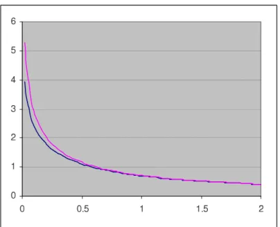
ρ = E · 1 eβc(1+εω)− 1 ¸ . (4.7)
Remark that, irrespective of the distribution of εω, the equation (4.7) implies that the
resulting βc is lower than ln
³
1 + 1ρ´, which corresponds to the nonrandom case εω
x = 0, i.e.
disorder enhances Bose-Einstein condensation. We shall see (Sect.4.3.3) that this is no longer true when λ > 0, and even that the opposite holds, if λ is small enough!
Notice that formula (4.7) is in agreement with the general expression found in [L-Z]: ρ =
Z d ¯ N (E)
eβcE − 1, (4.8)
where ¯N (E) is the integrated density of states given by ¯
N (E) = a.s.− lim
V →∞
1
V#{i : E
ω
Here {Eω
i }i≥1 are the eigenvalues of the one-particle Hamiltonian with a random potential
{εω x}x∈Λ: (hω Λu)(x) := (tΛu)(x) + X x∈Λ εω xu(x) , x∈ Λ, u ∈ h(Λ), (4.10)
for i.r. kinetic-energy hopping, see (2.1), (2.10), and #{i : Eω
i ≤ E} counting the number of
the corresponding eigenfunctions (including the multiplicity). It is known that for any ergodic random potential {εω
x}x∈Λ, the limit (4.9) exists almost surely (a.s.) and that it is non-random,
see e.g.[PF]. A contact between formulae (4.7) and (4.8) gives the following
Lemma 4.1 The integrated density of states is equal to ¯
N (E) = P [εω ≤ E − 1] = E [θ(E − (1 + εω))] . (4.11) Proof : For simplicity we consider the case of a Bernoulli random potential {εω
x}x∈Λ such that
εω
x = ε with probability p and εωx = 0 with probability 1− p. (The proof of the general case
is similar, but slightly more complicated.) In this special case, the right-hand side of (4.11) equals P[εω ≤ E − 1] = 1 if E ≥ 1 + ε, 1− p if 1 ≤ E < 1 + ε, 0 if E < 1. (4.12) Clearly, all eigenvalues {Eω
i }i≥1 of the Hamiltonian (4.10) belong to the interval [1, 1 + ε].
Since dim(h(Λ)) = V , one gets ¯N (E) = 1, if E ≥ 1 + ε. Similarly, ¯N (E) = 0, if E < 1. Now suppose that E ∈ [1, 1 + ε). Since {εω
x}x∈Λ is the Bernoulli random field, for given
δ > 0, there exists c > 0 such that with probability P r > 1− δ the number of sites x ∈ Λ with εω
x = ε is in the interval (pV − c
√
V , pV + c√V ). Given a configuration for which this is the case, let Λε ⊂ Λ be the set where εωx = ε. Consider the states φ∈ h(Λ) such that φ(x) = 0, if
x /∈ Λε and Px∈Λφ(x) = 0. Then (hωΛφ)(x) = 1 V V X y=1 (φ(x)− φ(y)) + εωxφ(x) = (ε + 1)φ(x) , x∈ Λε.
The space of such eigenfunctions φ has dimension |Λε| − 1, so that
#{Eiω > E} ≥ (|Λε| − 1).
Since (#{Eω
i ≤ E}) + (#{Eiω > E}) = V , for V → ∞ we get
¯
N (E) ≤ 1 − p.
Similarly, considering the eigenfunctions with supports concentrated on Λc
ε = Λ\ Λε we obtain
¯
N (E) ≥ 1 − p.
Together with (4.12) these estimates give the proof of (4.11). ¤
The relations (4.11) show that the formulae (4.7) and (4.8) are equivalent. For details of a general statement see e.g. [PF] Ch.II.5 .
4.2
Discrete random potential and
λ > 0
We now consider the case with interaction λ > 0, and first assume that the probability distri-bution of εω
x is discrete.
A particularly simple case corresponds to the hard-core boson limit λ = +∞, see Section 3. Then by (3.21) the equations for the critical value of the inverse temperature βc:= βc(ρ) =
βc(ρ, λ = +∞) for a given density ρ, reduce to the system:
E· tanh β(µ− ε ω− 1)/2 µ− εω− 1 ¸ = 1 (4.13) and ρ = 1 2 + 1 2E · tanh1 2β(µ− ε ω − 1) ¸ . (4.14)
The last equation (4.14) implies that for the hard-core interaction the total particle density has the estimate: ρ ≤ 1.
4.2.1 Bernoulli random potential in the hard-core limit λ = +∞. A special case of a discrete distribution is the Bernoulli distribution, where εω
x = ε with
proba-bility p and εω
x = 0 with probability 1− p. We first consider the case λ = +∞. The equations
(4.13) and (4.14) then read, Fp,ε(β = βc, µ) := p tanh1 2βc(µ− ε − 1) µ− ε − 1 + (1− p) tanh1 2βc(µ− 1) µ− 1 = 1 (4.15) and Gp,ε(β = βc, µ) := 1 2+ 1 2 · p tanh1 2βc(µ− ε − 1) + (1 − p) tanh 1 2βc(µ− 1) ¸ = ρ. (4.16) Here a new phenomenon occurs for density ρ = 1− p. To see this, we consider first a particular case of p = 1/2. Then ρ = 1/2, and by (4.16) we obtain, that the only possible solution for the corresponding chemical potential is µ(ρ = 1/2) := µ(ρ = 1/2, λ = +∞) = 1 + ε/2. Inserting this value of µ into (4.15) we get for the critical temperature:
tanhβcε
4 =
1 2ε .
This equation obviously has no solution for ε ≥ 2. Therefore, there is no Bose-Einstein con-densation for Bernoulli random potential, if p = ρ = 1/2, and ε is greater than some critical value: εcr = 2.
One can check that the same phenomenon occurs for p6= 1/2 and for densities ρ = 1 − p, if ε is large enough, but now the reasoning is more delicate. First of all, by (4.15) and tanh u≤ u we see that in any case there is a lower bound on the inverse critical temperature:
βc≥ 2. (4.17)
Now assume that p < 1/2, i.e. ρ > 1/2. From (4.16) it then follows that for any ε one has 0 < µ− 1 − 1
Indeed, if we suppose that 0 ≤ µ − 1 ≤ ε/2, then tanh1 2βc(µ− 1) ≤ tanh 1 2βc(1 + ε− µ) and hence, by (4.16), we get 2ρ− 1 = p tanh1 2βc(µ− ε − 1) + (1 − p) tanh 1 2βc(µ− 1) ≤ (1 − 2p) tanh1 2βc(ε + 1− µ) < 1 − 2p , contradicting our assumption ρ = 1− p, if βc exists and is finite.
Now notice that (4.16) with ρ = 1− p is equivalent to 1− tanh1 2βc(ε + 1− µ) 1− tanh1 2βc(µ− 1) = 1− p p . (4.19)
The left-hand side of (4.19) can be estimated from below as 1− tanh1 2βc(ε + 1− µ) 1− tanh1 2βc(µ− 1) = e βc(µ−1−ε/2)+ e−βcε/2 e−βc(µ−1−ε/2)+ e−βcε/2 > e βc(µ−1−ε/2) .
Together with (4.17) this yield an upper bound for (4.18): 0 < µ− 1 − 1 2ε < 1 βc ln1− p p ≤ 1 2ln 1− p p < 1− 2p 2p . (4.20)
But (4.20) implies that (4.15) has no solution βc, since for large ε we obtain
ptanh 1 2βc(µ− ε − 1) µ− ε − 1 + (1− p) tanh1 2βc(µ− 1) µ− 1 < (4.21) p ε + 1− µ + 1− p µ− 1 < p ε/2− (1 − 2p)/2p + 1− p ε/2 < 1 . We assumed that p < 1/2. Therefore by (4.21), our conclusion is true, in fact, for
ε≥ 1/p ≥ 2 = εcr . (4.22)
The same result follows in the case p ≥ 1/2, if we interchange p and 1−p and µ−1 and 1+ε−µ in the above argument.
Next we show that for any other ρ∈ (0, 1), i.e. for any ρ 6= 1 − p, the critical βc(ρ) < +∞,
i.e. for these densities one always has the Bose-Einstein condensation at low temperatures. To this end suppose that there is ρ∗ ∈ (0, 1) such that ρ∗ 6= 1 − p, but lim
ρ→ρ∗βc(ρ) = +∞.
Then the left-hand side of (4.15) converges to lim β→∞Fp,ε(β, µ) = Mp(µ, ε) := p |µ − ε − 1| + 1− p |µ − 1| . (4.23)
The number of solutions of equation (4.15) in the limit limρ→ρ∗βc(ρ) = +∞ depends on the
value of ε > 0, but two singular points µ = 1 and µ = 1 + ε of the function (4.23) ensure (for nontrivial values of the probability: p 6= 0 and p 6= 1) that there are always at least two solutions: µ1(ε) < 1 and µ2(ε) > 1 + ε of equation
If limρ→ρ∗βc(ρ) = +∞, then for these two cases the equation (4.16) implies:
ρ∗ = lim
ρ→ρ∗Gp,ε(βc(ρ), µ1(ε) = 0 ,
ρ∗ = lim
ρ→ρ∗Gp,ε(βc(ρ), µ2(ε) = 1 .
This contradicts our assumptions on ρ∗ and makes impossible the hypothesis lim
ρ→ρ∗βc(ρ) =
+∞.
Notice that the function Mp(µ, ε) has a minimum µ(ε) ∈ (1, 1 + ε). If Mp(µ(ε), ε) < 1
(which is equivalent to ε > εp := 1 + 2pp(1 − p)), then equation (4.24) has two complementary
solutions µ∓(ε): µ∓(ε) = ε + 3 2 − p ∓ s µ ε− 1 2 ¶2 − p(1 − p) , (4.25) such that 1 < µ−(ε) < µ(ε) < µ+(ε) < 1 + ε .
If limρ→ρ∗βc(ρ) = +∞, then for these two solutions equation (4.16) implies:
ρ∗ = lim
ρ→ρ∗Gp,ε(βc(ρ), µ∓(ε)) = 1− p ,
This again contradicts our assumption about ρ∗, and thus proves the assertion: β
c(ρ) < +∞
for any ρ 6= 1 − p.
Notice that by (4.25) the equation Mp(µ(ε), ε) = 1 has a unique solution ε = εp ≤ εcr = 2,
and one obtains Mp(µ(ε), ε) > 1 for all ε < εp, which excludes complementary solutions µ∓(ε).
On the other hand, if
ε > εcr = max
p εp = εp=1/2 , (4.26)
there are always complementary solutions (4.25). This may restrict the values of ρ, for which we have bounded critical βc(ρ), to a certain domain of densities.
To this end we consider first the ρ -independent equation (4.15). Notice that Fp,ε(β, µ) is a
monotonously increasing function of β, so there is a unique solution ˜βc(µ) of equation (4.15)
for a given µ, if there is one.
Since (tanh u)/u ≤ 1, then the left-hand side of (4.15) is less than 1, for β ≤ 2. On the other hand, as β → ∞, the left-hand side of (4.15) converges to Mp(µ, ε). Since the function
(4.23) is singular at µ = 1 and µ = 1 + ε, a solution 2 < ˜βc(µ) < +∞ for a certain µ always
exists, and the set of those µ is defined by the condition: Sp,ε :={µ ∈ R1 : lim
β→∞Fp,ε(β, µ) = Mp(µ, ε) ≥ 1} (4.27)
By (4.23) the set (4.27) for ε > 0 is a compact in R1
+. If there are no complementary solutions
µ∓(ε), this compact is connected, but if
ε > εcr . (4.28)
it contains two domains separated by a gap:
see (4.25). The gap I(ε, p)⊂ (1, 1 + ε). There is no solutions ˜βc(µ) for µ ∈ I(ε, p) and for µ < (ε + 1)/2− q ((ε− 1)/2)2− ε(1 − p) , or for µ > (ε + 3)/2 + q ((ε + 1)/2)2− ε(1 − p) .
Hence, for large ε (4.28) the set Sp,ε is a union of two (separated by the gap I(ε, p)) bounded
domains, which are vicinities of singular points µ = 1 and µ = 1 + ε . is in fact not the To understand, how the gap in the chemical potential for solution ˜βc(µ) modify the
behav-iour of βc(ρ), we have to consider the ρ -dependent equation (4.16). Notice that from (4.16)
one obtains ˆβc(µ, ρ) as a function of two variables. Therefore, βc(ρ) is a solution of equation:
˜
βc(µ) = ˆβc(µ, ρ) , (4.29)
which in fact connects µ and ρ: µ(ρ), i.e. βc(ρ) = ˜βc(µ(ρ)) = ˆβc(µ(ρ), ρ).
Clearly, the left-hand side Gp,ε(β, µ) is increasing in µ and it tends to 0 as µ → −∞ and to
1 as µ → +∞. Excluding ρ = 0 or 1, there is therefore a unique solution µ(β, ρ) of (4.16) for each value of β. As β → 0, Gp,ε(β, µ) tends to 1/2 at constant µ. Therefore, if ρ6= 1/2
lim
β→0µ(β, ρ) =±∞ ,
depending on whether ρ > 1/2 or ρ < 1/2.
On the other hand, in the limit β → ∞, we have that Gp,ε(β, µ): (a) tends to 0, if µ < 1;
(b) to (1− p)/2, if µ = 1; (c) to 1 − p, if 1 < µ < 1 + ε; (d) to 1 − p/2, if µ = 1 + ε, and (e) to 1, if µ > 1 + ε.
The (a)− (e) give relation between ρ and µ for large β : if 0 < ρ < 1 − p, we must have µ(β, ρ) → 1 and, if 1 − p < ρ < 1, we obtain µ(β, ρ) → 1 + ε, for β → ∞. At ρ = 1 − p, we have to use the representation (4.19), that yields
µ(β, ρ = 1− p) = 1 +1 2ε− 1 2βln p 1− p+ o(β−1) , (4.30)
if β is large. In particular, this justifies the remark (4.22) above about εcr = 2, since 1 + ε/2
lies in the gap I(ε, p) only if ε≥ 2 = εcr, see (4.25).
Hence, it follows that for ρ 6= 1 − p two functions of µ corresponding to solutions (4.29) of equations (4.15), (4.16) must intersect. On the other hand, (4.22) proves that they can not intersect for ρ = 1− p , if ε > εcr. In fact, we can derive upper bounds for βc(ρ) in the case
ρ 6= 1 − p and |ρ − 1 + p| small.
To this end we first consider the case ρ > 1− p. Let us assume p ≤ 1/2. (The case p > 1/2 can be studied similarly.) Writing ρ = 1− p + δ/2 we present the equation (4.16) in the form
p tanh1
2βc(ε + 1− µ) = (1 − p) tanh 1
2βc(µ− 1) + 2p − 1 − δ . (4.31) Identity (4.31) implies that µ > 1 + ε/2, since otherwise we get a contradiction:
1− 2p + δ = −p tanh1 2βc(ε + 1− µ) + (1 − p) tanh 1 2βc(µ− 1) ≤ −p tanh1 2βc(ε + 1− µ) + (1 − p) tanh 1 2βc(ε + 1− µ) ≤ 1 − 2p .
On the other hand, for ε ≥ 1, one gets the upper limit µ < ε + 1. Indeed, if we suppose the opposite: µ ≥ ε + 1, then (4.16) and the general fact that βc≥ 2 (see (4.17)) yield
1− 2p + δ = p tanh1 2βc(µ− ε − 1) + (1 − p) tanh 1 2βc(µ− 1) ≥ (1 − p) tanh1 2βc(µ− 1) ≥ (1 − p) tanh ε. But this is impossible for (large) ε verifying:
ε > 1 2ln
2− 3p + δ
p− δ . (4.32)
Therefore, we obtain for µ the lower and upper bounds:
1 + ε/2 < µ < 1 + ε . (4.33)
Now identity (4.31), together with the bounds (4.33), inequality tanh(u) > 1− 2e−2u and
βc ≥ 2 (see (4.17)), yields the estimates:
1− δ p − 2 pe −ε < tanh1 2βc(ε + 1− µ) < 1 − δ p. (4.34) 1 > p− δ − 2e −ε ε + 1− µ + (1− p) 1− 2e−ε µ− 1 > βc(p− δ − 2e−ε) ln(2p/δ) and hence, βc < 1 p− δ − 2e−εln(2p/δ). (4.35)
The upper bound (4.35) holds for example, if δ < p/2 and ε > ln(4/p).
Now we consider the case ρ < 1− p and suppose p ≤ 1/2, since p > 1/2 can be studied similarly. Then we write: ρ = 1− p − δ/2. Equation (4.16) now reads as
(1− p) tanh1
2βc(µ− 1) = p tanh 1
2βc(1 + ε− µ) + 1 − 2p − δ . (4.36) An argument similar to the case ρ > 1− p shows that
1 < µ < 1 + ε , (4.37)
if ε is large enough and δ < 1− p. Indeed, if we suppose the opposite: µ ≥ 1 + ε, then 1− 2p − δ ≥ (1 − p) tanh1
2βc(µ− 1) ≥ (1 − p) tanh ε , which is impossible for
ε > 1 2ln
2− 3p − δ p + δ . Similarly, if we suppose that µ≤ 1, then (4.36) implies
0 > p tanh1
which is impossible if δ < 1− 2p , or if 1 − 2p ≤ δ < 1 − p and ε > 1
2ln
3p− 1 + δ 1− p − δ . Now, (4.36) and (4.37) imply that
tanh1
2βc(µ− 1) < 1 − δ
1− p . (4.38)
In the case µ≥ 1 + 1
2ε this yields immediately the upper bound :
βc <
2 ε ln
2(1− p)
δ . (4.39)
On the other hand, if 1 < µ < 1 + ε/2, then by (4.36) and βc ≥ 2 we obtain
(1− p) tanh1 2βc(µ− 1) > p tanh 1 4βcε + 1− 2p − δ > p tanh1 2ε + 1− 2p − δ > p(1 − 2e −ε) + 1− 2p − δ = 1 − p − δ − 2pe−ε . (4.40)
Taking into account equation (4.15) and estimates (4.38), (4.40), we get 1 > 1− p − δ − 2pe−ε
µ− 1 > βc
1− p − δ − 2pe−ε
ln(2(1− p)/δ) , that gives the upper bound:
βc<
1
1− p − δ − 2pe−εln
2(1− p)
δ . (4.41)
4.2.2 Bernoulli random potential for the case λ < +∞.
We assume in this subsection that λ > ε + 1. If the repulsion is very large (λ ≫ ε + 1), the analysis for ρ < 1 is then almost the same as above for λ = +∞, whereas for ρ ≥ 1, which is possible only for finite λ, one needs some more arguments.
Here we start with the estimate the first-order correction in λ−1 to the value of ε cr(λ =
+∞) = 2. With this accuracy the equations (4.5) and (4.6) can be approximated correspond-ingly by p µtanh1 2β(µ− ε − 1) µ− ε − 1 + 1 2λ + ε + 1− µ e−β(1+ε−µ)/2 cosh1 2β(1 + ε− µ) ¶ (4.42) +(1− p) µtanh1 2β(µ− 1) µ− 1 + 1 2λ + 1− µ eβ(µ−1)/2 cosh1 2β(µ− 1) ¶ = 1 , and by (4.16) as above.
To see this, note that if ρ < 1, the dominant contribution in (4.6) must come from the n = 1 term, i.e. we must have h1 < h2, so µ < 1 + 2λ + ε. The other terms in (4.6) are then
Now, because of the presence of e−βh1 in the n = 2 term of (4.4), it cannot be neglected in (4.5) and we obtain: 2p 1 + e−β(1+ε−µ) ½ e−β(1+ε−µ)− 1 µ− 1 − ε + 2 e−β(1+ε−µ) 1 + 2λ + ε− µ ¾ + 2(1− p) 1 + e−β(1−µ) ½ e−β(1−µ)− 1 µ− 1 + 2 e−β(1−µ) 1 + 2λ− µ ¾ = 2 , which is the same as (4.42).
Similar to (4.23) the gap equation for 1 < µ < 1 + ε can be obtained from (4.42) in the limit β → ∞: p ε + 1− µ + (1− p) µ 1 µ− 1+ 2 2λ + 1− µ ¶ = 1. (4.43)
If ρ = 1 − p, then by (4.16) and (4.30) we again obtain the limit: µ → 1 + 1
2ε for β → ∞.
Inserting this limit into (4.43) we obtain 2 ε + 2(1− p) 2λ− 1 2ε = 1 . (4.44)
Hence, by the reasoning similar to those after (4.30), we obtain the critical value of the Bernoulli random potential εcr(λ) the expression:
εcr(λ)≈
2
1− (1 − p)/λ = 2 + 2(1− p)/λ + . . . , (4.45) which takes into account that λ is large but finite.
Another observation, which is related to the finiteness of λ, concerns the value βc(ρ = 1).
For hard-core bosons the arguments in the Sect.4.2.1 show that this value is infinite and the corresponding values of the chemical potential must be greater than 1 + ε, see (4.6). Now for finite λ and µ > 1 + ε the limit of (4.42), when β → ∞, reads as:
p µ 1 µ− ε − 1 + 2 2λ + 1 + ε− µ ¶ + (1− p) µ 1 µ− 1 + 2 2λ + 1− µ ¶ = 1. (4.46)
If ρ≥ 1, then we need to reconsider the density equation (4.6), which has the form: ρ = p P∞ n=1n e−βhn(µ−ε,λ) P∞ n=0e−βhn(µ−ε,λ) + (1− p) P∞ n=1n e−βhn(µ,λ) P∞ n=0e−βhn(µ,λ) . (4.47)
Notice that if β → +∞, then by (4.2) and (4.47) one obtains the following limits: ρ → 1, when µ ∈ (1 + ε, 1 + 2λ) , ρ → 2 − p, when µ ∈ (1 + 2λ, 1 + 2λ + ε), and ρ → 2, when µ∈ (1 + 2λ + ε, 1 + 4λ).
and write in this limit: 1 ≈ p ½ e−β(1+ε−µ)+ 2e−2β(1+λ+ε−µ) 1 + e−β(1+ε−µ)+ e−2β(1+λ+ε−µ) ¾ +(1− p) ½ e−β(1−µ)+ 2e−2β(1+λ−µ) 1 + e−β(1−µ)+ e−2β(1+λ−µ) ¾ = p ½ 1 + 2e−β(1+ 2λ+ε−µ) 1 + e−β(µ−1−ε)+ e−β(1+2λ+ε−µ) ¾ +(1− p) ½ 1 + 2e−β(1+2λ−µ) 1 + e−β(µ−1)+ e−β(1+2λ−µ) ¾ (4.48) ≈ 1 + p¡e−β(1+2λ+ε−µ)− e−β(µ−1−ε)¢ +(1− p)¡e−β(1+2λ−µ)− e−β(µ−1)¢ . This yields e2βµ≈ e2β(1+λ) 1− p + pe βε 1− p + pe−βε ≈ p 1− pe 2β(1+λ+1 2ε).
The chemical potential defined by equation (4.47) therefore tends (for ρ = 1) to 1 + λ + 12ε as
β → +∞.
Therefore, inserting this into (4.46) we obtain the estimate for the value of repulsion λc,1
that ensures that βc(ρ = 1) = +∞ in the presence of the random Bernoulli potential:
λc,1(ε) = 1 2 " 3 + r 9 + 2ε(1− 2p + 1 2ε) # . (4.49)
Remark 4.1 In the absence of disorder, i.e. if ε = 0, the critical value of lambda is λc,1 = 3
as opposed to λ1 = 12(3 +
√
8) as suggested in [BD]. The reason is the same as above for εcr,
namely, the graph of µ(β, ρ) at ρ = 1 tends to 1 + λ as β → +∞ and this lies in the gap only if λ ≥ 3. Similarly, the next critical values are given by
λc,k(ε = 0) = 2k + 1. (4.50)
Remark 4.2 In Sect.4.2.1 we notice a new phenomenon specific for the random case: diver-gence of βc at ρ = 1− p for hard-core bosons, cf. Figure 1 for p = 1/2. Instead of fixing λ,
fixing ε > 2 it follows from (4.44) that there is a critical value of the repulsion λc,1−p(ε) (instead of ε as in (4.45)) so that βc(ρ = 1− p) diverges for λ ≥ λc,1−p(ε) in the presence of the random
Bernoulli potential:
λc,1−p(ε) = ε 4+
ε(1− p)
ε− 2 . (4.51)
This critical value is not evident from Figure 1 as ε = 2.
Remark 4.3 In Sect.4.1 we remarked that the critical temperature for free bosons increases due to disorder. We also remarked that for the interacting case this is a more subtle matter, since it depends on the value of repulsion. For large repulsions close to e.g. λc,1(ε = 0) = 3,
we get by (4.49) that
This lowering of βc(ρ = 1) can be explained intuitively as follows. At density ρ = 1, there is
one particle per site. If ε = 0 there is a penalty for a particle to jump to an already occupied site, so the preferred state is where the particles are at fixed sites, which is almost an eigenstate of the number operators nx for each site. This prevents Bose condensation. (This argument
was presented also in [BD].) However, if ε > 0, then the lattice splits into two parts with energies 0 and ε, and a particle jumping from a site with energy ε to a site with energy 0 loses an energy ε, which counteracts the gain of λ. This creates more freedom of movement and therefore promotes Bose condensation. On the other hand, for a fractional value of the ρ in the neighbourhood of ρ = 1− p, the critical temperature decreases with increasing ε as can be seen from Figure 1.
Now consider the case ρ > 1. From equation (4.47) we see that at fixed ρ ∈ (1, 2 − p), µ→ 1 + 2λ and for ρ ∈ (2 − p, 2), µ → 1 + 2λ + ε as β → ∞.
For the case ρ = 2− p, we have to expand (4.47), as above for ρ = 1, see (4.48), but to take into account that µ ∈ (1 + 2λ, 1 + 2λ + ε):
ρ ≈ p ½ 1 + 2e−β(1+ 2λ+ε−µ) 1 + e−β(µ−1−ε)+ e−β(1+2λ+ε−µ) ¾ (4.53) +(1− p) ½ eβ(1+2λ−µ)+ 2 1 + eβ(1+2λ−µ)+ e−2β(µ−1−λ) ¾ ≈ 2 − p + p¡e−β(1+ε+2λ−µ)− e−β(µ−1−ε)¢ − (1− p)e−β(µ−1−2λ)− 2(1 − p)e−2β(µ−1−λ).
This yields that e−β(µ−1−2λ) ≈ e−β(1+ε+2λ−µ)p/(1 − p) for large β, i.e. µ → 1 + 2λ + 1 2ε, if
ρ = 2− p and β → ∞. For µ ≈ 1 + 2λ + 1
2ε, one has h1(µ− ε, λ) < h2(µ− ε, λ). So that the p-terms in (4.42)
are unchanged, but h1(µ, λ) > h2(µ, λ) < h3(µ, λ), if λ > ε/4, which corresponds to our initial
hypothesis about the value of repulsion: λ > 1 + ε. Hence, the (1−p)-terms are now dominated for large β by n = 2 and (4.42) read as
p 1 + e−β(1+ε−µ) ½ e−β(1+ε−µ)− 1 µ− 1 − ε + 2 e−β(1+ε−µ) 1 + 2λ + ε− µ ¾ + 1− p e−β(1−µ)+ e−2β(1−µ+λ) ½ 2 e−2β(1−µ+λ)− e−β(1−µ) µ− 1 − 2λ + 3 e−2β(1−µ+λ) 1 + 4λ− µ ¾ ≈ 1, In the limit β → ∞ we obtain from this relation the gap equation
p µ 1 µ− 1 − ε + 2 1 + ε + 2λ− µ ¶ + (4.54) (1− p) µ 2 µ− 1 − 2λ + 3 1 + 4λ− µ ¶ = 1 . Inserting µ = 1 + 2λ + 12ε into (4.54) leads to
1 2ε 2 − (2λ − 1 + 2p)ε + 8λ = 0. (4.55) Solutions of (4.55) are: εcr,±(2) = (2λ− 1 + 2p) ±p(2λ − 1 + 2p)2 − 16λ . (4.56)
Hence, there is a solution that for large λ has the form: ε(2) cr (λ) = 4 µ 1 + 1− 2p 2λ ¶ + . . . , (4.57)
or other way around, for a given ε we have:
λc,ρ=2−p(ε) = 2(2p− 1)
(ε− 4) . (4.58)
Clearly, this critical value only applies if ε > 4 and p > 1/2. The top graph of Figure 1 illustrates this behaviour at ρ = 1.5 for ε = 4.5 and λ = 10.
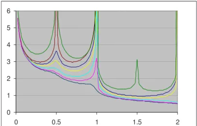
The critical βc(ρ) for the Bernoulli distribution with p = 1/2 and ε = 2 is shown in Figure
1 for a number of values of λ. Notice in particular that ε < εcr(λ), see (4.45), for all finite λ,
so that βc(ρ = 1/2) < +∞.
Also, for λ = 3.3, one obtains βc(ρ = 1) < +∞ because 3.3 < λc,1(ε = 2) = (3 +
√ 13)/2, see (4.49).
Figure 1: βc as a function of the density ρ in the case of
aver-aging over two energies: 0 and ε = 2 with equal probabilities, for various values of λ: λ = 3, 3.3, 4, 6, 10 and +∞. The top graph corresponds to the case ε = 4.5 and λ = 10.
4.2.3 Trinomial distribution: λ = +∞.
We also briefly consider the trinomial distribution, taking for simplicity equal probabilities, i.e. εω = 0 Pr = 1/3 1 2ε Pr = 1/3 ε Pr = 1/3 . (4.59) For hard-core bosons, λ = +∞, equation (4.13) for the critical value of βc(ρ) takes the form:
1 3 ·tanh1 2β(µ− 1) µ− 1 + tanh1 2β(µ− 1 − 1 2ε) µ− 1 − 1 2ε + tanh 1 2β(µ− 1 − ε) µ− 1 − ε ¸ = 1 . (4.60)
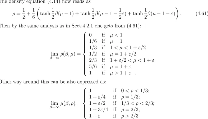
The density equation (4.14) now reads as ρ = 1 2 + 1 6 µ tanh1 2β(µ− 1) + tanh 1 2β(µ− 1 − 1 2ε) + tanh 1 2β(µ− 1 − ε) ¶ . (4.61)
Then by the same analysis as in Sect.4.2.1 one gets from (4.61):
lim β→∞ρ(β, µ) = 0 if µ < 1 1/6 if µ = 1 1/3 if 1 < µ < 1 + ε/2 1/2 if µ = 1 + ε/2 2/3 if 1 + ε/2 < µ < 1 + ε 5/6 if µ = 1 + ε 1 if µ > 1 + ε . Other way around this can be also expressed as:
lim β→∞µ(β, ρ) = 1 if 0 < ρ < 1/3; 1 + ε/4 if ρ = 1/3; 1 + ε/2 if 1/3 < ρ < 2/3; 1 + 3ε/4 if ρ = 2/3; 1 + ε if ρ > 2/3.
Again, similar to the reasoning in Sect.4.2.1, the inserting of µ = 1 + ε/4 or µ = 1 + 3ε/4 into the limiting equation (4.60) for β → +∞ yields the critical value of the random potential:
εcr=
28
9 . (4.62)
Therefore, (similar to the Bernoulli case for ρ = 1/2) the condensation of hard-core bosons is absent at densities ρ = 1/3 and ρ = 2/3, if ε ≥ εcr. This phenomenon of course persists for
λ < +∞ and there are similar suppressions of Bose condensation at ρ = 4/3, 5/3, etc., if ε is large enough.
4.2.4 Trinomial distribution: λ < +∞.
For λ < +∞ there is a similar enhancement of Bose condensation at ρ = 1 as for the Bernoulli distribution, but the effect is stronger. This can be seen in Figure 2. The explanation is similar to that in Remark 4.3, except now the lattice splits into 3 equal parts with energies 0, ε/2 and ε. Particles can jump from a singly-occupied site with energy ε to a singly-occupied site with energy 0 or ε/2, thus compensating for the energy penalty of λ due to double occupation.
By equation (4.14) for (4.59) we obtain that at ρ = 1, µ(β, ρ)→ 1 + λ + ε/2 as β → +∞. The gap equation (4.60) then reduces to
1 λ− ε/2 + 1 λ + 1 λ + ε/2 = 1 . We can solve it for ε provided λ ≥ 3:
εcr(λ) = 2λr λ − 3
λ− 1 . (4.63)
Thus, Bose condensation is absent, if λ≥ 3 and ε ≤ εcr(λ).
Figure 2 shows βc(ρ) for a fixed ε = 10 and for values of λ≥ 3. Then ε ≥ εcr(λ = 3, 4, 6),
Figure 2: βc as a function of the density ρ in the case of a
trinomial distribution with width ε = 10 for λ = 3, 4, 6 and 8.
4.2.5 General discrete distribution.
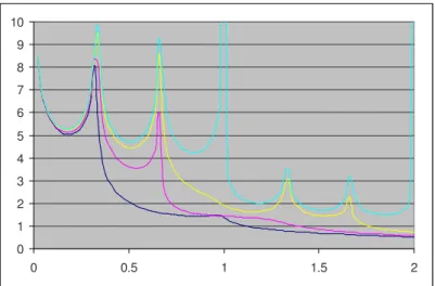
The same phenomena persist for higher numbers of random potential energy values, but the critical value εcr(λ) becomes rapidly very large. Figure 3 shows the case of a distribution with
equals probabilities Pr = 1/10 at 10 equidistant values of εω (with maximal value ε = 10)
for λ = 8. Clearly, condensation is suppressed at ρ = 1/10, . . . , 9/10 and ρ = 1, 2 but not at corresponding fractional values above 1, cf. Figure 2.
Figure 3: βc as a function of the density ρ in the case of
4.3
Continuous distribution
4.3.1 The case λ = +∞.
Consider a random potential with homogeneous distribution between 0 and ε. In case λ = +∞ the equations (4.13) and (4.14) become
1 ε Z ε 0 tanh1 2β(µ− 1 − x) µ− 1 − x dx = 1 (4.64) and 1 ε Z ε 0 tanh1 2β(µ− 1 − x)dx = 2ρ − 1 . (4.65)
The latter has sense only for 0 ≤ ρ ≤ 1 and can be solved exactly for µ: 2 βεln eβ(µ−1)/2+ e−β(µ−1)/2 eβ(µ−1−ε)/2+ e−β(µ−1−ε)/2 = 2ρ− 1 , and hence µ(β, ρ) = 1 + 1 2ε + 1 βln sinh12βρε sinh12β(1− ρ)ε . (4.66)
As β → +∞, the expression (4.66) takes the form lim
β→+∞µ(β, ρ) := µ(ρ) = 1 + ερ , 0 < ρ < 1 , (4.67)
whereas µ(ρ = 0)∈ (−∞, 1] and µ(ρ = 1) ∈ [1 + ε, +∞) for extreme values of density, i.e., the inverse function is ρ(µ) = 0 µ≤ 1 (µ− 1)/ε 1 < µ < 1 + ε 1 1 + ε≤ µ . (4.68) Then by (4.64) and (4.68) we obtain for ρ = 1 in the limit β → +∞:
1 = 1 ε Z ε 0 1 µ− 1 − xdx , or we get explicitly the value of the chemical potential
µ(ρ = 1) = 1 + ε
1− e−ε > 1 + ε ,
and similarly
µ(ρ = 0) = 1− εe−ε
1− e−ε < 1 .
Hence, for hard-core bosons the critical βc(ρ) is infinite at extreme densities ρ = 0, 1 for any
value ε > 0 of the uniform continuous distribution.
If 0 < ρ < 1, then solution of the equation (4.65) in the limit β → +∞ is (4.67), whereas the integral in (4.64) diverges. Therefore, if the critical βc(0 < ρ < 1) exist, it must be bounded.
Moreover, since (tanh u)/u ≤ 1, by (4.64)we get for it a bound from below: 2 < βc(0 < ρ < 1).
To prove the existence and uniqueness of βc(0 < ρ < 1) consider first (4.65) for ρ≤ 12. Then
![Figure 3 shows the phase diagram for λ = 10 with ε = 3, taking an average over a uniform distribution corresponding to 10 equidistant random values of ε ω in the interval [0, 3]](https://thumb-eu.123doks.com/thumbv2/123doknet/14618740.733481/33.892.241.644.389.654/figure-diagram-average-uniform-distribution-corresponding-equidistant-interval.webp)