HAL Id: hal-01779631
https://hal-amu.archives-ouvertes.fr/hal-01779631
Submitted on 27 Apr 2018
HAL is a multi-disciplinary open access
archive for the deposit and dissemination of
sci-entific research documents, whether they are
pub-lished or not. The documents may come from
teaching and research institutions in France or
abroad, or from public or private research centers.
L’archive ouverte pluridisciplinaire HAL, est
destinée au dépôt et à la diffusion de documents
scientifiques de niveau recherche, publiés ou non,
émanant des établissements d’enseignement et de
recherche français ou étrangers, des laboratoires
publics ou privés.
Adaptive and Opportunistic Exploitation of
Tree-decompositions for Weighted CSPs
Philippe Jégou, Hélène Kanso, Cyril Terrioux
To cite this version:
Philippe Jégou, Hélène Kanso, Cyril Terrioux. Adaptive and Opportunistic Exploitation of
Tree-decompositions for Weighted CSPs. 2017 International Conference on Tools with Artificial Intelligence
(ICTAI 2017), Nov 2017, Boston, MA, United States. �hal-01779631�
Adaptive and Opportunistic Exploitation of
Tree-decompositions for Weighted CSPs
Philippe J´egou
H´el`ene Kanso
Cyril Terrioux
Aix-Marseille Univ, Universit´e de Toulon, CNRS, ENSAM, LSIS, Marseille, France {philippe.jegou, hanan.kanso, cyril.terrioux}@lsis.org
Abstract—When solving weighted constraint satisfaction
prob-lems, methods based on tree-decompositions constitute an in-teresting approach depending on the nature of the considered instances. The exploited decompositions often aim to reduce the maximal size of the clusters, which is known as the width of the decomposition. Indeed, the interest of this parameter is related to its importance with respect to the theoretical complexity of these methods. However, its practical interest for the solving of instances remains limited if we consider its multiple drawbacks, notably due to the restrictions imposed on the freedom of the variable ordering heuristic.
So, we first propose to exploit new decompositions for solving the constraint optimization problem. These decompositions aim to take into account criteria allowing to increase the solving efficiency. Secondly, we propose to use these decompositions in a more dynamic manner in the sense that the solving of a subprob-lem would be based on the decomposition, totally or locally, only when it seems to be useful. The performed experiments show the practical interest of these new decompositions and the benefit of their dynamic exploitation.
Index Terms—Weighted CSP; solving; decomposition
I. PRELIMINARIES
The Weighted Constraint Satisfaction Problem (WCSP) offers a general framework that permits to model and solve efficiently many real problems like, for example, the frequency allocation problem [1] or some problems related to bioinfor-matics [2]. In this paper, our main goal is to improve the efficiency of the structural solving methods, namely those based on tree-decompositions. First, we recall the definition of a WCSP instance:
Definition 1: A WCSP instance is defined as a triplet (X, D, W )with:
• X = {x1, . . . , xn} is a set of n variables,
• D = {Dx1, . . . , Dxn} is a set of finite domains of values
where each domain Dxi is related to the variable xi,
• W is a set of e cost functions. A cost function that involves the set {xi1, xi2, . . . , xik} of variables is a
function that associates to each tuple of Dxi1 × Dxi2× . . .× Dxik a given integer between 0 and k with k the maximal cost corresponding to a completely forbidden tuple (expressing hard constraints).
For the sake of simplicity, our presentation is restricted to binary instances, that is the instances for which each cost func-tion involves at most two variables. However, our work can be easily extended to non-binary instances. In particular, we use both binary and non-binary instances in the experimentations. In the following, wij denotes the cost function involving
the variables xi and xj, wi denotes the unary cost function corresponding to xi and w∅ denotes the zero arity constraint which represents a constant cost paid by any assignment. The cost of a complete assignment (v1, . . . , vn)∈ Dx1×. . .×Dxn
is defined by w∅ + !xi∈Xwi(vi) +
!
wij∈W wij(vi, vj).
Given an instance, the weighted constraint satisfaction problem is to find a complete assignment with minimum cost. This problem is well-known to be NP-hard. Its solving is usually performed thanks to branch and bound algorithms. These algorithms traditionally exploit two bounds, denoted by clb and cub, which represent respectively a lower bound and an upper bound of the optimum. While the lower bound clb is less than the upper bound cub, they extend progressively the current assignment. When the assignment is fully extended, they update the current upper bound cub with the cost of the current complete assignment. This upper bound cub can be initialized by the value k or using an incomplete method. The efficiency of such approaches depends on the quality of the lower bound which is used at each node of the search tree. At this level, many efforts have been made recently like in particular the definition of various local consistency properties [3]–[6]. Most of the accomplished works around the WCSP problem rely on branch and bound algorithms based on a depth-first search. Recently, a hybrid approach, called HBFS, that combines a best-first search (BFS) and a depth-first search (DFS) was proposed [7]. HBFS is able to provide an anytime global lower bound on the optimum like BFS and an anytime upper bound like DFS. In practice, it seems that HBFS usually outperforms other existing methods.
Another alternative for solving WCSPs is to exploit the structure of the instances via the notion of tree-decompositions [8]. This point is discussed in Section II. Then, Section III deals with the computation of relevant tree-decompositions, while Section IV explains how to exploit dynamically a tree-decomposition for solving WCSP instances. Finally, in Section V, we assess the practical interest of our propositions before concluding in Section VI.
II. SOLVINGWCSPS USING TREE-DECOMPOSITIONS
The structure of a WCSP instance can be represented by a graph, called the constraint graph, where each vertex corresponds to a variable of the instance and an edge links two vertices if the two corresponding variables are involved in a binary cost function of W . To exploit this structure, some
x1 x2 x3 x4 x5 x6 x7 x8 x9 x10 x11 x1x3x4 E0 x3x4x5x6 E2 x5x6x7 E3 x5x6x8 E4 x2x3 E1 x4x9x10 E5 x10x11 E6 (a) (b)
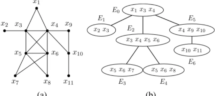
Fig. 1. A graph (a) and one possible optimal tree-decomposition (b).
methods [7], [9]–[11] use the notion of tree-decomposition [8] in order to identify independent subproblems.
Definition 2: A tree-decomposition of a graph G = (X, C) is a pair (E, T ) with T = (I, F ) a tree (I is the set of nodes and F the set of edges of T ) and E = {Ei: i∈ I} a family of subsets of X, such that each subset (called cluster) Ei is a node of T and satisfies: (i) ∪i∈IEi= X, (ii) for each edge {x, y} ∈ C, there exists i ∈ I with {x, y} ⊆ Ei, and (iii) for all i, j, ! ∈ I, if ! is on a path from i to j in T , then Ei∩ Ej ⊆ E!. The width of a tree-decomposition (E, T ) is equal to maxi∈I|Ei|−1. The tree-width w of G is the minimal width over all the tree-decompositions of G.
Figure 1 represents a graph and a possible tree-decomposition of width 3 (since the largest cluster has 4 vertices).
BTD-like algorithms [7], [10], [11] exploit a tree-decomposition rooted in a given cluster (we denote Erthe root cluster of the decomposition) which permits to decompose the original problem into many subproblems (one subproblem per cluster). Given a WCSP instance (X, D, W ), the subproblem related to the cluster Ei corresponds to the descent of Ei in the considered tree-decomposition (E, T ). More precisely, its variable set Desc(Ei)is the union of the clusters Ejbelonging to the subtree of T rooted in Ei (Ei included) while its cost functions are ones whose scope is included in Desc(Ei)but not in the separator of Eiwith its parent cluster Ep(i)(i.e. the intersection Ei∩ Ep(i), under the assumption that Ep(r)=∅). As these subproblems rooted in Ei are also related to the current assignment Aion the separator Ei∩ Ep(i), we denote them Pi|Ai. For the root cluster, the subproblem Pr|∅ rooted in Er corresponds to the initial problem.
These algorithms solve the initial problem by assigning the variables in such a way that the variables of a cluster Ei are always assigned before ones of its child clusters. By so doing, they can benefit from the independence between the subproblems induced by the used tree-decomposition. Notably, they exploit a lower bound and an upper bound per subproblem Pi|Aiwhose recording often leads to a more powerful pruning and many redundancy saving. These algorithms may rely on DFS (BTD-DFS [7], [11]) or HBFS (BTD-HBFS [7]). To this end, from a theoretical viewpoint, the advantage of using such methods can be justified by the time complexity which is gen-erally in O(n.e.dw++1
) (with w+ the width of the exploited
tree-decomposition and d the size of the largest domain) whereas classical methods have a complexity in O(n.e.dn). These methods have a space complexity in O(n.s.ds)where s is the size of the largest intersection between two clusters in the considered tree-decomposition. In the same time, from a practical viewpoint, BTD-like algorithms maintaining local consistencies make it possible to obtain very efficient methods outperforming classical methods, notably when the instances have nice structural properties [7], [11]. Of course, this effi-ciency depends on the used decompositions. Minimizing w+
can be interesting from a theoretical viewpoint. However, in practice, two elements are often considered as crucial:
• controlling the value of s since this value is directly related to the amount of memory used during the solving. Using a tree-decomposition with a large value of s may lead the method to run out of memory.
• exploiting a relevant variable ordering. It is well known that the best variable ordering heuristics (e.g. [12], [13]) require a certain freedom in the choice of the next vari-able, what may be in contradiction with the restrictions imposed on the variable ordering by the use of a tree-decomposition.
We address these two points in Sections III and IV.
III. COMPUTING TREE-DECOMPOSITIONS
Computing an optimal decomposition (i.e. a tree-decomposition having a minimum width) is well known to be a NP-hard problem [14]. Hence, computing tree-decompositions is usually achieved by heuristic methods. In this context, the heuristic Min-Fill [15] is considered as the reference method by the CP community. Thanks to its use, tree-decompositions have been already exploited successfully for solving WCSP instances [7]. Nevertheless, they have not shown their full potential because of the quality of the computed decompo-sitions. In fact, Min-Fill aims to minimize the width of the computed tree-decompositions. However, nothing guarantees that the obtained tree-decomposition is suitable for an efficient solving of WCSP instances. Notably, Min-Fill tends to produce decompositions whose clusters have few proper variables (i.e. variables belonging to a cluster but not to its parent) and whose largest separators have frequently a size close to w+.
As evoked above, such a large value of s may be problematic due to the amount of memory required for storing the local bounds for each subproblem Pi|Ai. Hence, in [7], Allouche et al. address this problem by considering a variant of Min-Fill denoted Min-Fillr4. Min-Fillr4 computes a tree-decomposition
as Min-Fill does and then each cluster sharing more than 4 variables with its parent is merged with it. By so doing, BTD-like algorithm may exploit larger clusters (which may increase the freedom of the variable heuristic) while consuming a reasonable amount of memory.
Here, we address this question in a different way. More precisely, we consider a general framework, called H-TD-WT (for Heuristic Tree-Decomposition Without Triangulation), which has been recently introduced in [16]. Unlike Min-Fill, this framework aims to produce decompositions without
computing a triangulation of the constraint graph. However, it exploits some topological features (via the connected com-ponents) and the construction of each cluster is guided by a heuristic depending on the criteria we want to fulfill. Its time complexity is reasonable, generally in O(n(n + e)) whereas, in practice, it is often faster than Fill (or Min-Fillr4). Different parameterizations are conceivable in order to
produce tree-decompositions suitable for an efficient solving. For example, these last years, three possible parameterizations of H-TD-WT have been proposed in the frame of the decision problem CSP:
• H2[17] which guarantees that the clusters of the
decom-position are connected,
• H3 [16] which identifies independent parts of the graph
and separates them as soon as possible by doing a breadth-first search.
• H5 [18] which aims to compute tree-decompositions
having separators of bounded size, with S as an upper bound on the size of the separators.
These heuristics have shown their practical interest for solving CSP instances [16], [18], [19], but have never been considered for the treatment of WCSP instances. Beyond, once the decomposition computed, it can be exploited statically like in [7], [10], [11] or dynamically as described in the next section.
IV. DYNAMIC EXPLOITATION OF THE DECOMPOSITION
BTD-like methods have shown their practical interest when solving WCSP instances having nice topological features [7], [11]. Nonetheless, they may turn to be inefficient if the instance has no particular topological feature. One possible reason is related to the variable orderings they consider. These orderings have a freedom restricted by the use of the tree-decomposition since all the variables of a given cluster must be assigned before ones of their child clusters. In particu-lar, these restrictions may prevent from taking benefits from adaptive techniques [12], [13] which, nowadays, contribute significantly to the practical efficiency of classical Branch and Bound methods. In this section, our goal is to exploit cleverly the tree-decomposition by avoiding using it systematically. More precisely, in the same spirit as adaptive techniques, whose choices rely both on the current state of the search and its previous ones, we add to BTD-like algorithms the ability to choose to exploit globally, partially or not the tree-decomposition depending on whether its exploitation seems to be beneficial or not. By so doing, we increase the freedom of the variable ordering while adapting the solving depending on the context and the nature of the instance.
In practice, the decomposition initially computed will never be exploited for a subproblem unless the solving without a decomposition seems to be inefficient. We consider, for example, the decomposition shown in Figure 2(a) represented by the set of clusters E = {Ei, Ej, Ek, El, Em, En}. Let Ei be the current cluster and A the current assignment on Ej∩Ei. We are interested by the subproblem Pj|A rooted in Ej and induced by the assignment A of the separator Ej ∩ Ei with
Ei Ej En Ek El E m Ei E! j Ei Ej En E! k (a) (b) (c)
Fig. 2. The set of the clusters of the decomposition: initial (a) when Ej is
merged with its descent (cluster E!
j) (b) when Ejis exploited (c).
Ei the parent cluster of Ej. The solving of the subproblem Pj|A does not necessarily use the decomposition, that is to say the set of the clusters {Ej, Ek, El, Em, En}. In fact, in the beginning, the solving is based on the cluster E#
jresulting from the merging of the cluster Ej with its descendants Ek, El, Em and En. Merging a cluster with its descendants consists in putting together all the variables of the descent of Ej (see Figure 2(b)). Hence, E#
j contains all the variables of the descent of Ej. Concerning the variable ordering heuristic, it benefits from a total freedom with respect to the choice of the next variable among the variables of the descent of Ej. At this level, there are two possible cases:
• The subproblem Pj|A can be easily solved when using E#
j. In this case, the exploitation of the decomposition does not seem useful.
• The solving of Pj|A is on the contrary inefficient. In this case, the exploitation of the decomposition seems wise. The cluster Ej is then re-used and the same reasoning is repeated for the cluster Ek which will be first considered as merged with its descent resulting in the cluster E#
k as shown in Figure 2(c).
Note that the reasoning is repeated for every new assignment of Ei ∩ Ej. This choice is motivated by the fact that the assignment A of the separator Ei∩ Ej induces a different subproblem from the one induced by an assignment A#. Note also that, at the level of the root cluster Er, the algorithm behaves like a classical Branch and Bound algorithm having total freedom with regard to the choice of the next variable among all the variables of the problem. Finally, the initial decomposition is fully exploited (all its clusters are exploited) when at all the levels, our algorithm decides to exploit the cluster itself rather than its descent.
For sake of simplicity, we describe now the new algorithm by exploiting DFS for solving clusters, resulting in the al-gorithm BTD-DFS+DYN (see Alal-gorithm 1). Of course, we can also derive BTD-HBFS+DYN (which will be used for the experiments) in the same manner as Allouche et al. produce BTD-HBFS from BTD-DFS [7].
Like BTD-DFS, BTD-DFS+DYN is based on a tree-decomposition (E, T ) which is computed before the solving and rooted in a cluster Er. It takes as parameters the current assignment A, the current cluster Ei, the set V of unassigned
Algorithm 1: BTD-DFS+DYN (A, Ei, V, Vdesc, clb, cub)
Input: The current assignment A, the current cluster Ei, the lower
bound clb
Input/output: The set V of unassigned variables of Ei, the set Vdesc
of unassigned variables of Desc(Ei), the current upper
bound cub
1 if Merge(Ei)then V!← Vdesc
2 else V!← V 3 if V’ "= ∅ then
4 x← pop(V!) /* Choose a variable of V!*/
5 Update V and Vdesc
6 a← pop(Dx) /* Choose a value */
7 Maintain local consistency on subproblem Pi|A ∪ {(x = a)}
8 clb!← max(clb, lb(Pi|A ∪ {(x = a)}))
9 if clb!< cubthen cub ← BTD-DFS+DYN(A ∪ {(x = a)}, Ei,
V, Vdesc, clb!, cub)
10 if max(clb, lb(Pi|A)) < cub then
11 Maintain local consistency on subproblem Pi|A ∪ {(x "= a)}
12 clb!← max(clb, lb(Pi|A ∪ {(x "= a)}))
13 if clb!< cubthen cub ← BTD-DFS+DYN
(A ∪ {(x "= a)}, Ei, V, Vdesc, clb!, cub)
14 else if ¬Merge(Ei)then
15 /* Solve all child clusters with unknown optimum */
16 S← Children(Ei)
17 while S "= ∅ and lb(Pi|A) < cub do
18 Ej← pop(S) /* Choose a child cluster */
19 if LBPj|A< U BPj|Athen
20 cub!← min (UBP
j|A, cub− [lb(Pi|A) −lb(Pj|A)])
21 cub!!← BTD-DFS+DYN (A, Ej, Ej\(Ei∩ Ej),
Desc(Ej)\(Ei∩ Ej), lb(Pj|A), cub!)
22 Update LBPf|Aand UBPf|Ausing cub!!
23 cub← min(cub, wi
∅+
!
Ej∈Children(Ei)
U BPj|A)
24 else cub ← min(cub, !
Ej⊆Desc(Ei)
w∅j)
25 return cub
variables of Ei, the set Vdesc of unassigned variables of the descent Desc(Ei)of Ei, the current lower bound clb and the current upper bound cub. It aims to compute the optimum of the problem rooted in Ei and induced by the assignment A. There are two possible cases:
• If the returned value of cub is strictly less than the input value of cub, then cub is the optimum of the subproblem. • Otherwise, cub defines a lower bound on the optimum. The initial call is BTD-DFS+DYN(∅, Er, Vr, Vrdesc, lb(Pr|∅),
k) with Vrdesc the set of variables of the descent of Er,
lb(Pr|∅) the initial lower bound obtained by exploiting a local consistency on the initial problem and k the maximal cost. Note that throughout the algorithm, wi
∅ denotes the cluster-localized lower bound for the cluster Ei. Like BTD-DFS, BTD-DFS+DYN assumes that the input problem is consistent according to the exploited local consistency and returns its optimum. Lines 3-13 of BTD-DFS+DYN aim to assign the variables of V# as BTD-DFS does for the variables of V . A pair (variable, value), (x, a), is selected according to the variable and value ordering heuristics. Given that binary branching is exploited, this choice results in either assigning the variable x to a (left branch, positive decision, line 7), or removing the value a from the domain of x (right
branch, negative decision, line 11). For each branch, local consistency is maintained on the subproblem rooted in Ei and induced by the current assignment so that a lower bound lb is computed. If the maximum clb# of the lower bound lb, deduced via the application of the local consistency, and the current lower bound clb, is strictly less than cub, the search continues; otherwise, the corresponding subtree is pruned. Lines 15-23 of BTD-DFS+DYN solve the subproblems rooted in each child cluster Ej of Ei, similarly to BTD-DFS. The subproblem Pj|A is explored unless its optimum is already known. Anyway, BTD-DFS and BTD-DFS+DYN record, for each subproblem Pj|A, two values denoted by LBPj|A and
U BPj|A. They represent respectively the best known lower and
upper bounds for Pj|A. If LBPj|A = U BPj|A, the optimum
of Pj is already computed. The recursive call corresponding to the child cluster Ej (line 21) exploits an initial non-trivial upper bound computed at line 20, as explained in [11]. It is followed by an update of both LBPj|A and UBPj|A with
the value of cub## (line 22). The exploitation of all the child clusters ends finally by updating cub.
Now that the similarities between DFS and BTD-DFS+DYN are recalled, we describe the modifications made to BTD-DFS. The function Merge represents the heuristic responsible for choosing whether the cluster Ei is exploited or its descent E#
i. The call to Merge with the cluster Ei as an input returns true if and only if E#
i is exploited. Otherwise, the cluster Ei is exploited and the freedom of the next variable choice is limited to the variables of V . One of the two parameters V or Vdesc is effectively used depending on whether Ei or Ei# is exploited. The choice between V and Vdesc is done on lines 1-2 and is memorized in V#. Both are suitably updated on line 5. If V# =∅ and E
iis not merged with its descent, BTD-DFS+DYN behaves like BTD-DFS (lines 3-13). If V# = ∅ and E
i is merged with its descent, BTD-DFS+DYN has no more variables to be assigned given that all the variables of the descent of Ei have been already assigned. In this case, BTD-DFS+DYN updates cub (line 24) at the basis of the local lower bound wj
∅ of each cluster Ej belonging to Desc(Ei). If V# (= ∅ (lines 3-13), BTD-DFS+DYN behaves the same way whether Ei or its descent Ei# is exploited, by trying to assign the variables of V#.
The algorithm BTD-DFS+DYN can be parameterized by the heuristic Merge which decides when to stop exploiting the cluster E#
iand to exploit instead the current cluster Ei(we propose one heuristic in the next section). Certainly, the choice of a relevant heuristic is essential to improve the solving.
The dynamic exploitation of the decomposition changes both the time and the space complexity. In fact, the behavior of BTD-DFS+DYN can constantly evolve. It first acts like almost a classical DFS and then, if it decides at each level to exploit the original cluster instead of its descent, it finally acts like a standard BTD-DFS.
Theorem 1: The time complexity of BTD-DFS+DYN ranges from O(exp(w++1)) to O(exp(n)) with w+ the width of
the tree-decomposition computed before the solving. Its space complexity is in O(n.s#.ds!
exploited separator of the decomposition (s# ≤ s). V. EXPERIMENTS
In this section, we assess the practical interest of the framework H-TD-WT for solving WCSP instances and we evaluate the relevancy of exploiting dynamic decompositions. But first, we describe the used experimental protocol. A. Experimental protocol
We consider the solving algorithms HBFS and BTD-HBFS(+DYN) with tree-decompositions produced by Min-Fill and Min-Fillr4. Note that, until now, HBFS and BTD-HBFS
with Min-Fillr4 are considered as the reference algorithms for
solving WCSP instances respectively without and with the exploitation of the structure [7], while Min-Fill is often used as the reference method for computing tree-decompositions by the CP community. Concerning H-TD-WT, we exploit the heuristic H2, which guarantees the connectivity of the
clusters, H3, which computes decompositions having many
child clusters and H5which controls the size of the separators.
The heuristic H5is available in two variants, denoted by H525
and H5%
5 . For H525, the size of the separators is bounded
by 25. Regarding H5%
5 , the limit of the maximum size of
separators depends on the instance and is fixed to 5% of the number of variables of the instance, normalized to a minimum upper bound of 4 (S = 4) and a maximal upper bound of 50 (S = 50).
Like [7], we exploit the implementations of HBFS, BTD-HBFS, Min-Fill and Min-Fillr4 provided in the open-source
WCSP solver Toulbar21. In order to guarantee a fair
compar-ison, we have also implemented BTD-HBFS+DYN in Toul-bar2. The Hidecompositions are computed by our own library and transmitted to Toulbar2 by means of a file.
The dynamic exploitation of the decomposition is based on a heuristic (F) that is responsible for deciding to exploit the cluster Eior its descent Ei#. The heuristic F uses the feedback given by BTD-HBFS. In fact, each call to BTD-HBFS on a subproblem Pi|A takes as input both the known lower and upper bounds, clb and cub. If within the allowed number of backtracks, BTD-HBFS does not succeed in improving any bounds, F considers that the solving of Pi|A is not progressing and increments a counter related to it. We start henceforth exploiting Ei instead of Ei#, when the counter corresponding to Pi|A attains a given limit. In the reported results, we have exploited the value 5 for this limit. This value seems to lead to the best trade-off between BTD-HBFS and HBFS among the extensive experiments we performed.
Regarding the configuration of Toulbar2, a preprocess-ing step is performed by enforcpreprocess-ing VAC (for Virtual Arc-Consistency [20]) and applying the MSD (for Min Sum Diffusion) algorithm with 1,000 iterations. Then, EDAC (for Existential Directional Arc-Consistency [21] is enforced, at each node, during the solving. The variable ordering includes both weighted-degree [12] and last conflict [22]. Regarding
1Available at https://mulcyber.toulouse.inra.fr/projects/toulbar2/
the algorithms based on BTD, the chosen root cluster is the largest cluster (for Min-Fill) or the cluster which maximizes the ratio of the number of constraints of the cluster to its size (for the other decompositions). For the solving algorithms based on HBFS, the other parameters (e.g. α, β or N) are set with the same values as in [7]. The experiments were performed on blade servers running Linux Ubuntu 14.04 each with two Intel Xeon processors E5-2609 v2 2.4 GHz and 32 GB of memory. We use the benchmark instances available at http://genoweb.toulouse.inra.fr/∼degivry/evalgm. It includes more than 3,000 instances containing stochastic graphical models from the UAI evaluation 2008 and 2010, instances from the MiniZinc Challenge 2012 and 2013 and instances from the Probabilistic Inference Challenge 2011. Compared to [7], we have discarded instances solved during the pre-processing, resulting in a benchmark of 2,444 instances. For each instance, the solving is performed with a timeout of 20 minutes (including when applicable, the computation of the decomposition) and 16 GB of memory.
Before giving in details the experimental results, it seems necessary to give additional comments on the comparisons between the respective runtimes of the different approaches. Indeed, one method could be considered as more efficient if its runtime is better. However, we must also take into account the number of solved instances. For example, when we report in Figures 3 (a) and (b) that BTD-HBFS using Min-Fill solves 1,712 instances in 26,291 s, while BTD-HBFS+DYN using H25
5 solves 2,039 instances in 52,304 s, we can be interested
by the bench solved by at least one of both methods which involves 2,049 instances. We can see that BTD-HBFS using Min-Fill have solved only 1,712 instances among the 2,049 instances while consuming 430,691 seconds. Here, we add the cost of the 337 unsolved instances in 20 minutes, that is 404,400 seconds which must be added to the 26,291 s used to solve the 1,712 instances. Concerning BTD-HBFS+DYN using H25
5 , after adding the cost of the 10 instances unsolved
among the 2,049 instances, we obtain a total of 64,304 s. By this way, we see that finally, BTD-HBFS+DYN (using H25
5 )
runs 6 times faster than BTD-HBFS (using Min-Fill) while it solves 327 additional instances.
B. H-TD-WT vs. Min-Fill / Min-Fillr4
In this part, we compare the behavior of BTD-HBFS de-pending on the different exploited decompositions. Regarding the computation of decompositions, we notice that the compu-tation of Hidecompositions (with i ∈ {2, 3, 5}) is much faster than Min-Fill. More precisely, any Hi is able to decompose 2,431 instances in less than 1,200 s whereas Min-Fill requires 19,044 s to decompose 2,415 instances.
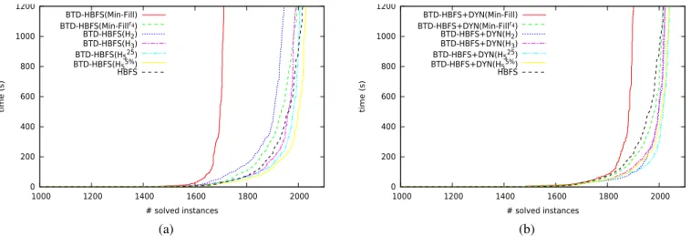
Figure 3(a) shows the cumulative number of solved in-stances w.r.t. the runtime for HBFS and BTD-HBFS with Min-Fill and the decompositions computed thanks to H-TD-WT. First, we note that Min-Fill solves the weakest number of instances within 20 minutes (only 1,712 instances). It shows that, despite the difficulty of the WCSP problem, the heuristics that aim only to minimize the size of clusters are not the
0 200 400 600 800 1000 1200 1000 1200 1400 1600 1800 2000 time (s) # solved instances BTD-HBFS(Min-Fill) BTD-HBFS(Min-Fillr4) BTD-HBFS(H2) BTD-HBFS(H3) BTD-HBFS(H525) BTD-HBFS(H55%) HBFS 0 200 400 600 800 1000 1200 1000 1200 1400 1600 1800 2000 time (s) # solved instances BTD-HBFS+DYN(Min-Fill) BTD-HBFS+DYN(Min-Fillr4) BTD-HBFS+DYN(H2) BTD-HBFS+DYN(H3) BTD-HBFS+DYN(H525) BTD-HBFS+DYN(H55%) HBFS (a) (b)
Fig. 3. Cumulative number of solved instances w.r.t. the runtime in seconds for HBFS and BTD-HBFS (a) or BTD-HBFS+DYN (b) depending on the decompositions.
more efficient. In fact, in order to minimize the width of the produced tree-decomposition, Min-Fill tends to produce clusters which have few proper variables. So the variable ordering heuristic is almost useless and the exploited variable ordering is nearly static. The results also show that the others parameters have more impact on the solving than the width of the decomposition, like the connectivity of the clusters (H2),
the number of child clusters (H3) or the size of the separators
(Min-Fillr4and H
5). Limiting the size of the separators seems
to increase significantly the efficiency of the solving. In fact, if BTD-HBFS with H2and H3 solves respectively 1,945 and
1,989 instances, the decompositions having bounded separa-tors size lead to solve more than 2,000 instances. However, comparing Min-Fillr4 to H
5shows that BTD-HBFS associated
to H5 permits to solve more instances especially with H55%,
which allows to solve 2,029 instances against 2,000 instances solved by BTD-HBFS with Min-Fillr4. Furthermore,
BTD-HBFS exploiting Min-Fillr4 requires 98,861 s to solve these
instances whereas BTD-HBFS exploiting H5%
5 requires only
58,792 s. Finally, note that these results are consistent with those obtained for the decision problem CSP in [16]. C. Dynamic decomposition assessment
We evaluate now BTD-HBFS+DYN. Both Figures 3 (a) and (b) show that, regardless of the exploited decomposi-tion, HBFS+DYN solves more instances than BTD-HBFS. The increase of the number of solved instances can be remarkable like in the case of Min-Fill that permits to solve now 1,905 instances instead of 1,712 instances. The exploitation of H2 and H3 with BTD-HBFS+DYN allows to
solve 2,023 instances against respectively 1,945 and 1 989 solved by BTD-HBFS. The exploitation of Min-Fillr4 and
H5 with BTD-HBFS+DYN is also improved with regard to
their utilization with BTD-HBFS. In particular, H25
5 allows
to solve 2,039 instances, which constitutes the largest number of solved instances among all the possible combinations of a solving algorithm and a decomposition we consider. Beyond
1 10 100 1000 1 10 100 1000 BTD-HBFS +DYN ( H 5 25 ) BTD-HBFS+DYN ( Min-Fillr4 )
Fig. 4. Runtime comparison of BTD-HBFS+DYN with H25
5 and Min-Fillr4. the increase in the number of solved instances, the cumulative runtime decreases. For instance, BTD-HBFS+DYN requires 74,159 s for solving 2,019 instances with Min-Fillr4 (resp.
52,304 s for 2,039 instances with H25
5 ), while BTD-HBFS
solves 2,000 instances in 98,861 s (resp. 2,006 instances in 56,553 s).
We now focus on comparing H25
5 and Min-Fillr4with
HBFS+DYN. Figures 3(b) and 4 show clearly that BTD-HBFS+DYN is globally more efficient with H25
5 than with
Min-Fillr4. This trend still holds when we consider the
bench-mark of instances solved by both BTD-HBFS+DYN with Min-Fillr4and BTD-HBFS+DYN with H25
5 , in order to fairly
com-pare their respective runtime. Indeed, this benchmark includes 2,013 instances solved by BTD-HBFS+DYN with Min-Fillr4 in 71,249 s against only 41,372 s by BTD-HBFS+DYN with H25
0.001 0.01 0.1 1 10 100 1000 0.001 0.01 0.1 1 10 100 1000 BTD-HBFS+DYN ( H 5 25 ) BTD-HBFS ( Min-Fillr4) 1 10 100 1000 1 10 100 1000 BTD-HBFS +DYN ( H 5 25 ) HBFS (a) (b)
Fig. 5. (a) Runtime comparison between BTD-HBFS+DYN with H25
5 and BTD-HBFS with Min-Fillr4 (a) and HBFS (b).
D. BTD-HBFS(+DYN) vs. the best known methods
At now, BTD-HBFS with Min-Fillr4 and HBFS are
con-sidered as the best known methods for solving WCSPs re-spectively with and without exploiting the structure. So, it is quite natural to compare them to BTD-HBFS(+DYN) with H5.
Figures 3(a), 3(b) and 5(a) clearly show that BTD-HBFS and
BTD-HBFS+DYN with H5%
5 or H525outperform significantly
BTD-HBFS with Min-Fillr4, w.r.t. both the number of solved
instances and the cumulative runtime. For instance,
BTD-HBFS+DYN with H25
5 solves 2,039 instances in 52,304 s
while BTD-HBFS with Min-Fillr4 requires 98,861 s to solve
2,000 instances.
We now compare BTD-HBFS(+DYN) with H5 to HBFS.
First we can note that BTD-HBFS with H5%
5 is more efficient
than HBFS. Notably, it solves more instances than HBFS, namely 2,029 instances against 2,017 instances by HBFS and, in addition, it has a better cumulative runtime with 58,792 s against 84,555 s for HBFS. This can be essentially explained by the recordings achieved by BTD-HBFS via the separators, that is to say a lower bound and an upper bound on the optimum of the corresponding subproblem. Furthermore, BTD-HBFS distinguishes independent subproblems, which is not the case of HBFS.
Then a similar trend can be observed if we compare
BTD-HBFS+DYN associated to H25
5 to HBFS (see Figure 5(b)).
Indeed, BTD-HBFS+DYN with H25
5 turns to solve more
instances and faster than HBFS. Moreover, if we consider the 2,008 instances solved by both algorithms, HBFS solves them in 79,020 s against only 43,914 s for BTD-HBFS+DYN with H525.
We now focus our comparison to the hardest instances. More precisely, we discard easy instances, which are even trivial sometimes (that is to say instances being solved in less than 10 s by HBFS). Note that these instances are also easily solved by BTD-HBFS+DYN provided that at the level of the root cluster BTD-HBFS+DYN behaves as HBFS (when the descent of the root cluster is exploited). Among the 794
remaining instances, at least one leaf cluster of the decom-position is exploited for 279 instances. In other words, there exists at least one branch of the decomposition that is entirely exploited (in the sense of the set of the clusters of the original decomposition). For 423 instances, the decomposition is never exploited which means that BTD-HBFS+DYN behaves as HBFS. Regarding the remaining instances, the decomposi-tion is exploited till a particular depth without reaching a leaf cluster of the decomposition. Hence, in practice, BTD-HBFS+DYN can simply behave like HBFS or progressively decide to exploit the original clusters of the decomposition (instead of their descent) until reaching the behavior of BTD-HBFS.
Finally, we compare the lower and the upper bounds reported by HBFS and BTD-HBFS+DYN when a timeout occurs. Among the 375 instances not solved neither by HBFS nor by BTD-HBFS+DYN, for 252 instances, the upper bound computed by BTD-HBFS+DYN is strictly less than the one computed by HBFS against only 52 instances for HBFS. Also, for 229 instances, BTD-HBFS+DYN reports a higher lower bound than HBFS against 146 instances for HBFS. Figure 6 compares the gap between the lower and the upper bounds for both algorithms. Clearly, BTD-HBFS+DYN offers a reduced gap compared to HBFS. This shows that even when the instance is not solved, BTD-HBFS+DYN is able to give approximations of better quality than HBFS.
E. Summary
All of these results show that exploiting a decomposition dynamically seems to enhance the efficiency of the solving by enabling BTD-HBFS+DYN to adapt the solving to the nature of the instance and by avoiding using a decomposition when solving a problem (or a subproblem) without a decomposition is more efficient. It results than BTD-HBFS+DYN with H25
5 is
able to outperform the best known methods for solving WCSPs like BTD-HBFS with Min-Fillr4 or HBFS w.r.t. the number
1 100 10000 1e+06 1e+08 1e+10 1e+12
1 100 10000 1e+06 1e+08 1e+10 1e+12
BTD-HBFS+DYN ( H
5
25 )
HBFS
Fig. 6. Gap between the lower and the upper bounds for both BTD-HBFS+DYN with H25
5 and HBFS.
VI. CONCLUSION
The tree-decompositions have been already exploited with success to solve WCSP instances. At the same time, their potential was not fully revealed especially due to the quality of the used decompositions. In fact, like Min-Fill, the computed decompositions usually aim to minimize the size of the clusters (in order to minimize the theoretical time complexity bound) to the detriment of the practical efficiency of the solving. So, in order to take into account other relevant parameters (i.e. having additional impact on the solving efficiency w.r.t. the width), we have first exploited the framework H-TD-WT, which has been previously proposed to solve CSP instances. This framework aims to compute decompositions much faster than by classical heuristics. It also permits to take into consideration relevant properties with respect to the solving efficiency such as the maximal size of separators with the H5 heuristic. Utilizing
H5 with BTD-HBFS has clearly proven the interest of
H-TD-WT. Indeed, H5 does not only improve the performance
of BTD-HBFS compared to BTD-HBFS exploiting Min-Fill, but has permitted to outperform significantly HBFS. On the other hand, we have proposed an extension of BTD-HBFS, called BTD-HBFS+DYN, which exploits the decomposition dynamically. The idea consists in using the decomposition only for a subproblem whose solving without decomposition seems to be inefficient. It notably avoids to restrict unnec-essarily the freedom of the variable ordering heuristic for “easy” subproblems. In practice, we have shown that BTD-HBFS+DYN improves BTD-HBFS, regardless of the exploited decomposition, with regard to both the number of solved instances and the cumulative runtime. Consequently, thanks to this extension, structural methods are henceforth highlighted versus non-structural methods.
Several extensions of this work seem relevant. For example, the computation of the decomposition made before the solving can also be achieved dynamically. In fact, the decomposition is often partially used, not to mention the case where the decomposition is not exploited at all by BTD-HBFS+DYN.
Moreover, it would also make it possible to calculate better and more adapted decompositions for the solving of WCSP instances than those calculated solely on the basis of struc-tural criteria. Beyond that, other heuristics for the dynamic exploitation of decompositions may be assessed.
ACKNOWLEDGMENT
This work has been funded by the french Agence nationale de la Recherche, reference ANR-16-C40-0028.
REFERENCES
[1] C. Cabon, S. de Givry, L. Lobjois, T. Schiex, and J. P. Warners, “Radio Link Frequency Assignment,” Constraints, vol. 4, pp. 79–89, 1999. [2] M. Sanchez, S. de Givry, and T. Schiex., “Mendelian error detection in
complex pedigrees using weighted constraint satisfaction techniques,” Constraints, vol. 13, no. 1-2, pp. 130–154, 2008.
[3] M. Cooper and T. Schiex, “Arc consistency for soft constraints,” Artificial Intelligence, vol. 154(1-2), pp. 199–227, 2004.
[4] S. de Givry, F. Heras, J. Larrosa, and M. Zytnicki, “Existential arc consistency: closer to full arc consistency in weighted CSPs,” in IJCAI, 2005.
[5] M. C. Cooper, S. de Givry, and T. Schiex, “Optimal Soft Arc Consis-tency,” in IJCAI, 2007, pp. 68–73.
[6] M. Cooper, S. Givry, M. Sanchez, T. Schiex, M. Zytnicki, and T. Werner, “Soft arc consistency revisited,” Artificial Intelligence, vol. 174, pp. 449– 478, 2010.
[7] D. Allouche, S. de Givry, G. Katsirelos, T. Schiex, and M. Zytnicki, “Anytime hybrid best-first search with tree decomposition for weighted CSP,” in CP, 2015, pp. 12–29.
[8] N. Robertson and P. Seymour, “Graph minors II: Algorithmic aspects of treewidth,” Algorithms, vol. 7, pp. 309–322, 1986.
[9] A. Koster, “Frequency Assignment - Models and Algorithms,” Ph.D. dissertation, University of Maastricht, Novembre 1999.
[10] C. Terrioux and P. J´egou, “Bounded backtracking for the valued con-straint satisfaction problems,” in CP, 2003, pp. 709–723.
[11] S. de Givry, T. Schiex, and G. Verfaillie, “Exploiting Tree Decomposi-tion and Soft Local Consistency in Weighted CSP,” in AAAI, 2006, pp. 22–27.
[12] F. Boussemart, F. Hemery, C. Lecoutre, and L. Sais, “Boosting system-atic search by weighting constraints,” in ECAI, 2004, pp. 146–150. [13] P. Refalo, “Impact-based search strategies for constraint programming,”
in CP, 2004, pp. 557–571.
[14] S. Arnborg, D. Corneil, and A. Proskuroswki, “Complexity of finding embeddings in a k-tree,” SIAM Journal of Disc. Math., vol. 8, pp. 277– 284, 1987.
[15] D. J. Rose, “Triangulated Graphs and the Elimination Process,” Journal of Mathematical Analysis and Application, vol. 32, pp. 597–609, 1970. [16] P. J´egou, H. Kanso, and C. Terrioux, “An Algorithmic Framework for
Decomposing Constraint Networks,” in ICTAI, 2015, pp. 1–8. [17] P. J´egou and C. Terrioux, “Combining Restarts, Nogoods and
Decom-positions for Solving CSPs,” in ECAI, 2014, pp. 465–470.
[18] P. J´egou, H. Kanso, and C. Terrioux, “Towards a Dynamic Decompo-sition of CSPs with Separators of Bounded Size.” in CP, 2016, pp. 298–315.
[19] P. J´egou and C. Terrioux, “Tree-decompositions with connected clusters for solving constraint networks,” in CP, 2014, pp. 407–423.
[20] M. C. Cooper, S. de Givry, M. S´anchez, T. Schiex, and M. Zytnicki, “Virtual arc consistency for weighted csp,” in AAAI, 2008, pp. 253–258. [21] S. de Givry, F. Heras, M. Zytnicki, and J. Larrosa, “Existential arc consistency: Getting closer to full arc consistency in weighted csps,” in IJCAI, 2005, pp. 84–89.
[22] C. Lecoutre, L. Sa¨ıs, S. Tabary, and V. Vidal, “Reasoning from last conflict (s) in constraint programming,” Artificial Intelligence, vol. 173, no. 18, pp. 1592–1614, 2009.