Contents lists available atScienceDirect
Robotics and Autonomous Systems
journal homepage:www.elsevier.com/locate/robotMonitoring a robot swarm using a data-driven fault detection
approach
Belkacem Khaldi
a,
Fouzi Harrou
b,*
,
Foudil Cherif
a,
Ying Sun
baLESIA Laboratory, Department of Computer Science, University of Mohamed Khider, R.P. 07000 Biskra, Algeria
bKing Abdullah University of Science and Technology (KAUST), Computer, Electrical and Mathematical Sciences and Engineering (CEMSE) Division, Thuwal 23955-6900, Saudi Arabia
h i g h l i g h t s
• Two new approaches to fault detection in robotic swarm systems are developed. • Combining advantages of univariate PCA and SPC charts.
• Virtual viscoelastic control model is used for the circle formation of the robot swarm. • The simulation results show effectiveness of the proposed approaches.
a r t i c l e i n f o Article history:
Received 3 February 2017
Received in revised form 1 May 2017 Accepted 6 June 2017
Available online 30 June 2017
Keywords:
Exogenous fault detection Swarm robotics Viscoelastic control model Data-driven approaches Statistical monitoring schemes
a b s t r a c t
Using swarm robotics system, with one or more faulty robots, to accomplish specific tasks may lead to degradation in performances complying with the target requirements. In such circumstances, robot swarms require continuous monitoring to detect abnormal events and to sustain normal operations. In this paper, an innovative exogenous fault detection method for monitoring robots swarm is presented. The method merges the flexibility of principal component analysis (PCA) models and the greater sensitivity of the exponentially-weighted moving average (EWMA) and cumulative sum (CUSUM) control charts to insidious changes. The method is tested and evaluated on a swarm of simulated foot-bot robots performing a circle formation task, via the viscoelastic control model. We illustrate through simulated data collected from the ARGoS simulator that a significant improvement in fault detection can be obtained by using the proposed method where compared to the conventional PCA-based methods (i.e., T2and Q ).
©2017 Elsevier B.V. All rights reserved.
1. Introduction
1.1. The state of the art
Swarm intelligence techniques in multi-robotics systems are among the fast growing areas in the field of robotics [1–3]. The philosophy behind the swarm robotics field is inspired by the societies of animals such as birds, ants and bees. Indeed, the lim-ited capability of a single robot to perform complex tasks can be enhanced by using a robotic swarm [4,5]. Furthermore, a group of robots, which is able to cooperate to perform complex tasks is important in process industries to enhance productivity, efficiency, and safety, and to increase the flexibility of the whole swarm system. Moreover, swarm robotics is very useful for several ap-plications, such as the collective detection of bombs, cooperative search and exploration, managing warehouses, delivering products
*
Corresponding author. Fax: +966 12802 1386.E-mail address:[email protected](F. Harrou).
to customers, the seeding, harvesting, and storing of grains, and rescuing human beings in emergency situations.
In practice, assigned tasks are not always expected to be prop-erly executed at the desired performance level when using a robotic swarm system. This is mainly due to external interferences or failures resulting from component faults such as bugs in a robot’s software controller, electromechanical faults in a robot’s sensors and actuation devices, or from topological faults like bro-ken communication links and intrusions between robots of the swarm. Of course, one or more faulty robots can lead to degraded performance of the swarm and failure to comply with the target requirements. Therefore, it is crucial to detect and identify possible faults or failures in the monitored robotic swarm system as early as possible. Accurate and prompt fault detection efficiency and operating capacity of the swarm system, and expense maintenance is avoided.
Generally, faults in robot swarms are difficult to avoid and may result in serious system degradations [6]. Monitoring in swarm robotics has lately received special attention from researchers and
http://dx.doi.org/10.1016/j.robot.2017.06.002
practitioners in the field of safety engineering. Increased atten-tion to fault detecatten-tion and safety has led to the development of several fault detection techniques that can be grouped into two main families [7,8]: endogenous and exogenous fault detection techniques. Endogenous approaches are used to monitor each robot individually to reveal any faults. Several works report using such an approach; Skoundrianos et al. used a local model neural network to diagnose faults in the wheels of a mobile robot [9]. Yuan et al. [10] proposed a hybrid fault diagnosis approach based on Mittag-Leffler kernel (ML-kernel) support vector machine (SVM) and Dempster–Shafer fusion for wheeled robot driving system. Christensen et al. [11,12] proposed a time-delay neural networks for automatic synthesis task-dependent fault detection modules in s-bot robots. Canham et al. [13] implemented an immune-based error detection method which takes inspiration from the negative selection process of the immune system on both a Khepra robot and a BAE system RascalTM robot. Mokhtar et al. [14] adapted a fault detection algorithm (called modified Dendritic Cell Algorithm mDCA) loosely inspired by the functioning of dendritic cells in the immune system. However, such approaches ignore the interaction between robots and therefore may result in a misleading diagnosis. For example, a robot might not detect anomalies in itself, such as a dead battery or a software bug, and it cannot even signal the rest of the swarm if an anomaly occurs in its communications hardware. In addition, these methods use only the data collected from, ignoring the data available in the whole swarm, which may result in the loss of pertinent information [7].
On the other hand, exogenous fault detection techniques were developed to inspect several robots simultaneously [15]. In other words, a robot could detect errors that arise in another robot’s components by taking into consideration the available information of its neighborhood in the swarm [15]. Owens et al. [16], and Jaki-movski et al. [17] proposed an AIS-based fault detection algorithm inspired by the T-Cell Receptor and intracellular signaling network mechanisms to detect anomalies within autonomous swarm sys-tems. Christensen et al. [6] proposed a firefly-inspired exogenous fault detection approach to detect inoperative robots in the swarm. Tarapore et al. [18] presented an AIS-based exogenous approach to detect faults in robotic swarm systems and tested its performance on different case studies that included aggregating, dispersing, flocking, and harming. Khadidos et al. [19] presented a model-based exogenous fault detection method model-based on broadcasting the sensor readings and motor speeds of robots to their neighbors. Millard et al. [20] proposed a run-time fault detection approach using an internal prediction model in each robot to compare with the real behavior of other robots in the swarm.
Both endogenous and exogenous techniques can be developed using either a mathematical model or an empirical implicit model for fault detection. In mathematical model-based approaches, faults are detected based on a comparison between the actual behaviors of the monitored system with predicted behaviors de-rived from a mathematical model of the system. Unfortunately, deriving accurate models of monitored systems, especially com-plex industrial process systems that include robot swarms, can be difficult and time consuming. Data-driven implicit models are a suitable alternative in the absence of an explicit model, and if measurement signals are the only available resource for process monitoring. Unlike the mathematical model-based approaches, data-based techniques efficiently extract useful features for the design of monitoring schemes, based on empirical models derived from the available process data. Such methods require minimal prior knowledge about process physics, but depends on the avail-ability of quality input data. Indeed, data-driven methods are mainly based on computational intelligence and machine learning methods. Multivariate statistical process control (MSPC) charts are one of the tools that have been used to reach these objectives.
1.2. Motivation and contributions
While several fault detection techniques have been proposed for robotic swarm systems, MSPC charts have not been used for monitoring in swarm robotics until recently. This paper focus on monitoring robot swarms using PCA-based fault detection ap-proaches. Principal component analysis (PCA) is a basic method of multivariate analysis and is a powerful tool for monitoring multivariate processes with highly correlated process data. PCA is one the most commonly used techniques for dimension reduction. Using the PCA method, the covariance structure in data can be explained in a reduced dimensional space through an orthogonal set of principal components (PCs), i.e, a set of linear combina-tions of the original variables. Faults in the monitored swarm can be detected by extracting useful data from the original dataset through PCA modeling, and then monitoring against those indices. However, conventional PCA-based monitoring indices such as T2
and Q charts lose the ability to detect small changes in the mean of process data [21,22].
The overarching goal of this paper is to tackle multivariate chal-lenges in process monitoring by merging the advantages of tradi-tional univariate and multivariate techniques to enhance their per-formance and widen their practical applicability. Exponentially-weighted moving average (EWMA) and cumulative sum (CUSUM) control charts are widely used univariate control charts. The key idea is to apply PCA dimension reduction techniques to the fea-tures of a process, and use control charts to monitor only the more informative variables, or principal components. Specifically, we extend the abilities of the univariate monitoring techniques such as EWMA and CUSUM to deal with multivariate processes by developing linear PCA-based EWMA and CUSUM monitoring methods to monitor robotic swarm systems. Note that the main advantage of the PCA-based EWMA and CUSUM fault detection approaches is that the testing step is performed online, which is not the case in a classifier (the classifier algorithms are performed offline rather than online). A decision can be made for each new sample by comparing the value of the EWMA or CUSUM decision statistic with the value of the threshold. An anomaly is declared if the EWMA or CUSUM statistic exceeds the threshold. The proposed monitoring approach is applied to detect faults in a swarm of foot-bot rofoot-bots while they are forming a circle. We refer to the virtual viscoelastic control (VVC) model proposed in [23] for robot swarm circle formation; this model was previously implemented on sim-ulated e-puck robots using the ARGoS simulator [24]. Here we implement the model again on simulated foot-bot robots. During the simulation, we collect various inputs and outputs of data for each robot of the swarm; these data are later used in the PCA model for monitoring.
The following section briefly reviews the VVC model used for the robot swarm’s circle formation. Section3review the PCA-based approach and how it can merged with the EWMA and CUSUM charts for fault detection. In Section5, the performances of the pro-posed methods are illustrated in a simulation study, and Section6 concludes with a discussion and suggestions for future research directions.
2. Virtual viscoelastic control model
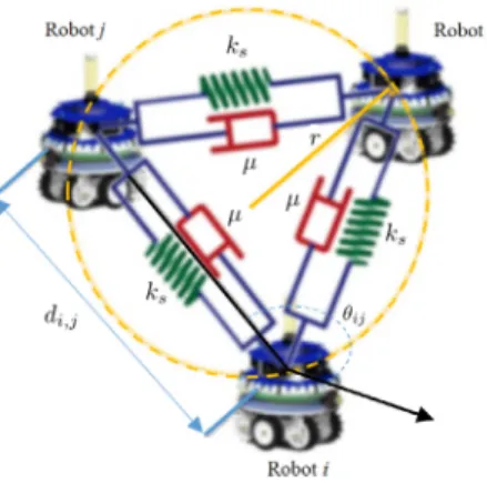
The virtual viscoelastic control (VVC) model is a physics-based model that has been successfully applied as a proximal control to keep and arrange robots together within a certain distance [23,25]. In this model, the movement of the swarm is governed by virtual viscoelastic forces, which result from the interactions of the robots with each other. This allows connectivity and coherency between the robots of the swarm while they are in motion.Fig. 1illustrates a model setup of three foot-bot robots forming a circle with radius
Fig. 1. A circle formation of three robots using the viscoelastic control (VVC) model.
r via the VVC model. The motion of each robot (its right speed
v
r i and left speedv
li) depends on the virtual viscoelastic force Fivvc, which is given by the following equation:Fvvc i
=
nX
j=1 fvvc ij,
(1) fvvc ij=
(ks(di,j d0)+ µv
i,j),
(2)where d0
=
2r sin(⇡ /
(n+
1)), n is the number of neighbors, ksis the spring constant, di,jis the displacement vector that represents the current length of the spring between two interacting robots, d0isthe equilibrium length of the spring,
µ
is the damping coefficient,and
v
i,jis the velocity of the focal robot relative to its nearby mate. The speeds of the robot’s wheels are computed as follows:
v
liv
ri=
2
6
4
1 b 2 1 b 23
7
5
v
i!
i.
(3)Here b is the distance between the robot’s wheels. The robot’s angular velocity
!
iand the robot’s forward speedv
i are given as follows:!
i=
k! 6 Fivvc, v
i=
p
v
max| !
i| +
1 (4)where k!is a gain constant,6 Fvvc
i refers to the angle formed by the force Fvvc
i , and
v
maxis the maximum allowed forward speed. To achieve the VVC model in a foot-bot robot, we use its range and bearing device (RAB). With this device, the foot-bot is able to send and receive messages to and from nearby robots within a maximum range Dr. Moreover, it can also perceive the range (dij) and bearing (✓
ij) measurements of the robot that sent a message. Details about the values of constants and parameters we used in the model can be found in the works of Khaldi and Cherif [23,25].3. PCA-based monitoring approaches
The goal of PCA is to explain the variance/covariance structure through an orthogonal set of linear combination of original vari-ables in the reduced dimensional space. Due to dependency and collinearity, much of the variation can be accounted for by only small number of principal components (PCs).
3.1. Feature extraction using PCA
Consider a properly scaled data matrix or measurement matrix
X
=
⇥
xT1
, . . . ,
xTn⇤
T2
Rn⇥m, with n measurements and m process variables. In the following discussion, it is assumed that the scaleddata is zero-mean centered with unit variance. Usually, due to redundancy and noise in the data, l, principal components (l
⌧
m)can capture much of the variability in X. The data matrix X can be expressed by PCA as two complementary orthogonal parts: a modeled data
b
X which contains the most significant variationspresent in the data and a residual data E which represents noises, i.e., X
=
TPT=
X
l i=1 tipTi+
mX
i=l+1 tipTi= b
X+
E,
(5) where T= [
t1 t2· · ·
tm] 2
Rn⇥m represents a matrix of the transformed uncorrelated variables, ti2
Rn termed principal components (PCs), which are defined as uncorrelated, linear com-binations of the original variables that successively maximize the total variance of data projection. l is the number of PCs retained in the PCA model. The column vectors pi2
Rm, termed the loading vectors, arranged in the matrix P2
Rm⇥mare obtained by the eigenvectors related to the covariance matrix of X, i.e., ⌃. Theloading vectors are the eigenvectors of the covariance matrix,⌃.
Through singular value decomposition,⌃can be decomposed as: ⌃
=
1n 1XTX
=
P⇤PT with PPT=
PTP=
In.
(6) Here,⇤=
diag( 12, . . . ,
m2) is a diagonal matrix containing theeigenvalues of⌃in decreasing magnitude, and Inis the identity matrix [26]. In PCA, it is very important to select the optimal number of PCs to be retained in the model [27]. There are many techniques for selecting the dimension l, such as cross-validation, cumulative percent variance (CPV), and variance of reconstruction error. In this paper, the CPV technique is employed to determine the number of retained PCs, l: CPV (l)
=
PPli=1 im
i=1 i
⇥
100.3.2. PCA-based fault detection
Once a PCA model based on past normal operation is obtained, it can be used to monitor future deviation from normality. Two monitoring statistics, the T2and Q statistics, are usually utilized for
fault detection purposes [28]. The T2statistic based on the number
of retained PCs, l, is defined as [28]: T2
=
X
l i=1 t2 i i,
(7)where iis eigenvalue of the covariance matrix of X. The T2statistic measures the variation in the PCs only. A large change in the PC subspace is observed if some points exceed the confidence limit of the T2chart, indicating a big deviation in the monitored
system. Confidence limits for T2at level (1
↵
) relate to the Fisherdistribution, F, as follows [28]:
T2
l,n,↵
=
l(n 1)
n l Fl,n l,↵
,
(8)where Fl,n l,↵is the upper 100
↵
% critical point of F with l and n l degrees of freedom.The squared prediction error (SPE) or Q statistic, which is de-fined as [28]:
Q
=
eTe,
(9)captures the changes in the residual subspace. e
=
x x representsˆ
the residuals vector, which is the difference between the new ob-servation, x, and its prediction,x, via PCA model. Eq.
ˆ
(9)provides a direct mean of the Q statistic in terms of the total sum of measured variation in the residual vector e. The SPE can be considered a measure of the system-model mismatch. The confidence limitsfor SPE are given by [26]. This test suggests the existence of an abnormal condition when Q
>
Q↵, where Q↵, is defined as:Q↵
= '
1
h 0c↵p
2'
2'
1+
1+
'
2h0(h0 1)'
12,
(10)where c↵is the confidence limits for the 1
↵
percentile in a normaldistribution,
'
i=
P
mj=l+1 ij,
for i=
1,
2,
3, and h0=
1 2'31''23 2 .However, the PCA-based T2 and Q approaches fail to detect
small faults [29]. The CUSUM and EWMA charts, which are widely used univariate control charts, are proposed as improved alterna-tives for fault detection. The objective is to tackle PCA challenges in process monitoring by merging the advantages of the CUSUM, EWMA, and PCA approaches to enhance their performance and widen their practical applicability.
4. Univariate statistical control charts
Univariate statistical methods, such as CUSUM and EWMA, have been widely used to monitor industrial processes for many years. These methods are briefly reviewed here.
4.1. EWMA monitoring charts
EWMA is a statistic which gives less weight to old data, and more weight to new data. The EWMA charts are able to detect small shifts in the process mean, since the EWMA statistic is a time-weighted average of all previous observations. The EWMA monitoring chart is an anomaly-detection technique widely used by scientists and engineers in various disciplines [30–35]. Assume that
{
x1,
x2, . . . ,
xn}
are individual observations collected from a monitored process. The expression for the EWMA is [35]:zt
=
xt+
1 zt 1 if t>
0.
(11)The starting value z0 is usually set to the mean of the
fault-free data,
µ
0. zt is the output of EWMA and xt is the observation from the monitored process at the current time. The forgetting parameter2
(0,
1]
determines how fast EWMA forgets historicaldata. We can see that if is small, then more weight is assigned to past observations. Thus the chart is tuned to have efficiency for detecting small changes in the process mean. On the other hand, if is large, then more weight is assigned to the current observations, and the chart is more suitable for detecting large shifts [34,35]. As approaches zero, EWMA approximates the CUSUM criteria, which gives equal weights to the current and historical observations.
The upper and lower control limits of the EWMA chart for detecting a mean shift are: UCL
/
LCL= µ
0±
L zt, whereL is a multiplier of the EWMA standard deviation zt, zt
=
0
q
(2 )
[
1 (1 )2t]
, and 0 is the standard deviation of thefault-free or preliminary dataset. The parameters L and need to be set carefully [34,35]. In practice, L is usually set to 3, which corresponds to a false alarm rate of 0.27%. If ztis within the interval [LCL UCL], then we conclude that the process is under control up to time point t. Otherwise, the process is considered out of control.
4.2. Cumulative sum (CUSUM) charts
Like the EWMA chart, CUSUM charts have also a good capacity to detect small shifts in the process mean due to an extensive memory of the process [36]. The CUSUM chart aggregates all the information from past and current samples in the decision proce-dure. The CUSUM statistic (Si) is defined as the following [35]:
St
=
nX
j=1
(xj
µ
0),
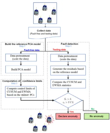
(12)Fig. 2. A flowchart of a PCA-based fault detection schemes.
0 500 1000 Time step 0 50 100 0 500 1000 2 4 8 6
Fig. 3. Evolution in time of (a) AMDE, and (b) GS.
where t denotes the current time point, St is the cumulative sum of all samples, including the most recent, and
µ
0is the targetedprocess mean. A one-sided CUSUM statistic is computed using the following equation [35]: St
=
tX
j=1
xj (µ
0+
k),
(13)where k is a parameter used as a reference to detect changes in the process mean. If Stbecomes negative, then the CUSUM statistic is set to zero. An out-of-control process is defined by St exceeding the decision interval, which is another parameter needed for the CUSUM charts to function. The parameters k and h are defined as k
=
2, and h=
d2, respectively, where d
=
22 ln 1↵ ,=
x, xis the standard deviation of the average of the process variable (x) being monitored,↵
and are probabilities, and is thesize of the shift in the mean that needs to be detected. In practice, Montgomery recommends using a value of 4 or 5 for h [35]. This choice would provide a reasonable detection for a shift of 1 in the
Table 1
PCA-based EWMA and CUSUM fault detection procedures.
Step Action
1. Given:
•A training fault-free dataset that represents the normal process operations and a testing dataset (possibly faulty data),
•The parameters of the EWMA control scheme: smoothing parameter and the control limit width L, 2. Data preprocessing
•Scale the data to zero mean and unit variance, 3. Build the PCA model using the training fault-free data
•Express the data matrix as a sum of approximate and residual matrices as shown in Eq.(5), •Compute the ignored principal components using PCA.
•Compute the control limits of the EWMA and CUSUM control schemes 4. Test the new data
•Scale the new data,
•Compute the ignored principal components using the builded PCA model, •Compute the EWMA and CUSUM decision statistics,
5. Check for faults
•Declare a fault when the EWMA or CUSUM decision function exceeds the control limits previously computed using the training data.
process mean. Numerous variations of the CUSUM exist; for more details see [35].
4.3. Combining PCA with CUSUM and EWMA charts
Once a PCA model based on historical, normal data is obtained, it can be utilized to monitor future deviation of the process. In this paper, we combine the advantages of PCA modeling with those of the univariate monitoring charts, CUSUM and EWMA, which results in an improved fault detection system, especially for detecting small faults in highly correlated, multivariate data. Towards this end, we applied CUSUM and EWMA charts to the ‘‘minor’’ components obtained from PCA model. As we know, the principal components (PCs) explain most of the variation in the data; minor components refer to the unimportant or residual infor-mation that is not retained in a PCA model. The minor components, which capture the variability that arises from noise, represent the residuals of the process, and may contain redundancies that exist between variables. Thus, the loading vectors related to the minor components actually describe the correlations between variables. Indeed, under normal operation with little noise and few errors, the minor components are close to zero, while they significantly deviate from zero in the presence of abnormal events. In this work, the minor components are used as fault indicator. Few studies have taken the minor components into account when doing PCA analysis.
The implementation of the developed monitoring methods is comprised of two stages: offline modeling and online monitoring. In the offline modeling phase, PCA is performed on the normal operating data (training data) enabling us to obtain a reference model. Then, the fault detection procedure is executed by using the reference PCA model with EWMA and CUSUM charts in the online monitoring phase. The PCA-based CUSUM and EWMA fault detection algorithms are schematically summarized as shown in Table 1, which is schematically represented inFig. 2.
The methodology of using PCA for statistical process monitoring is illustrated through a simulated robot swarm in the next section.
5. Results and discussion
In this study, we perform ARGoS-based experimental simu-lations on a swarm of foot-bots; the robots are programmed to perform the VVC model to self-organize into a uniform circle from a randomly dispersed distribution. ARGoS comes with a configu-ration file in which we can set the arena, the robots, their sensors, and their actuators devices. In our simulation setup, we activate the RAB equipment within a range Dr
=
3 m, the arena is set to a closed room of 10⇤
6 m2, the number of the foot-bots is setTable 2
Data collected from the ARGoS simulation.
Parameter Description
AMDE Average mean distance error [25]
GS Group speed [25]
vri Right wheel forward speed
vli Left wheel forward speed
Fvvc
i Virtual viscoelastic force length
6 Fvvc
i Virtual viscoelastic angle
to n
=
6, the foot-bots are randomly distributed in the arena, and their orientations are set to be a Gaussian distribution of zero means and a standard deviation of 360 . In ARGoS, the simulation time step is set to 0.1 s, with five iterations each experiment, for a total of 1500 time steps. During the experimental simulations, we collect data that are further used as inputs and outputs for the PCA-based monitoring approach; we summarize these data inTable 2. Fig. 3plots the average of the five running simulations for both the group speed, GS, and the average mean distance error, AMDE, of the entire swarm. The plots show that from time step t=
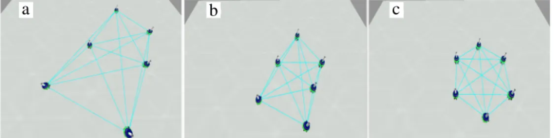
500, the robotic swarm system becomes stable and converges to a constantAMDE and a tiny variable GS.Fig. 4shows ARGoS-based snapshots in step times (t
=
0,
t=
250, and t=
500) during the VVC modelsimulation with a swarm of six foot-bots.
5.1. PCA modeling
In this study, a swarm of six robots is considered. The data matrix X used to build a PCA model contains 3000 observations and 12 variables (i.e., viscoelastic force length and viscoelastic force angle collected from each robot). These twelve signals measured when the swarm system is operating normally. Moreover, all the measured observations are collected during the stabilization phase of the swarm system (from starting point of a time window (t
=
500) to the end of the simulation). First, these training data are scaled to zero mean and variance one, then used to build the PCA model. The number of PCs retained in the PCA model are determined using the CPV method with a threshold of 95%. The first PC explains 56% of the total variance; the second PC explains 37% of the total variance, and the third PC explains 3% of the total variance. Together, three PCs can capture 96% of the useful information in the monitored robotic swarm system (seeFig. 5). Thus, only three PCs need to be retained in the PCA model.
Monitoring results of the PCA-based T2, Q , and EWMA charts for
the normal operating data are shown inFig. 6(a–c). Since the Q plot shown inFig. 6(b) is based on normal operating data, one should expect that almost all the data will lie within the 95% confidence
b
a
c
Fig. 4. Snapshots during ARGoS simulation of 6 foot-bots performing the VVC model at: (a) t=0, (b) t=250 and (c) t=500.
Fig. 5. Three PCs capture 96% of information in the system.
interval. Similarly, the data points in the PCA–EWMA and CUSUM charts are also within the 95% confidence limits (seeFig. 6(c–d)). However, the T2plot given inFig. 6(a) shows a few false alarms.
We can conclude that the PCA model describes the data well when no faults are presents.
5.2. Detection results
After a system model has been successfully identified, we can proceed with fault detection. Five types of faults in robotic swarm systems will be considered here: abrupt, intermittent, random walk, complete stop, and gradual faults.
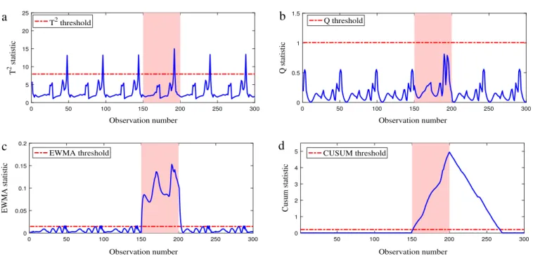
5.2.1. Case (A): Abrupt fault detection
In this case study, an abrupt change is simulated by adding a small, constant deviation to the viscoelastic force length of the first robot, x1, between sample times 150 and 200. Since the viscoelastic
force is largely related to the RAB device, this could represent a misperception of the range of neighbors or noisy data (velocities) received from neighbors. The two examples below show the per-formance of the fault detection techniques in detecting an abrupt fault.
Case (A1): In the first example, the magnitude of the deviation
is equal to 40% of the total variation in x1. Monitoring results are
shown inFig. 7(a–d). The T2chart, as expected, has no ability to
whatsoever to detect this moderate fault (seeFig. 7(a)). This fact is due to the PCs subspace sometimes being insensitive to moderate and small faults, because each PC is a combination of all process variables. The monitoring results of the PCA-Q , PCA–EWMA, and PCA–CUSUM charts are demonstrated inFig. 7(b–d). All the charts show signs of a fault because the bias shift in this case is quite large.
Case (A2): In the second example, a bias fault of 10% of the
total variation is introduced in x1between sample times 150 and
200. This could represent a total sensor offset or noisy sensing in the RAB device; this means a possible misperception of both the range and the bearing measurements of neighbors, in addition to possible miscommunications received from neighbors. The four monitoring charts are shown inFig. 8(a–d). The T2and Q charts
are demonstrated inFig. 8(a–b), from which we can see that they cannot give any sign of an anomaly. The major reason for this over-sight of the conventional PCA-based monitoring methods (i.e., T2
and Q ) is that they use current observation data alone to evaluate system performance ignoring the historical data. We then apply the CUSUM chart with k
=
0.
25 and h=
0.
19 and the EWMA chartwith
=
0.
3 to the testing dataset. Both statistics clearly exceedthe control limits, indicating the occurrence of some abnormal condition. However, the CUSUM chart gave several false alarms, an error rate of 26.4%. Indeed, after conditions return to normal, the CUSUM chart continues to show abnormality for some time, resulting in a large number of false alarms. This case study clearly shows the superiority of the EWMA chart over all other charts.
5.2.2. Case (B): Intermittent fault
In this case study, we introduce into the testing data a bias of amplitude 40% of the total variation in x1of between samples 50
and 100, and a bias of 10% between samples 150 to 200. This again could be due to a repeated misperception of the range and the bearing measurements for nearby robots or noisy received data (a RAB sensor fault).Fig. 9(a–d) shows the monitoring results of the PCA-based T2, Q , EWMA, and CUSUM charts.Fig. 9(a) shows
that the PCA-based T2 chart has no power to detect this fault.
FromFig. 9(b), it can be seen that the PCA-Q chart can detect the intermittent faults but with several missed detections. It can be seen fromFig. 9(d) that the PCA–CUSUM chart can indeed detect this fault, but with some missed detections. On the other hand, the PCA–EWMA chart with
=
0.
3 correctly detects this intermittentfault (seeFig. 7(c)). In this case study, we can see that detection performance is much enhanced when using the PCA–EWMA chart compared to the others.
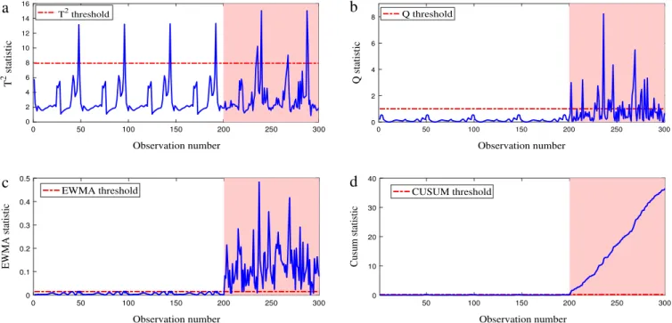
5.2.3. Case (C): Random walk fault
As the movement pattern of swarming robots is highly cross-correlated, we investigate the ability of the proposed approaches to detect a random walk fault in a robot swarm. In this case study, the first robot is performing a random walk and not following the other robots. Such an event could occur when there are noises in the RAB device of the robot. To generate the data with a random
0 0.5 1 1.5 0.25 0.2 0.15 0.1 0 0.05 0.02 0.015 0.01 0 0.005
Fig. 6. Monitoring results of PCA-T2(a), PCA-Q (b), and PCA–EWMA charts (c) for the normal operation data.
25 20 15 10 0 5
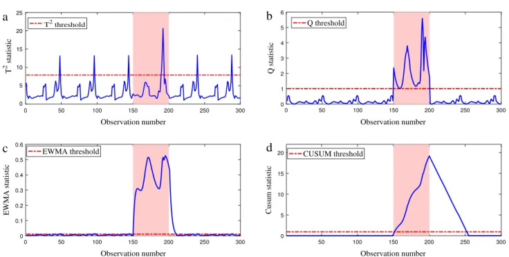
Fig. 7. Monitoring results of the T2(a), Q (b), EWMA with =0.3 (d), and CUSUM (with k=0.25 and h=0.19) (c) charts in the presence of an abrupt fault in x 1from
sample 150 to 200 (Case (A1)).
walk fault, the viscoelastic force length of the first robot, x1, is
contaminated with random Gaussian noise with a variance of
=
0
.
5 from sample number 200 until the end of the test data. Thefour monitoring charts are shown inFig. 10(a–d). The PCA-T2chart
fails to detect this fault, as shown inFig. 10(a).Fig. 10(a) shows that the PCA-Q is able to detect the fault, but with several missed detections. On the other hand, the PCA-based CUSUM and EWMA charts perform reasonably well (seeFig. 10).
5.2.4. Case (D): Complete stop fault
In this case study, the detection of a complete stop fault in a robot swarm is investigated. In this case study, we consider a complete stop error, which is when a robot has completely stopped working, becoming invisible to neighboring robots. For this pur-pose, the value of the viscoelastic force of the first robot is zeroed
from sampling time 200 until the end of the test data. This means that both the RAB device and the motor actuator of the faulty robot have completely stopped working (the robot can move nor send or receive messages). Here the T2chart can detect the fault but with
several missed detections (seeFig. 11). The other three charts, PCA-based Q , CUSUM, and EWMA, all perform reasonably well because the anomaly in this case is relatively large.
To quantify the efficiency of the proposed strategies, we use two metrics: the false detection rate (FAR) and the miss detection rate (MDR) [37]. The FAR is the number of normal observations that are wrongly judged as faulty (false alarms) over the total number of fault-free data. The MDR is the number of faults that are wrongly classified as normal (missed detections) over the total number of faults. The FDR and MDR of the above examples are summarized in Table 3. The smaller the FAR and MDR are, the better the detection
Fig. 8. Monitoring results of the T2(a), Q (b), EWMA with =0.3 (d), and CUSUM (with k=0.25 and h=0.19) (c) charts in the presence of an abrupt fault in x 1from
sample 150 to 200 (Case (A2).
Fig. 9. Monitoring results of the T2(a), Q (b), EWMA with =0.3 (d), and CUSUM (with k=0.25 and h=0.19) (c) charts in the presence of intermittent faults in x 1
between sample times [50 100] and [150 200] (Case (B)). Table 3
False and miss detection rates for all monitoring charts.
Chart Case (A1) Case (A2) Case (B) Case (C) Case (D)
FAR MDR FAR MDR FAR MDR FAR MDR FAR MDR
T2 2 92 2 98 2 93 2 94 2 66
Q 0 0 0 100 0 44 0 74 0 0
CUSUM 20 2 26.4 2 75 0 0 2 0 0
EWMA 7.6 0 4 0 5.5 0 3.5 5 0 0
rate is. FromTable 3it can be seen that the developed PCA–EWMA chart provides better detection performances compared to the other charts when detecting small and persistent faults.
5.2.5. Case (E): Drift failure detection
A ramp type, or slow drift, fault is simulated by adding a ramp change to the normal measurements of x1 from sample
Fig. 10. Monitoring results of the T2(a), Q (b), EWMA with =0.3 (d), and CUSUM (with k=0.25 and H=0.19) (c) charts when the first robot performs a random walk
from sample number 200 through the end of the testing data, Case (C).
Fig. 11. Monitoring results of the T2(a), Q (b), EWMA with =0.3 (d), and CUSUM (with k=0.25 and h=0.19) (c) charts when the first robot has completely stopped
working between sample times 200–300, Case (D).
150 through the end of the testing data. This means that either a gradual decrease of the viscoelastic force has occurred due to degradation of a battery, or a sudden increase of robot speed has happened due to problems in the robot’s motor.Fig. 12(a) shows that the PCA-T2 is not sensitive to this drift fault. The PCA-Q
chart is shown inFig. 12(b), which first flags the fault at sample 181.Fig. 12(c) shows that the PCA–EWMA chart first detects the fault at the 157th observation. Therefore, fewer observations are needed for the PCA–EWMA chart to detect a fault compared to the other charts. This case study testifies again to the superiority of the proposed approaches compared to conventional PCA-based
fault detection. Of course, this paper also demonstrates through simulated data that significant improvement in fault detection can be obtained by using the PCA model when combined with well established statistical techniques such as the EWMA and CUSUM charts.
6. Conclusion
This paper focuses on an improved data-based fault detection strategy and its application to fault detection in a swarm of foot-bot rofoot-bots. Towards this end, the VVC model is used for the circle
Fig. 12. Monitoring results of the T2(a), Q (b), EWMA with =0.3 (d), and CUSUM (with k=0.25 and h=0.19) (c) charts in the presence of a drift fault with slope 0.01
in x1from sample 150, Case (E).
formation of the robot swarm. Different kind of faults have been tested in this study including abrupt faults, drift faults, random walks and complete stop faults. The swarm data, simulated via the ARGoS simulator, show that significant improvement in fault detection can be obtained by using the EWMA chart instead of the Q or T2 charts, which are conventionally used with
PCA-based techniques. Because the PCA-PCA-based T2and Q charts evaluate
monitored system performance based on the current data alone, they are suitable for detecting relatively large faults. They are less capable of detecting relatively small and persistent shifts, compared to the CUSUM and EWMA charts.
Conventional PCA models are most suitable for dealing with a steady state system. However, in practice systems are usually dynamic and time-varied. Directly applying the PCA method to monitor or model such a process often results in false alarms and model-process mismatch. To adapt to a process drift or change of operating point, we plan in future work to develop a recursive model by updating an online PCA model.
In future works, experimental data will be used to test and validate the performance of the proposed approach in detecting faults in a robot swarm. Experimental data could be recorded using external tracking systems, or via using on-board sensors. An ex-ternal tracking system is generally an exex-ternal infrastructure, with the required sensors, that should be installed to record the needed measurements. For example, the Vicon tracking system [38] built at Bristol Robotics Lab (BRL) implements virtual sensors, to allow online evolution of collective behaviors within a swarm of e-puck robots. The OptiTrack system [20] installed at the York Robotics Lab (YRL) provides high precision real-time position tracking, to perform a comparison between the expected and the observed be-havior in an e-puck robot augmented with a Linux Extension Board (LEB). However due the height cost of such tracking infrastructures, an alternative approach to be used in our future works is the use of the robot on-board sensors such as the range and bearing (RAB) equipment [39]. The RAB can be used to broadcast the observed data (i,e Fvvc
i and6 Fivvc) computed by each foot-bot robot to one or more robots that act as observers. The observer(s) will then perform the PCA-based fault detection approach, to independently monitor the behavior of the other robots that are within their range of perception.
Acknowledgments
This publication is based upon work supported by the King Abdullah University of Science and Technology (KAUST) Office of Sponsored Research (OSR) under Award No: OSR-2015-CRG4-2582. The work is done in collaboration with the LESIA Laboratory, Department of Computer Science, University of Mohamed Khider, Biskra, Algeria. We would like to thank the reviewers of this article for their insightful comments, which helped us to greatly improve its quality.
References
[1] M. Senanayake, I. Senthooran, J.C. Barca, H. Chung, J. Kamruzzaman, M. Murshed, Search and tracking algorithms for swarms of robots: A survey, Robot. Auton. Syst. 75 (2016) 422–434.
[2] B. Khaldi, F. Cherif, An overview of swarm robotics: Swarm intelligence applied to multi-robotics, Int. J. Comput. Appl. 126 (2) (2015).
[3] Y. Tan, Z. Zheng, Research advance in swarm robotics, Defence Technol. 9 (1) (2013) 18–39.
[4] B. Yang, Y. Ding, Y. Jin, K. Hao, Self-organized swarm robot for target search and trapping inspired by bacterial chemotaxis, Robot. Auton. Syst. 72 (2015) 83–92.
[5] P. Levi, E. Meister, F. Schlachter, Reconfigurable swarm robots produce self-assembling and self-repairing organisms, Robot. Auton. Syst. 62 (10) (2014) 1371–1376.
[6] A. Christensen, R. O’Grady, M. Dorigo, From fireflies to fault-tolerant swarms of robots, IEEE Trans. Evol. Comput. 13 (4) (2009) 754–766.
[7] A. Millard, J. Timmis, A. Winfield, Towards exogenous fault detection in swarm robotic systems, in: Conference Towards Autonomous Robotic Sys-tems, Springer, 2013, pp. 429–430.
[8] H. Lau, Error detection in swarm robotics: A focus on adaptivity to dynamic environments, 2012.
[9] E. Skoundrianos, S. Tzafestas, Finding fault-fault diagnosis on the wheels of a mobile robot using local model neural networks, IEEE Robot. Autom. Mag. 11 (3) (2004) 83–90.
[10] X. Yuan, M. Song, F. Zhou, Z. Chen, Y. Li, A novel Mittag-Leffler kernel based hybrid fault diagnosis method for wheeled robot driving system, Comput. Intell. Neurosci. 2015 (2015) 65.
[11] A. Christensen, R. O ´Grady, M. Birattari, M. Dorigo, Fault detection in au-tonomous robots based on fault injection and learning, Auton. Robots 24 (1) (2008) 49–67.
[12] A. Christensen, R. O’Grady, M. Birattari, M.M. Dorigo, Automatic synthesis of fault detection modules for mobile robots, in: AHS, 2007, pp. 693–700.
[13]R. Canham, A. Jackson, A. Tyrrell, Robot error detection using an artificial im-mune system, in: NASA/DoD Conference on Evolvable Hardware, IEEE, 2003, pp. 199–207.
[14]M. Mokhtar, R. Bi, J. Timmis, A. Tyrrell, A modified dendritic cell algorithm for on-line error detection in robotic systems, in: IEEE Congress on Evolutionary Computation, IEEE, 2009, pp. 2055–2062.
[15]H. Lau, I. Bate, P. Cairns, J. Timmis, Adaptive data-driven error detection in swarm robotics with statistical classifiers, Robot. Auton. Syst. 59 (12) (2011) 1021–1035.
[16]N. Owens, A. Greensted, J. Timmis, A. Tyrrell, T cell receptor signalling inspired kernel density estimation and anomaly detection, in: International Conference on Artificial Immune Systems, Springer, 2009, pp. 122–135.
[17]B. Jakimovski, E. Maehle, Artificial immune system based robot anomaly detection engine for fault tolerant robots, in: International Conference on Autonomic and Trusted Computing, Springer, 2008, pp. 177–190.
[18]D. Tarapore, P. Lima, J. Carneiro, A. Christensen, To err is robotic, to toler-ate immunological: fault detection in multirobot systems, Bioinspiration & Biomimetics 10 (1) (2015) 016014.
[19]A. Khadidos, R. Crowder, P. Chappell, Exogenous fault detection and recovery for swarm robotics, IFAC-PapersOnLine 48 (3) (2015) 2405–2410.
[20]A. Millard, J. Timmis, A. Winfield, Run-time detection of faults in autonomous mobile robots based on the comparison of simulated and real robot behaviour, in: 2014 IEEE/RSJ International Conference on Intelligent Robots and Systems, IEEE, 2014, pp. 3720–3725.
[21]F. Harrou, M. Madakyaru, Y. Sun, S. Khadraoui, Improved detection of incipient anomalies via multivariate memory monitoring charts: Application to an air flow heating system, Appl. Therm. Eng. 109 (2016) 65–74.
[22]F. Harrou, F. Kadri, S. Khadraoui, Y. Sun, Ozone measurements monitoring using data-based approach, Process Safety and Environmental Protection 100 (2016) 220–231.
[23]B. Khaldi, F. Cherif, Swarm robots circle formation via a virtual viscoelastic control model, in: 8th International Conference on Modelling, Identification and Control, ICMIC, IEEE, 2016, pp. 725–730.
[24]C. Pinciroli, V. Trianni, R. O’Grady, G. Pini, A. Brutschy, M. Brambilla, N. Mathews, E. Ferrante, G.D. Caro, F. Ducatelle, ARGoS: a modular, parallel, multi-engine simulator for multi-robot systems, Swarm Intell. 6 (4) (2012) 271–295.
[25]B. Khaldi, F. Cherif, A virtual viscoelastic based aggregation model for self-organization of swarm robots system, in: Conference Towards Autonomous Robotic Systems, Springer, 2016, pp. 202–213.
[26]J. Jackson, G. Mudholkar, Control procedures for residuals associated with principal component analysis, Technometrics 21 (1979) 341–349.
[27]M. Zhu, A. Ghodsi, Automatic dimensionality selection from the scree plot via the use of profile likelihood, Comput. Statist. Data Anal. 51 (2006) 918–930.
[28]S. Qin, Statistical process monitoring: Basics and beyond, J. Chemom. 17 (8/9) (2003) 480–502.
[29]F. Harrou, M. Nounou, H. Nounou, M. Madakyaru, PLS-based EWMA fault detection strategy for process monitoring, J. Loss Prev. Process Ind. 36 (2015) 108–119.
[30]J. Lucas, M. Saccucci, Exponentially weighted moving average control schemes: properties and enhancements, Technometrics 32 (1) (1990) 1–12.
[31]F. Harrou, M. Nounou, Monitoring linear antenna arrays using an exponentially weighted moving average-based fault detection scheme, Syst. Sci. Control Eng.: An Open Access J. 2 (1) (2014) 433–443.
[32]P. Morton, M. Whitby, M.-L. McLaws, A. Dobson, S. McElwain, D. Looke, J. Stackelroth, A. Sartor, The application of statistical process control charts to the detection and monitoring of hospital-acquired infections, J. Quality Clin. Pract. 21 (4) (2001) 112–117.
[33]F. Harrou, M. Nounou, H.N. Nounou, A statistical fault detection strategy using PCA based EWMA control schemes, in: 9th Asian Control Conference, ASCC, IEEE, 2013, pp. 1–4.
[34]F. Kadri, F. Harrou, S. Chaabane, Y. Sun, C. Tahon, Seasonal ARMA-based SPC charts for anomaly detection: Application to emergency department systems, Neurocomputing 173 (2016) 2102–2114.
[35]D.C. Montgomery, Introduction to Statistical Quality Control, John Wiley & Sons, New York, 2005.
[36]E. Page, Continuous inspection schemes, Biometrika 41 (1/2) (1954) 100–115.
[37]F. Harrou, Y. Sun, M. Madakyaru, Kullback-Leibler distance-based enhanced detection of incipient anomalies, J. Loss Prev. Process Ind. 44 (2016) 73–87.
[38]A.F. Winfield, C. Blum, W. Liu, Towards an ethical robot: internal models, con-sequences and ethical action selection, in: Conference Towards Autonomous Robotic Systems, Springer, 2014, pp. 85–96.
[39]A. Millard, Exogenous Fault Detection in Swarm Robotic Systems (Ph.D. disser-tation), University of York, 2016.
Belkacem Khaldi holds in 2012 a M.Sc. in image syn-thesis and Artificial life from the university of Biskra, Algeria. From the same university, he possessed a de-gree of engineer in Computer sciences in 2001. Actually he is preparing his Ph.D. in computer science at Biskra University under the supervision of Pr. Foudil Cherif. In parallel he is working since 2006 as a software developer at Sonatrach Company, Algeria. He is focusing his studies mainly on selforganized patterns, self-organized flock-ing and self-organized aggregation in swarm robotics; he is also interested in monitoring approaches applied to swarm robotics.
Fouzi Harrou received the Dipl.-Ing in Telecommunica-tions from Abou Bekr Belkaid University, Algeria, in 2004 and the M.Sc. degree in Telecommunications and Net-working in 2006 from the University of Paris VI, France. In 2010, he received the Ph.D. degree in Systems Opti-mization and Security from the University of Technology of Troyes (UTT), France, and was an Assistant Professor at the UTT, from 2009 to 2010. In 2010, he was an Assistant Professor at the Institute of Automotive and Transport Engineering at Nevers, France. From 2011 to 2012, he was Postdoctoral Research Associate at the Systems Modelling and Dependability Laboratory, UTT. From 2012 to 2014, he was an Assistant Re-search Scientist, in Chemical Engineering Department at the Texas A&M Univer-sity at Qatar, Doha, Qatar. Since 2015, he is Postdoctoral Fellow in the Division of Computer, Electrical and Mathematical Sciences and Engineering (CEMSE) at King Abdullah University of Science and Technology (KAUST). His current research interests include statistical decision theory and its applications, fault detection and signal processing, and Spatio-temporal statistics with environmental applications. He is a Member of the IEEE Computational Intelligence Society.
Foudil Cherif is a professor of computer science at Com-puter Science Department, Biskra University, Algeria. Pr. Cherif holds Ph.D. degree in computer science. The topic of his dissertation is behavioral animation: crowd simulation of virtual humans. He also possesses B.Sc. (engineer) in computer science from Constantine University 1985, and an M.Sc. in computer science from Bristol University, UK in 1989. He is currently the head of LESIA Laboratory. His current research interest is in Artificial intelligence, Artificial life, Crowd simulation, RFID security and web services.
Ying Sun is an Assistant Professor of Statistics in the di-vision of Computer, Electrical and Mathematical Sciences and Engineering (CEMSE) at King Abdullah University of Science and Technology (KAUST) in Saudi Arabia. She joined KAUST in June 2014 after one-year service as an assistant professor in the Department of Statistics at the Ohio State University, USA. At KAUST, she leads a mul-tidisciplinary research group on environmental statistics, dedicated to developing statistical models and methods for space–time data to solve important environmental problems. Prof. Sun received her Ph.D. degree in Statistics from Texas A&M University in 2011, and was a postdoctorate researcher in the research network of Statistics in the Atmospheric and Oceanic Sciences (STATMOS), affiliated with the University of Chicago and the Statistical and Applied Mathemat-ical Sciences Institute (SAMSI). She demonstrated excellence in research and teach-ing, published research papers in top statistical journals as well as subject matter journals, won multiple best paper awards from the American Statistical Association and the Transportation Research Board National Academies. Her research interests include spatio-temporal statistics with environmental applications, computational methods for large datasets, uncertainty quantification and visualization, functional data analysis, robust statistics, statistics of extremes.