Noise dynamics in multi-Stokes Brillouin laser

(1)

HAL Id: tel-03210055

https://tel.archives-ouvertes.fr/tel-03210055

Submitted on 27 Apr 2021

HAL is a multi-disciplinary open access archive for the deposit and dissemination of sci-entific research documents, whether they are pub-lished or not. The documents may come from teaching and research institutions in France or abroad, or from public or private research centers.

L’archive ouverte pluridisciplinaire HAL, est destinée au dépôt et à la diffusion de documents scientifiques de niveau recherche, publiés ou non, émanant des établissements d’enseignement et de recherche français ou étrangers, des laboratoires publics ou privés.

Noise dynamics in multi-Stokes Brillouin laser

Ananthu Sebastian

To cite this version:

Ananthu Sebastian. Noise dynamics in multi-Stokes Brillouin laser. Optics [physics.optics]. Université Rennes 1, 2020. English. �NNT : 2020REN1S068�. �tel-03210055�

(2)

T

HESE DE DOCTORAT DE

L'UNIVERSITE DE RENNES 1

ECOLE DOCTORALE N°596

Matière, Molécules, Matériaux Spécialité : « Photonique »

Noise dynamics in multi-Stokes Brillouin laser

Thèse présentée et soutenue à Lannion, le 18 décembre 2020 Unité de recherche : INSTITUT FOTON (UMR 6082/CNRS)

Par

Ananthu SEBASTIAN

Rapporteurs avant soutenance :

Yves JAOUEN Professeur, Telecom Paris Tech

Olivier LLOPIS Directeur de recherche CNRS, LAAS-CNRS

Composition du Jury :

Présidente : Medhi ALOUINI Professeur, Université de Rennes 1/ Institut Foton Examinateurs : Anne AMY-KLEIN Professeure, Université Sorbonne Paris Nord/ LPL

Jean-Charles BEUGNOT Chargé de recherche, Institut Femto-ST Carlos ALONSO-RAMOS Chargé de recherche CNRS, C2N

Dir. de thèse : Pascal BESNARD Professeur, ENSSAT( Université de Rennes1)/ Institut Foton

(3)

(4)

iii

Acknowledgement

I would like to extend my sincere gratitude towards the remarkable individuals who have supported and helped me throughout my PhD at Institut FOTON. It has been a time of intense learning for me, not only in the scientific field but also on a personal level.

First and foremost, I wish to thank my principal supervisor Pascal BESNARD for giving me the opportunity to pursue my PhD at the University of Rennes1, France. His excellent guidance, confidence, supervision and continuous encouragement have been a constant inspiration that made so many things possible throughout my research. Pascal always trusted me and find time to discuss during heavy administrative tasks incumbent on him. In addition, I would like to thank my co-supervisor, Stephane TREBAOL for his guidance, friendship, and extended support in the course of my research. All my supervisor’s motivation and immense knowledge always helped me during my PhD and writing this thesis.

Besides supervisors, I would like to acknowledge my jury members Yves JAOUEN and Olivier LLOPIS for accepting to be the reporter of this manuscript. Many thanks for their very relevant remarks. I thank Anne AMY-KLEIN from LPL, Jean-Charles BEUGNOT from Institut Femto-ST, Carlos ALONSO-RAMOS from C2N and Medhi ALOUINI from Institut Foton for their constructive questions during the defense.

With a special mention to Irina V Balakireva, who contributed the numerical simula-tions and theoretical model for noise analysis. I would like to acknowledge the valuable inputs from Schadrac Fresnel and Mohamed Omar Sahni, who contributed to many fruit-ful discussions and showed me all the details of experimental physics in the initial phase of my PhD, which always helped me to achieve valuable insights into Brillouin laser.

I would also like to thank all of the academic and support staff of the Institut FO-TON and ENSSAT for their fruitful discussions and assistance throughout my research period. I would also thank all my colleagues and friends, Antoine Congar, Dominique

(5)

iv

Mammez, Nessim Jebali, Joseph Slim, Georges Perin, Louis Ruel, Rasool Saleem and Amith Karuvath, who made my life simple, enjoyable and memorable at FOTON. It was a great pleasure to work with you and thank you so much for your friendship and for all the good times!

Finally, I could not conclude these thanks without having thought of my inspiring parents and sister, fantastically supportive family members, and my enchanting friends.

Thank you

(6)

v

Abstract

Stimulated Brillouin Scattering (SBS) is a coherent interaction process in which light is scattered from optically generated acoustic waves. It is a powerful tool for microwave and optical signal processing, distributed sensing and spectroscopy. Brillouin lasers are attracting a lot of interest for their ability to produce ultra coherent linewidths.

This thesis is devoted to the understanding of noise properties of Brillouin fiber ring lasers, operating with multiple Stokes orders. First, we present a technique based on the cavity ringdown method, which allows to characterize the Brillouin gain coefficient directly from probing the laser cavity. Its advantages are to obtain parameters from a single experiment with low optical powers (some 10 milliwatts) for short cavities (a few meters long, or integrated cavities).

Secondly, it is shown that an intrinsic linewidth of a few tens of mHz can be easily obtained by cascading two non-resonant Brillouin lasers (for which the pump performs a single pass inside the cavity). In order to obtain these results, the long-term stability has been improved by using a Pound-Drever-Hall servo loop, which allows us to compare our analytical and experimental results. Unfortunately, we were unable to explore the fundamental limits of noise reduction due to the noise floor of our bench.

Thirdly, one of the major works of this thesis is the theoretical and experimental study of the noise properties, including frequency noise and relative intensity noise, of a resonant Brillouin laser (for which pump and Stokes waves are resonant inside the cavity). In particular, the impacts of the fiber-ring-cavity quality factor, Brillouin gain detuning, are evaluated very precisely on the laser RIN features such as amplitude noise reduction and relaxation frequency.

We emphasize the fact that many characteristics of the frequency noise are related to the RIN properties by a coupling between intensity and phase. We show that the cascade process modifies the dynamics of the Brillouin laser when compared to those of a

(7)

vi

single-mode Brillouin laser with a single first-order Stokes component. Our experimental results are in excellent agreement with our numerical simulations, obtained thanks to our non-linear system describing the operation of a multi-Stokes Brillouin laser. This good match is mainly due to our ability:

• to obtain very precise values of the cavity parameters and the Brillouin gain coef-ficient using the CRDM technique ;

• to achieve long-term stability (hours);

• to finely control the detuning between the laser Stokes resonance and the frequency of the Brillouin gain maximum.

We demonstrate experimentally for the first time that frequency noise is degraded in the presence of anti-Stokes Brillouin scattering. We also show that a gain detuning of the order of a few hundred kHz can degrade the intensity noise reduction or also increase the linewidth by amplitude-phase coupling. All these very fine observations thus allow us to set the fundamental limits of such laser systems such as: the increase in noise due to anti-Stokes orders; the role of pump noise and its possible interrelation with cavity finesse; the effect of the detuning inherent to higher Stokes orders.

All these conclusions are key to the design and engineering of these Brillouin fiber lasers, which are currently attracting a great deal of interest as evidenced by the work in progress in the scientific community. This PhD thesis contributes to a better under-standing of multi-Stokes Brillouin lasers.

Keywords : Nonlinear optics, Stimulated Brillouin Scattering, Brillouin laser, fre-quency noise, relative intensity noise, laser linewidth, optical resonator, cavity ring down spectroscopy, frequency stabilization.

(8)

vii

Résumé

La diffusion Brillouin stimulée (SBS) est un processus d’interaction cohérent, pour lequel la lumière est diffusée à partir des ondes acoustiques générées optiquement. C’est un outil puissant pour le traitement des micro-ondes et des signaux optiques, la détection distribuée et la spectroscopie. Les lasers Brillouin suscitent un très grand intérêt pour leur capacité à produire des largeurs de raie ultra cohérentes.

Cette thèse est consacrée à la compréhension des propriétés de bruit des lasers à fibre Brillouin en anneau, fonctionnant avec de multiples ordres de Stokes. Tout d’abord, nous présentons une technique basée sur la méthode de ringdown de la cavité, qui permet de caractériser le coefficient de gain Brillouin directement à partir du sondage de la cavité laser. Ses avantages sont d’obtenir des paramètres à partir d’une seule expérience avec de faibles puissances optiques (quelques 10 milliwatts) pour des cavités courtes (quelques mètres de long, ou cavités intégrées).

Deuxièmement, il est démontré qu’une largeur de raie intrinsèque de quelques dizaines de mHz peut être facilement obtenue en cascadant deux lasers Brillouin non résonants (pour lesquels la pompe effectue un seul passage à l’intérieur de la cavité). Afin d’obtenir ces résultats, la stabilité à long terme a été améliorée en utilisant une boucle d’asservissement de type Pound Drever Hall, ce qui nous permet de comparer nos résultats analytiques et expérimentaux. Malheureusement, nous n’avons pas exploré les limites fondamentales de la réduction du bruit en raison du plancher de bruit de notre banc de mesure.

Troisièmement, un des travaux majeurs de cette thèse est l’étude analytique et ex-périmentale des propriétés du bruit, y compris le bruit de fréquence et le bruit relatif d’intensité, d’un laser Brillouin résonant (pour lequel, les ondes de pompe et de Stokes sont résonantes à l’intérieur de la cavité). En particulier, les impacts du facteur de qualité de la cavité fibrée en anneau, le désaccord de gain Brillouin ont été évalués très précisé-ment sur les caractéristiques du RIN du laser telles que la réduction de l’amplitude du

(9)

viii

bruit et la fréquence de relaxation.

Nous soulignons le fait que de nombreuses caractéristiques du bruit de fréquence sont liées aux propriétés du RIN par un couplage entre l’intensité et la phase. Nous montrons que le processus en cascade modifie la dynamique du laser Brillouin par rapport à celle d’un laser Brillouin monomode avec une seule composante de Stokes de premier ordre. Nos résultats expérimentaux sont en excellent accord avec nos simulations, obtenues grâce à notre système non linéaire décrivant le fonctionnement d’un laser Brillouin multi-Stokes. Cette bonne concordance est principalement due à notre capacité :

• à obtenir des valeurs très précises des paramètres de la cavité et du coefficient de gain Brillouin en utilisant la technique CRDM ;

• à atteindre une stabilité à long terme (plusieurs dizaines d’heures) ;

• à contrôler finement le désaccord entre la résonance de Stokes du laser et la fréquence du maximum de gain Brillouin.

Nous démontrons expérimentalement pour la première fois que le bruit de fréquence est dégradé en présence d’une diffusion Brillouin anti-Stokes. Nous montrons également qu’un désaccord de gain de l’ordre de quelques centaines de kHz peut dégrader la ré-duction du bruit d’intensité ou également augmenter la largeur de raie par un couplage amplitude-phase. Toutes ces observations très fines nous permettent donc de fixer les limites fondamentales de tels systèmes laser comme : l’augmentation du bruit due aux ordres anti-Stokes ; le rôle du bruit de pompe et son interrelation possible avec la finesse de la cavité ; l’effet du désaccord inhérent aux ordres de Stokes plus élevés.

Toutes ces conclusions sont les clés de la conception et de l’ingénierie de ces lasers à fibre Brillouin, qui suscitent actuellement beaucoup d’intérêt comme en témoignent les travaux en cours dans la communauté scientifique. Cette thèse de doctorat contribue à une meilleure compréhension des lasers Brillouin multi-Stokes.

Mots clefs : Optique non linéaire, diffusion Brillouin stimulée, laser Brillouin, bruit de fréquence, bruit relatif d’intensité, largeur de raie laser, résonateur optique, spectroscopie cavity ring-down, stabilisation de fréquence.

(10)

ix

List of Figures

1.1 RIN measurement setup. The photocurrent from the photodetector is

mea-sured and amplified. Its DC component is blocked before its spectral analysis by the ESA. PD: photodetector, TIA: Transimpedance amplifier, ESA:

Elec-trical spectrum analyzer. . . 10

1.2 RIN of a DFB fiber laser (Koheras) emitting at a wavelength of 1550 nm . . 12

1.3 Illustration of corresponding frequency noise and optical spectrum.(a)

Fre-quency noise Sν(f ) = h0 = 104 Hz2/Hz. (b) Optical spectral of the laser

corresponds to the white frequency noise and the intrinsic linewidth ∆νL =

31.4 kHz . . . 16

1.4 Frequency noise and linewidth estimation using β − line method . . . 18

1.5 Self-heterodyne frequency noise measurement setup. OC: Optical coupler, PC:

Polarization controller, AOM: Acousto-optical modulator, PD: photodetector,

TIA: Transimpedance amplifier, SSA: Signal source analyzer. . . 20

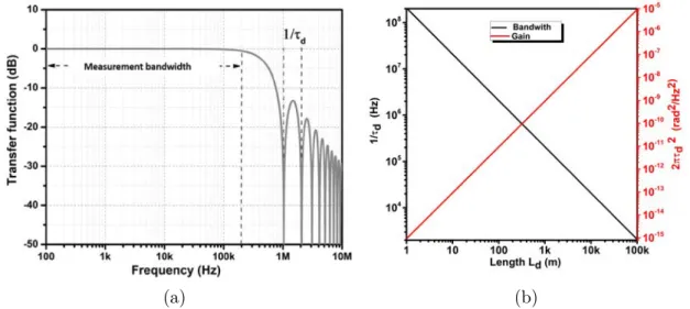
1.6 (a) Transfer function of an unbalanced interferometer (τd= 200 m) (b) Cutoff

frequency and gain conversion of the test bench, depending on the inserted

delay length. . . 22

1.7 Experimental setup for noise floor measurement. OC: Optical coupler, PC:

Polarization controller, AOM: Acousto-optical modulator, PD: photodetector,

TIA: Transimpedance amplifier, SSA: Signal source analyzer. . . 22

1.8 (a) Phase noises of the laser and noise floors of the bench for different fiber

lengths. (b) Frequency noise measurement of the Tunics OM laser and its

linewidth estimation using β − line approximation. . . . 24

1.9 General scheme for frequency stabilization of a laser. . . 25

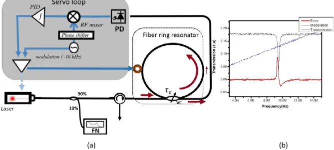
1.10 (a) General scheme of top-of-fringe frequency stabilization. (b) Oscilloscope traces for transmission laser signal, modulation and top of fringe error

sig-nals. PD: photodetector, PID: Proportional–integral–derivative controller,

VC: Variable coupler, FN: Frequency noise measurement bench. . . 28

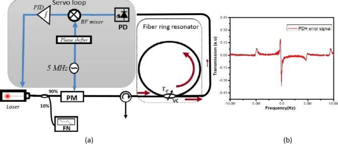
1.11 (a) General scheme of PDH frequency stabilization. (b) Experimental Oscillo-scope traces for PDH error signal. PM: Phase modulator, PD: photodetector, PID: Proportional–integral–derivative controller, VC: Variable coupler, FN:

Frequency noise measurement bench. . . 29

1.12 (a) Frequency noise measurement of the stabilized Tunics laser on fiber ring

cavity with top of fringe and PDH lock. . . 30

2.1 Schematic representation of Brillouin scattering process and schematics

dia-gram of (a) the propagation direction and (b) Momentum conservation of the incident, scattered (Stokes in orange) and acoustic wave. Red dashed lines

(14)

List of Figures xiii

2.2 Stokes process in (a) the spontaneous regime. Amplitudes of Stokes and

anti-Stokes are of same order. (b) Stimulated Brillouin scattering regime. anti-Stokes

amplitude will increase and its gain spectrum narrows. νB: Brillouin shift,

νP: pump frequency, ∆νB: Brillouin gain bandwidth and gB: Brillouin gain

coefficient . . . 36

2.3 Schematic representation of the SBS. The beat between the pump wave and

the Stokes wave creates by electrostriction and acoustic wave that diffuses the

pump wave and therefore reinforces the Stokes wave. . . 37

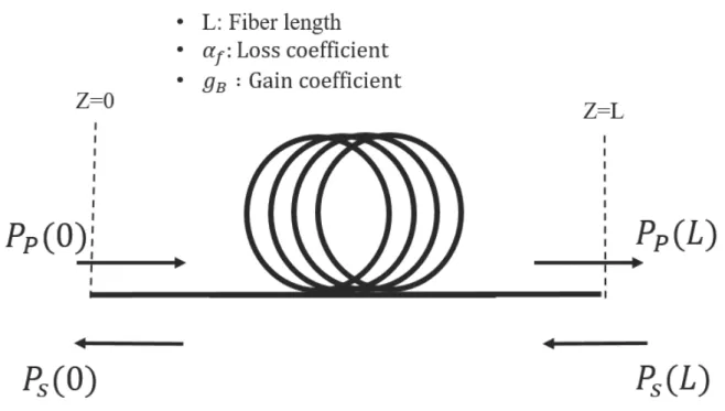
2.4 Schematics of the pump-probe method. Pp and Ps are the pump and Stokes

powers respectively. . . 39

2.5 Definition of Brillouin threshold power using transmitted (red) and back

scat-tered Stokes (black) signals plotted as a function of the input power. 1 % of

the input signal is plotted in blue color for references. Pp(0) : input pump

power, PS(0): back-scattered Stokes, Pp(L): transmitted power; (a)

Logarith-mic scale (b) Linear scale. . . 40

2.6 Experimental setup of self-heterodyne technique for measuring the Brillouin

gain bandwidth. EDFA: Erbium doped fiber amplifer, VOA: Variable optical attenuator, PM: Powermeter, FUT: Fiber under test (L=26 km), PC: Po-larization controller, PD: Photodetector, ESA: Electrical Spectrum Analyzer,

OC: Optical coupler. . . 44

2.7 (a) Spontaneous Brillouin spectrum at -6.8 dBm with Lorentzian fit. (b)

Stimulated Brillouin spectrum at 9.2 dBm with Gaussian fit. . . 45

2.8 FWHM of Brillouin spectra as a function of the input pump power in SMF-28

fiber. . . 46

2.9 Experimental setup for SBS threshold measurement. EDFA: Erbium doped

fiber amplifer, VOA: Variable optical attenuator, FUT: Fiber under test (L=26

km), PM: Powermeter, OC: Optical coupler. . . 47

2.10 Brillouin threshold estimation using L-I curve measurement for a 26 km long

SMF-28. . . 48

2.11 Schematic view of the resonator. Sin(t) : input field, Sout(t) : output field,

u(t) : resonant field, τ0 : intrinsic photon lifetime, τe : coupling lifetime. . . 50

2.12 (a) Transmission spectrum in steady state for different relative values of τ0

and τe [1]. (b) Transmission at resonance T(δ=0) in decibels as a function of

1/τ0 for the different coupling regimes. . . 52

2.13 Transmission of a resonator for different scanning speeds.(a) ˜VS=0.0075 ˜V0,(b)

˜

VS=0.3 ˜V0, (c) ˜VS=3 ˜V0, (d) ˜VS=30 ˜V0 with a ˜V0 = 2/(πτ2) [1]. . . 56

2.14 (a) Transmission in the stationary regime as a function of the normalized

detuning in the case of τ0 = 3τe and τe = 3τ0. The two curves are exactly

superimposed. (b) Transmission as a function of time in the same two cases

with Vs= 2.25V0. Note that the two responses are easily distinguishable [1]. 57

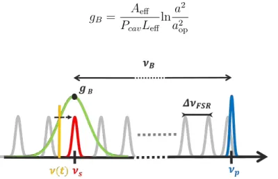
2.15 Spectral overview of the CRDM method: Pump laser line (blue), Brillouin gain curve (green), probed cavity mode (red) and probing laser line (yellow).

νB corresponds to the Brillouin shift, where ∆νF SR stands for the spectral

spacing (Free Spectral Range) between cavity modes. . . 57

2.16 a) Experimental setup for Brillouin gain cavity ringdown determination. EDFA: Erbium-doped fiber amplifier, VOA: Variable optical attenuator, OC : Opti-cal coupler, PC: Polarization controller, BOSA: Brillouin optiOpti-cal spectrum

(15)

xiv List of Figures

2.17 Fast scanning profiles recorded from the Brillouin cavity at different pumping

power (Pin) with a scanning speed of 2.8 M Hz/µs: The intrinsic photon

lifetime (τ0), transmission and Brillouin gain coefficients are deduced from

the analytical fits (red) of experimental curve (black). (a) cold cavity, (b) under coupling, (c) near to critical coupling, (d) over coupling, (f) near to

transparency, (g) amplification. . . 60

2.18 Resonant transmission obtained from the fitting of ringing profiles in the

Bril-louin cavity. This figure is inspired from article [2]. . . 62

2.19 Brillouin gain coefficient extracted from the CRDM signal for various input

pump powers. The mean value is equal to gB = 1.94×10−11±1.5×10−12m/W . 62

3.1 Distribution of cavity modes under the Brillouin gain curve. . . 72

3.2 Schematic representation of a BFL cavity with non-resonant pumping showing

the different losses coefficients detailed in table (3.1). . . 75

3.3 Experimental setup for non-resonant fiber ring cavity Brillouin laser

charac-terization . . . 76

3.4 (a) Optical spectrum and (b) Power characterization of the 20 m non-resonant

BFL cavity . . . 77

3.5 Mode-hopping of non-resonant Brillouin laser cavity, observed through a

Fabry-Perot analyzer in different time intervals (black signal). Red signal shows that

we can observe two resonant modes at the same time under the gain bandwidth. 78

3.6 Experimental setup of BFL cavity with active PDH locking on cavity a

res-onances. EDFA: Erbium-doped fiber amplifier, VOA: Variable optical atten-uator, OC: Optical coupler, PD: Photodetector, PM: Phase modulator, OI:

Optical isolator, OF: Optical filter. . . 79

3.7 (a) Beating between pump and Stokes wave with and without mode-hopping

stabilization scheme. (b) Optical spectrum of stabilized non-resonant BFL

cavity. . . 80

3.8 Analytical phase noise transfer function for the 20 m fiber length cavity with

R = 0.78 and βA = 17.27. . . 82

3.9 Experimental and analytical frequency noise measurement of 20 m non-resonant

BFL. Corresponding noise floor with 200 m delay is plotted in dotted line. . 84

3.10 Frequency noise of the non-resonant BFL laser. (a) pump and Stokes sig-nal with and without stabilization in logarithmic scale (b) frequency noise of

cascaded non-resonant BFL laser in linear scale. . . 86

4.1 Illustration of cascade Brillouin laser. A pump laser of frequency ω0 is

in-jected into an optical resonator. When its wavelength matches the Brillouin

condition ((ΩB/2π) = N × ∆νF SR), pump resonant mode at ω0 is scattered

at ω1 by emitting a phonon at ΩB. When the pump power is sufficiently high,

the Stokes wave at ω1 acts as a pump for higher order Stokes lines. . . 91

4.2 Experimental setup to study the lasing properties of multi-Stokes Brillouin

Laser. Pump: Koheras continous wave laser, EDFA: Erbium-doped fiber am-plifer, VOA- variable optical attenuator , VC: Variable coupler, PZT: Piezo-electric transducer, Filter: Yenista optical filter, PD: Photodetector, PID: Proportional-integral differential amplifier, HV: High-voltage amplifer, TA: Transimpedance Amplifier, ESA : Electrical spetrum analyzer. 20 m polar-ization maintaining fiber spooled in PZT. Red line: Pump wave, Blue: Stokes

(16)

List of Figures xv

4.3 Steady-state laser powers for the Stokes components, obtained from the

sim-ulation. . . 96

4.4 (a) Power characterization of M BLLQ cavity (b) Normalized Power

charac-terization of M BLLQ cavity with its input power, Pc: clamping power, Pth:

threshold power of S1. . . 98

4.5 Power characterization of M BLHQ cavity. . . 98

4.6 Left axis : Output Stokes power (Ps) normalized to the circulating power (Pc)

versus input pump power (Pin) normalized to the Stokes 1 lasing threshold

(Pth). Right axis: RIN of Stokes lines normalized to the input pump RIN.

RIN amplitude is measured at 4 kHz from the carrier. Straight lines and full dots are experimental results. Stars are simulation results. Results are

obtained with the "low-Q cavity" Brillouin laser, Pth= 26.5 mW. . . . 102

4.7 Relative intensity noise reduction of the MBL Stokes1 when it is compared

to the pump (a) Brillouin laser S1 intensity noise decreases with the injected

pump power. (b) RIN of S1 normalized by the pump RIN. . . 104

4.8 Relaxation frequency as a function of the normalized pump power for

low-Q (light blue) and high-low-Q (deep blue) cavities. Lines represent the results of calculation of Eq. (4.10). Error bars (±75 kHz) represent the possible

misreading of relaxation frequency on RIN curve. . . 105

4.9 Normalized RIN of Stokes 1 (a, b) and Stokes 2 (c, d) lines for various input

pump power. Full and dashed lines hold for experimental and simulation

results respectively. Deep and light colors refered to high (τ0 = 1.4 µs, τe =

3.7 µs) and low-Q factors (τ0 = 1.4 µs, τe= 0.5 µs) respectively. . . . 106

4.10 Schematic presentation of frequency fluctuations converted into intensity

fluc-tuations cavity Q-factors. . . 107

4.11 Schematics presentation of gain detuning of Brillouin cavity. . . 109

4.12 Evolution of the Stokes 1 RIN as a function of the gain detuning for a pump

power of a) 5.5 Pth and b) 9 Pth in the low-Q cavity configuration. . . 110

4.13 Experimental setup for gain detuning measurements; Koheras laser (brown) creates Brillouin scattering (dark blue) in the cavity and the probe laser (light blue) slowly scans the Brillouin gain. b) In the inset, different optical spectra

measured thanks to an oscilloscope are given for different input pump powers. 111

4.14 Experimental setup of the BFL cavity with PDH locking. . . 114

4.15 BFL detuning measurement: The measured Brillouin frequency shift (squares)

and S1 threshold (dot) are plotted as a function of pump wavelength. . . 115

4.16 Schematic of anti-Stokes generations in cascaded Brillouin laser; dotted line : resonance of the cavity; shaded spectrum are Brillouin gain profiles for Stokes and anti-Stokes: S1 (blue), S2 (green), S3 (yellow); sharp peaks are Stokes

stimulated laser lines and pump (green for S2, blue for S1, red for the pump). 117

4.17 Theoretical results from [3] showing the degradation of linewidth of different

Stokes components due to AS. This degradation can be equivalently observed

in frequency noise (chapter 1, section 1.4.2). . . 118

4.18 Cascaded Brillouin laser frequency noise dynamics (a) S1 frequency noise at different pump powers in linear scale (b) S1 white noise at a fixed frequency

of 200 kHz as a function of normalized pump power. . . 118

4.19 (a) S1 frequency noise (b) S2 frequency noise for different regimes. . . 121

4.20 The pump frequeny noise to Stokes frequency noise (a) zero detuning (b) with

pump and SBS gain detuning [4]. . . 122

(17)

xvi List of Figures

4.22 Impact of the photon lifetime in S1 frequency noise at a given pumping rate 125

A.1 (a) Schematic representation of spontaneous emission of laser field (b) Contri-bution of stimulated emission generated by optical amplification and filtered

by an optical cavity. . . 133

C.1 Representation of the Brillouin gain and side mode suppression . . . 138

(18)

xvii

List of Tables

2.1 Parameters obtained from the fitting of ringing profiles at different pump powers 61

2.2 Comparison of gB values obtained for single mode silica fibers [5] in various

works. SH stands for self-heterodyne. . . 63

2.3 Material values for pure and 3% GeO2 doped silica fibers. . . 63

2.4 Parameters of a 3% GeO2 doped silica fibers . . . 64

3.1 Losses coefficients of each components in the cavity . . . 75

3.2 Parameters of the non-resonant BFL cavity . . . 76

4.1 Parameters of resonant BFL 20m cavity . . . 93

4.2 Threshold of resonant BFL cavity . . . 99

4.3 Comparison of S1 linewidth in different cavities . . . 125

(19)

1

Introduction

In 1922, Léon Brillouin theoretically predicted the scattering due to the interaction of

the photons and acoustic waves (propagating density fluctuations) [6]. The experimental

verification was difficult at that time due to the lack of coherent light source to efficiently

generate an ultrasonic pressure wave. In 1930, Gross [7] experimentally proved the

ex-istence of photon and acoustics wave interaction. Gross was originally looking for the Raman scattering in organic liquids, but his measurements did not agree with Raman scattering. However it perfectly matched the theoretical predictions made by Brillouin.

Note that Mandelstam predicted a similar scattering effect in 1926 [8]. Based on the work

of Leon Brillouin, the inelastic scattering of the light from acoustic waves is referred as Brillouin scattering in literature.

The discovery of the laser (light amplification by stimulated emission of radiation) in the 1960s, revolutionized the study of fundamental physics by giving birth to new research like laser physics, nonlinear optics, etc. The lasers provide a coherent and powerful light source, that leads to changes in the material properties. Nowadays, lasers play vital role in telecommunication, medicine, defense, industry, environment, lightning ... In recent decades, different types of lasers have been developed in terms of optical power, coherency and wavelengths.

Soon after the first realization of a laser [9], Chaio and Townes observed, in 1964,

stimulated Brillouin scattering (SBS) in quartz and sapphire [10]. After the invention

of optical fibers, stimulated Brillouin scattering was first studied in 1972 by Ippen and

Stolen [11]. Then SBS gained attention in telecommunication systems because it limits

the performances by reflecting most of the power through the counter-propagating Stokes wave. It results in large depletion of pump power. On the contrary SBS can be used

on purposes as optical amplifiers [12], lasers [13], filters [14, 15], and sensors [16, 17].

(20)

2 List of Tables

the field of Brillouin based bio-imaging [18, 19, 20]. In the past century, a tremendous

amount of research was done concerning Brillouin scattering, especially in the last decades

during which, SBS was observed in chip-scale structures [21, 22], and different materials

like silica [11], chalcogenide [23], tellurium [24].

In 1976, Hill [13] realized a fiber laser based on Brillouin effects, which had the unique

ability to reduce noise compared to that of the pump [25]. Later, different architectures of

Brillouin lasers [26,25,27,28,29,30,31,32] are studied. This low-noise laser is of interest

to the scientific community for applications in microwave and optical signal processing, distributed sensors, spectroscopy, gyroscope, metrology. The noise properties of this laser are not well understood. In this thesis, we explain two Brillouin laser architectures: resonant and non-resonant Brillouin laser and their noise properties.

Objectives of the thesis

This thesis is devoted to the understanding of ring Brillouin fiber lasers, operating with multiple Stokes orders. Most of the work carried out during this thesis is part of the

continuity of the works of Kenny Tow [33] and Schadrac Fresnel [34]. My work was

accomplished in the framework of the SOLBO project (SOurces Laser Brillouin cOhérent à faible bruit) of the FUI call (Fonds Unique Interministériel AAP20) with the help of BPI France, the "Images et réseaux" cluster and in collaboration with IDIL Fibre Optiques (project leader), Lumibird, THALES, ISCR (Institut des Sciences Chimiques de Rennes), Photonics Bretagne.

The main objective was to design a low cost Brillouin fiber laser, with an integrated linewidth below kHz, by IDIL and also for the Foton Institute, to explore the physics of multi-Stokes Brillouin fiber lasers and to try to know the fundamental limitations of frequency noise reduction for these sources, whether for single or multiple Stokes order cavities. In this thesis, I propose

• a new Brillouin gain measurement technique, particularly adapted to short cavities and not requiring high optical pump powers (a few tens of milliWatts),

• a comparison of laser operation between resonant and non-resonant pumping, • a modeling of our experimental results by an analytical approach, allowing us to

(21)

List of Tables 3

• a discussion of the fundamental limitations of these devices and their advantages.

Main results

Firstly, we will report a technique based upon the cavity ring-down method that enables the characterization of the Brillouin gain coefficient directly from probing the laser cavity. Material gain, optical cavity parameters, and lasing properties can be extracted from measurements within a single experiment. This method could be used to characterize an integrated microresonator Brillouin cavity. Secondly, we will study two different Brillouin designs, which are using resonant or non-resonant pumping. In non-resonant Brillouin laser, the pump is doing a single pass inside the cavity, and the generated Stokes wave are resonant inside the cavity. In order to increase the long-term stability of such scheme, we will propose a frequency stabilized non-resonant Brillouin fiber laser design, that enables us to compare our analytical and experimental results about frequency noise in a non-resonant Brillouin laser. The intrinsic linewidth of our non-non-resonant Brillouin laser is 1.3 Hz. Furthermore, we demonstrate experimentally that the intrinsic linewidth can be reduced down to 47 mHz by cascading two non-resonant Brillouin lasers, showing the ease and ability of such systems to produce low-noise light. Unfortunately, we did not succeeded to explore the fundamental limitations of noise reduction due to the noise floor of our bench.

A major work of this thesis is the investigation of noise properties of a resonant Brillouin laser. For resonant pumping, the pump and Stokes waves are resonant inside the cavity, which could produce multi-Stokes orders. We experimentally analyze, in this cascaded regime, steady-state optical powers and noise properties of the different signals, including frequency noise and relative intensity noise. Our experimental results reveal that the cascading process modifies the dynamics of Brillouin laser when compared to those of single-mode Brillouin laser with a single first order Stokes component.

We analytically and experimentally investigate the intensity noise of each Stokes wave and study the noise dynamics of the cascaded Brillouin scattering process. In particular we examine the impact of fiber ring quality factor on the laser RIN features such as amplitude-noise reduction and relaxation frequency. We also investigate the influence of the Brillouin gain detuning on the RIN reduction. This detailed study is important as many characteristics of frequency noise are related to RIN properties through a coupling

(22)

4 List of Tables

between intensity and phase.

The study of frequency noise dynamics of a multi-Stokes Brillouin fiber laser was done on a large mode-volume optical resonator with 2 m optical cavity, because this kind of cavity is less sensitive to acoustical and thermal fluctuations than micro-cavity. It will enable to reach lower flicker noise. With this cavity, we have reached an intrinsic linewidth of 12.8 Hz and less than 2 kHz integrated linewidth for 10 ms observation time. Furthermore, we will experimentally demonstrate for the first time that the frequency noise is increased in the presence of anti-Stokes Brillouin scattering in the cascading process. We will also show that the gain detuning could enhance the linewidth by an amplitude-phase coupling. All these experimental results are in good agreement with our analytical calculations obtained through our nonlinear system for multi-Stokes Brillouin laser. This good match is mainly due to three facts:

1. we are able to get directly very precise values of cavity parameters and of the Brillouin gain coefficient using the CRDM technique;

2. we are able to reach long term stability (tens of hours);

3. we are able to finely control the detuning between the laser Stoke resonance and the frequency of Brillouin gain maximum.

All these very fine observations allow us to design and engineer Brillouin fiber lasers. We show some fundamental limitations of these systems in terms of noise reduction such as

• the role of pump noise, possibly in its interrelation with cavity finesse,

• anti-Stokes orders,

• the effect of detuning is inherent in higher Stokes orders.

Nevertheless, such systems are still very pervasive as evidenced by the interest they arouse in the scientific community. This Ph.D. thesis contributes to a better understanding of multi-Stokes Brillouin lasers.

(23)

List of Tables 5

Thesis organization

This thesis is organized into four chapters followed by a conclusion and some remarks. In chapter 1, we give a general introduction to the physics of laser noise necessary to understand the work of this manuscript. It also details the measurement technique for frequency noise and relative intensity noise (RIN) of laser. Moreover, we introduce fun-damental ingredients of the laser stabilization methods, which have been used for the realization of Brillouin laser.

Chapter 2 begins by describing physical mechanisms behind the Brillouin scattering in optical fibers. We will briefly describe spontaneous and stimulated Brillouin scatter-ing and will explain a new Brillouin gain characterization based on the cavity rscatter-ing-down method (CRDM). We will also compare the results with conventional Brillouin gain char-acterization. This cavity ring-down method enables us to identify the different coupling regimes and estimate the Q-factor of the resonator. These measurements are fundamental to characterize Brillouin laser cavity and ease to design Brillouin cavity.

In chapter 3, we will describe a stabilized non-resonant Brillouin laser. The chapter begins with a historical overview of Brillouin lasers. This overview explores different laser designs and current state of the art of Brillouin lasers in fiber, integrated chip, and microresonator. Moreover, we address the issue of mode-hopping in non-resonant Brillouin laser and propose a frequency stabilization method based on Pound–Drever–Hall (PDH) locking. Also, we investigate the power and frequency noise characterization of non-resonant Brillouin laser. We show experimental frequency noise agreement to analytical results and corresponding laser linewidth are in the range of Hz level. We demonstrate that the cascading of two Brillouin lasers can reach the mHz linewidth.

In chapter 4, we will explore the physics of resonant Brillouin laser. We will discuss the power and noise dynamics of theses lasers with the help of our numerical and experimental results. RIN of resonant Brillouin lasers will be studied in terms of pumping power, photon lifetime, and gain detuning in the so-called single-mode and cascading regimes of the laser. We will show that our numerical simulations and experimental results are in good agreement. We will discuss some fundamental limitations of noise reduction linked to pump noise, Q-factor, anti-Stokes orders, gain detuning and amplitude phase-coupling.

(24)

(25)

7

Chapter 1 Noise in lasers

1.1 Introduction

Narrow linewidth lasers are of great importance for several areas, such as coherent

opti-cal telecommunications [35, 36], sensors [37], precision spectroscopy [38], optical atomic

clocks [39,40], frequency metrology [41,42], LiDAR [43] and microwave photonics [44] to

only name a few. My work is mainly focused on the development of low-noise Brillouin laser; the study of these lasers demonstrates that it is possible to produce a laser output with low-noises when compared to those of the pump laser. But before explaining this, it is necessary to introduce the theoretical and experimental basics of laser noises, which

are available in many books [33, 34, 45, 46, 47, 48,49, 50]. The object of this chapter is

to introduce laser noises descriptions. The origin of the laser noise is defined and

intro-duced, in section (1.2), by considering the amplitude and phase noises. In section (1.3),

theory and experimental measurement methods are explained for laser relative intensity

noise (RIN) while section (1.4) is dedicated to laser phase noise. Moreover, theoretical

and experimental basics of the linewidth narrowing method, which is based upon laser

frequency-stabilization on fiber ring cavity are introduced in section (1.5).

1.2 Origin of noise in lasers

In a laser, spontaneous emission plays an essential role in the generation of initial pho-tons that leads to amplification by stimulated emission, and that will gives the laser emission. The spontaneous emission is a random process, which emits photons with

(26)

8 Chapter 1. Noise in lasers

random direction, phase and polarization. These random fluctuations are called intrin-sic or fundamental "noise" of the laser. These fluctuations may have a negative impact on numerous laser applications, more particularly in the field of metrology and optical sensors.

In presences of noise, the scalar electric field associated with the light wave, delivered

by a single mode laser at the optical frequency of ν0, is written:

E(t) = [E0+ δE(t)]ei[2πν0t+φ(t)] (1.1)

Where δE(t) and φ(t) are temporal fluctuations of amplitude and phase. The represen-tation is linked to the Fresnel vector in the complex plane (It is explained in appendix

(A) [50]). The origin of these fluctuations can be classified into two categories: the first

one is at the quantum level; this fundamental noise comes from the spontaneous emission process in lasers. The electromagnetic thermal radiation will also contribute to fluctua-tions. The second one is called technical noise; it may include several contributions as : acoustical and mechanical vibrations, temperature fluctuations or even the pump noise. Theses various random contributions lead to amplitude and phase noises that will be studied through their power spectral density (PSD).

PSD of a given random variable, δb(t) (to be more general), will be the Fourier

transform of its autocorrelation function Rδb. b can be either intensity or phase in the

present study. The PSD can be written as Sδb:

Sδb(f ) =

Z +∞

−∞

Rδb(τ )e−i2πf τdτ (1.2)

with Rδb being the autocorrelation function of δb(t) defined by

Rδb(τ ) =< δb(t)δb(t − τ ) >=

Z +∞

−∞ δb(t)δb(t − τ )dt (1.3)

Note that in Eq.(1.2) the frequencies of interest are mainly in the electrical domain [DC

to a few GHz]. For that reason f may be used instead of ν to indicate low frequency components. It’s why the measurements are carried out in the electrical field rather than in the optical field by an electrical spectrum analyzer (ESA). In the next sections, we will define amplitude and phase noises and explain the associated measurement methods to characterize them.

(27)

1.3. Relative intensity noise (RIN) 9

1.3 Relative intensity noise (RIN)

One of the objectives of this thesis is to study the intensity noise of a Brillouin laser experimentally and theoretically. In particular, we experimentally analyze the intensity noise of each Stokes wave generated through the Brillouin process. We examine the impact of the cavity parameters on the laser RIN features. In this section, we introduce the RIN principles and measurement method, some of the notations and explanations are

taken from the following references [33,34].

1.3.1 Definition of relative intensity noise

The emitted laser field (Eq.1.1) has temporal amplitude fluctuations; the related optical

power as well:

P (t) = P0+ δP (t) (1.4)

where P0 is the average power and δP (t) is the temporal fluctuation of optical power. It

describes the fluctuations of the optical power output of the laser around its average power

of P0. The intensity noise is obtained by dividing the optical power by the effective area,

which is the illuminated surface. Then the laser relative intensity noise can be defined by taking a Fourier transform of δP (t)

RIN (f ) = h| δP (f ) |

2_i

P2 0

(1.5) hi stands for statistical expectation. Thus the RIN is defined by the ratio of the power

spectral density SδP 1 over the average optical power. SδP is the Fourier transform of the

auto-correlation of δP (t) and is related to the second moment of the noise forces. The definition can be taken in the electrical domain:

RIN (f ) = SRIN Pele

(1.6)

Where SRIN is the electrical power spectral density. Pele is average electrical power.

The relation between optical power and electric power Pele = RI02 = Rη2P02; R is the

load resistance of the photodetector. I0 is the average photocurrent produced by the

photodetector. η is the quantum efficiency of the photodetector. In the following, the RIN measurement method used in this manuscript is described.

1_S

(28)

1.3.2 RIN measurement method

At Institut FOTON, we study the intensity noise by a direct detection of PSD using an

electrical spectrum analyzer [33, 34]. The experimental setup used to characterize the

RIN of a laser during this thesis is shown in figure (1.1).

Figure 1.1: RIN measurement setup. The photocurrent from the photodetector is mea-sured and amplified. Its DC component is blocked before its spectral analysis by the ESA. PD: photodetector, TIA: Transimpedance amplifier, ESA: Electrical spectrum analyzer.

The RIN detection system consists of a photodetector with a bandwidth from DC to 1 GHz, a trans-impedance amplifier (TIA) with a variable bandwidth depending on the gain, but not exceeding 200 MHz, and a "DC-Block" module with very low cut-off frequency (1 Hz), to remove the DC component of the electrical signal in order to avoid damaging the ESA. PSD is analyzed with the help of the ESA. The PSD collected on the

ESA contains not only the PSD of the RIN but also that of thermal noise (ST) and shot

noise (Ssh). The PSD detected at the electric spectrum analyzer is then the sum of these

three noise sources. As they are independent stochastic processes, the total PSD can be written as:

ST otal = ST + Ssh+ SRIN (1.7)

It is then necessary to measure the thermal and shot noise contributions in order to obtain the laser RIN. It will be explained in the next section.

1.3.3 Determination of thermal noise

Thermal noise ST is independent of the optical signal received on the detector but

de-pends on the devices in the measurement system (ESA, photodetector, amplifier). It is simply measured without an optical signal on photodetector. It consists of two main con-tributions: thermal noise (or Johnson noise or Johnson-Nyquist noise) and flicker, called also excess or 1/f noise. In the case of a photodetection system, even in the absence of

(29)

1.3. Relative intensity noise (RIN) 11

the incident signal, a current is generated by the movement of the charge carriers in the material due to thermal agitation. These current fluctuations induce thermal noise. The PSD of fluctuations due to thermal noise can be expressed as

ST = 4kBT B (1.8)

where kB = 1.3807.10−23 J/K is the Boltzmann constant, T is the temperature given

in Kelvin and B is the detection bandwidth. The PSD of the flicker noise is linked to electronic components (photodetector, amplifiers, ESA) that are used to measure. This

noise is the consequence of several random processes [51]: fluctuations in the number

of carriers [52], fluctuations in the mobility of carriers [53]. It is due to the presence of

impurities and structural defects during the manufacture of electronic components. So this noise depends on the quality of the manufacturing and the technology employed. In the case of semiconductors, this noise can become annoying for frequencies below a few kHz. Thermal noise is the minimum signal level measurable by the detection bench and then have to be reduced by a judicious choice of devices.

1.3.4 Determination of shot noise

Shot noise (Ssh) is related to the randomness of the photons and electrons during the

creation of photocurrent in the photodetector. The photocurrent is a function of the incident optical power. The PSD of shot noise is related to the photocurrent. If H(f ) is the transfer function of the detection chain, then the PSD of the shot noise is written as

[54]:

Ssh = |H(f )|22qRI0 (1.9)

where R is the load resistance of the spectrum analyzer. q is the electronic charge equal

to 1.602 × 10−19 coulomb, and I0 is the average photocurrent.

To evaluate the shot noise, it is necessary to use a reference source having a negligible

intensity noise with respect to that of the shot noise [55]. White light sources are good

candidates for this measurement [33,34]. To ensure that the detection is at the level of the

shot noise, we check the linearity of the measurements with the photocurrent. If the rel-ative intensity noise is not negligible, we will have a non-linear behavior. Quantitrel-atively, the shot noise PSD normalized by the photocurrent is given by the relation:

Sshnorm = |H(f )|

(30)

Then the transfer function of the detection system can be written as:

|H(f )|2 ₌ Sshnorm

2qR (1.11)

From these thermal and shot noise PSD determination, we can calculate the RIN, as it will be explain in the next section.

1.3.5 Determination of relative intensity noise

The spectral density of the laser intensity noise is given by the following relation:

SRIN = |H(f )|2RI210RIN/10 (1.12)

RIN is expressed in dBc/Hz and by abuse of use dB/Hz is used. The RIN of a laser can

be obtained by insertion of Eqs. (1.12), (1.11), (1.10) in Eq (1.7):

RIN = 10 log₁₀ 2q I " ST otal− ST SshnormI − 1 #! (1.13)

Figure (1.2) shows an example of RIN spectrum of a DFB fiber laser (KoherasT M₎

emitting at a wavelength of 1.55 µm that will be used as a pump laser in the following chapters of this thesis. The peak around 154 kHz corresponds to the relaxation frequency of the laser. Beyond this frequency, the PSD decreases very quickly with a slope of 20 dB per decade. RIN is usually low in laser due to the clamping of the gain that reduces

Figure 1.2: RIN of a DFB fiber laser (Koheras) emitting at a wavelength of 1550 nm

the input pump noise. This feedback mechanism is not present on the phase of the laser that continuously drifts and implies a larger noise contribution than in amplitude. The phase noise is explained in next sections.

(31)

1.4. Phase noise 13

1.4 Phase noise

In this section, we review the basic concepts of phase and frequency noises of a laser. We also describe the relations between the phase noise, frequency noise, and spectral laser linewidth. Moreover, we explain the measurement method of laser frequency noise based on the self heterodyne technique.

As we have seen in section (1.2), if we consider the laser emission as a perfect signal

E(t) = E0ei[2πν0t], then the power is concentrated at a carrier frequency ν0, the optical

spectrum will be a Dirac function. But as a matter of fact, a sinusoidal signal has infinite energy and a more precise description will consider a broader emission with finite energy. Then, laser signal will fluctuate randomly in phase so the total power of the

signal is symmetrically distributed on each side of the frequency ν0. The full width at

half maximum (FWHM) of the energy distribution is called the laser linewidth. According

to the theory of Schawlow and Townes [56], the linewidth of a laser is due to phase noise

caused by spontaneous emission of photons in a laser cavity. This fundamental limit of a laser linewidth can be described by a Lorentzian spectral lineshape:

∆νL=

πhν

(2δ1/2)2P0

(1.14)

Where hν is the photon energy, 2δ1/2 is the laser cavity resonance width and the P0

is the laser output power. Generally, this value is very difficult to measure from the optical spectrum because other technical noise may increase the laser linewidth such as acoustical and mechanical vibrations, mode beatings between different longitudinal or transverse modes and noise transfer from the pump sources to the laser. In semiconductor laser this linewidth will be higher because of the coupling between intensity and phase, which is caused by the refractive index dependence on the carrier density. The study of the phase or frequency noises will give information about the Lorentzian linewidth of the laser and other contributions like Gaussian distribution due to environmental noises. Laser phase noise is characterized in the electrical domain with a single side-band power

spectral density Sφ(f ). In the following subsections, we will firstly introduce the relation

between phase and frequency noise. Then we will explain the linewidth determination from the frequency noise underlying different noises like white and flicker noise in section

(32)

noise using the self-heterodyne method. The inherent noise floor of the experimental bench is analyzed.

1.4.1 Frequency noise in laser

The spectral purity of the laser can be expressed as a function of frequency. The instan-taneous frequency of the laser is:

ν(t) = ν0+ δν(t) (1.15)

Where ν0 is the central frequency. δν(t) is related to the fluctuation of the frequency and

phase by δν(t) = _2π1 dφ(t)_dt . ν(t) = 1 2π d dt[2πν0t + φ(t)] = ν0+ 1 2π dφ(t) dt (1.16)

PSD of the frequency fluctuations δν(t) can be obtained by Eq (1.17):

Sν(f ) =

Z +∞

−∞

Rν(t)(τ )e−i2πf τdτ (1.17)

with Rν(τ ) being the autocorrelation function of δν(t) defined by

Rν(τ ) =< δν(t)δν(t − τ ) >=

Z +∞

−∞ δν(t)δν(t − τ )dt (1.18)

Sν(f ) is expressed in Hz2/Hz. The relation between the phase and frequency noise

is then linked through a derivative in the time domain, which implies, for the PSD, a proportional factor equal to the square of the frequency:

Sν(f ) = f2Sφ(f ) (1.19)

In general, PSD of laser frequency noise can be expressed in the form :

Sν(f ) =

h−1

f + h0 (1.20)

Where h0 is a white noise contribution (due to spontaneous emission). h−1_f is the laser

flicker noise. These two contributions are the main ones in lasers. However the −1 term

may be replaced by h−2_f2 , which is linked to a random walk frequency noise (a term

h−α fα

with 1 < α < 2, may be also added or it may replace h−1_f ). It is interesting to know

how to relate the frequency noise obtained from the noise PSD and the laser linewidth

(33)

1.4. Phase noise 15

1.4.2 Relation between the power spectral density of

frequency noise and optical spectrum

In this section we present a simple approach to estimate the laser linewidth from the

frequency noise, a detailed explanation can be found in [57, 58, 59]. If we consider that

the laser field is written as E(t) = E0ei(2πν0t+φ(t)), neglecting the intensity noise δE(t) = 0,

then the PSD of its frequency noise is linked to the auto-correlation function as follows:

RE(τ ) = E02e i2πν0τ e−2 R+∞ 0 Sν(f ) sin2(πf τ ) f 2 df _(1.21)

The laser spectrum is obtained by performing a Fourier transform:

SE(ν) = 2

Z +∞

−∞

e−i2πντRE(τ )dτ (1.22)

As we have seen before a laser frequency noise PSD may be the sum of three types of noise: white, flicker, and random walk. In this thesis, we are focused only on white and flicker noises. In the following, we will detail the contributions of the white and flicker noises separately. Finally, we will explain the general case, which includes both noise contributions in the laser spectrum. The linewidth associated with the white noise is called intrinsic linewidth.

White noise

Let consider that the laser emission is only under the influence of spontaneous emission

(white noise), then the PSD of the frequency noise (Eq1.20) reduces to Sν(f ) = h0. The

optical spectrum Eq (1.22) is then written as:

SE(ν) = E02

h0

(ν − ν0)2 + (πh0/2)2

(1.23) The laser spectrum has a Lorentzian shape. Its FWHM is the laser intrinsic linewidth.

∆νL = πh0. In figure (1.3) plotted the white frequency noise and its optical

spec-trum. The white frequency noise is plotted for a value h0 = 104 Hz2/Hz corresponding

Lorentzian shape spectrum is give a intrinsic linewidth ∆νL = 31.4 kHz. In this thesis

manuscript, this relation is used to determine the intrinsic linewidth of a Brillouin laser.

(34)

(a) (b)

Figure 1.3: Illustration of corresponding frequency noise and optical spectrum.(a)

Fre-quency noise Sν(f ) = h0 = 104 Hz2/Hz. (b) Optical spectral of the laser corresponds to

the white frequency noise and the intrinsic linewidth ∆νL = 31.4 kHz

Frequency fliker noise is slighty more difficult to handle than in the case of white

noise. Considering the flicker noise PSD is Sν(f ) = h−1_f . Then Eq.(1.21) is written as

RE(τ ) = E02e

i2πν0τ_e−2R0+∞h−1(f )

sin2(πf τ )

f 3 df _(1.24)

In this expression we can see that the integral ( J =R+∞

0 h−1(f )sin

2_{(πf τ )}

f3 df ) is not defined

at f = 0 but it can be shown [57] that it is a finite integral with an asymptotic value

σ2 _{= 3.56h}

−1, in which σ2 is linked to the width of the integrated linewidth.

In order to simplify this problem, we may introduce the notion of observation time

(Tobs) and the associated minimum frequency (which is simply linked through an inverse

relationship). For example, if we measure the frequency noise of a laser at 1 kHz from the carrier then the observation time will be 1 ms (1/1 kHz). The optical spectrum of

the flicker noise is a Gaussian function [57].

SE(ν) = E02

√

π σ e

−(ν0−ν)2/σ2 _(1.25)

This Gaussian function is centered on ν0 and corresponds to the density probability

func-tion of the laser frequency. In other words, the laser frequency may have deviafunc-tions

from its central frequency ν0. In the case of flicker noise, the mean deviation tends to

an asymptotic value for infinite time of observation, which is linked to the fact that as

shown above σ2 = 3.56h−1. The linewidth associated with the terms h−1, which implies

(35)

1.4. Phase noise 17

Case of laser with flicker and white noise

In the general case, the laser frequency noise contains both white and flicker noise as

explained in Eq.(1.20). Then the laser optical spectrum is a Voigt function, which is the

convolution of a Lorentzian (white noise) and a Gaussian (flicker noise) functions [58]:

SE(ν) = E02 Γ √ πσ2 Z −∞ +∞ e−t2 (X2_{− t)}2_{+ Y}2dt (1.26) X = ν − ν0 σ , Y = Γ σ, t = στ 2 + iX + Y, Γ = 2π 2 h0 (1.27)

It follows that the linewidth of the Voigt function will depend on the observation time as it has been underlined for the Gaussian function linewidth in the previous section. The Lorentzian function corresponds to the spontaneous emission, which is a white noise

(h0). The central frequency of the Lorentzian contribution will deviate in time with a

probability given by a Gaussian function (linked to h−1 as mentioned above).

β-line approximation

The lasers that we use in this thesis, has white and technical frequency noise, which can be either a flicker or random walk noise. As we have seen previously the intrinsic linewidth of the laser is easily estimated from the white frequency noise. To estimate the

value of the linewidth given by Eq.(1.21) from an experimental frequency noise spectrum,

we opted for a recently proposed approach in the literature [57]. It assumes that in

practice, any PSD of the frequency noise is separated into two regions by drawing a line,

which is called "β-line"(see figure (1.4)). This β-line is described by:

Sβ−line(f ) =

8ln(2)

π2 f (1.28)

The intersection of the line Sβ−line and of the PSD is at a frequency fβ−line that indicates

the separation of the two regions. The method states that: frequency noise located below

the line fβ−line is usually a white frequency noise due to spontaneous emission. It implies

a Lorentzian line-shape. White noise at higher frequencies contributes only to the wings of the optical spectrum, when considering the Voigt profile. The frequency noise located

(36)

the observation time. The linewidth of the optical spectrum can be estimated with a 10 % error by the following equation.

∆νg =

q

8ln(2)A (1.29)

Where A is the area under the curve:

A =

Z f_β−line

1/Tobs

Sν(f )df (1.30)

Figure (1.4) shows an example of the β-line approximation. Laser frequency noise given

Figure 1.4: Frequency noise and linewidth estimation using β − line method

by Eq (1.20) is plotted as a function of the frequency for values h−1 = 1 × 107(Hz2) and

h0 = 1 × 104(Hz2/Hz). The red dashed line represents the β-line and it intersects the

frequency noise at fβ−line. The shaded region is the area under the curve, which gives the

contribution to the Gaussian line shape (or the low-frequency contribution, implying a frequency jitter of the central frequency of the Lorentzian laser line). Integrated linewidth

for an observation time of 10 ms (1/Tobs = 100 Hz) gives 37.1 kHz. The intrinsic

linewidth is πh0 = 31.4 kHz. This method enables to give an estimated linewidth, which

could be useful in addition to a direct reading of the frequency noise. It gives a good estimation of the integrated linewidth for a given time of observation. In other words, it is an estimation of the impact of the low frequency noise (flicker ...). This method allows to evaluate the linewidth of a source which features a 1/f frequency noise component and a white noise component. This is the case of many lasers, externally stabilized on a cavity or not. The stabilization reduces the noise but there is always 1/f noise close

(37)

1.4. Phase noise 19

to the carrier. Sometimes the shape of the frequency noise spectrum is more complex than this two slopes description and the beta-line approximation cannot be used. The frequency noise is measured using a correlated delayed self-heterodyne method, which will be explained in the next section.

1.4.3 Experimental characterization of frequency noise

As we have seen in the previous subsection, the phase/frequency noise enables to analyze laser emission. In this section, we will explain the method, used in our laboratory, to measure frequency noise. As previously mentioned, phase and frequency noise are related. Generally, phase noise measurements are classified into three categories.

The first one is a direct heterodyne detection of two lasers [41, 60]. The signal of the

laser under test is beating with the one of a reference laser, for which the phase noise is much lower than that of the laser under test. The resulting beat-note signal transfer the phase noise of the laser in the RF range. This can be then detected by usual devices as ESA. However, it is often difficult to track the beating signal in an electrical spectrum analyzer due to the frequency drift of the laser. To overcome this frequency drift we need more extra efforts to phase-lock two lasers one with each other. The drawback of this method is that low-frequency noise characteristics of the laser under tests are usually lost. When the laser phase noise is lower than the phase noise of the available reference laser, two identical lasers are built and their phases noise compared.

The second method uses a frequency discriminator. Laser frequency fluctuations

are converted into intensity fluctuations by a discriminator like Fabry-Perot etalons

[61, 62, 63], atomic transitions [64] or interferometers [65, 66]. With this method, the

discriminator is operating at a specific frequency and could imply a narrow frequency bandwidth when it has a high resolution. Therefore an active locking of the laser

fre-quency onto the frefre-quency operating point of the discriminator is usually necessary [67].

The third one is based on the delayed self-heterodyne method, which was first

pro-posed by Okoshi et al. [68] for measuring the linewidth of a laser. Later, this method

was extended to measure the phase noise of a laser by using a short delay [65, 67].

Gen-erally, these two methods are called uncorrelated and correlated delayed self-heterodyne respectively. For the uncorrelated delayed self-heterodyne, the delay time is much longer than the coherence time of the laser, which directly gives only the integrated linewidth of