Multiscale modelling of granular soils : from the grain to the structure scale

(1)

HAL Id: tel-02124168

https://tel.archives-ouvertes.fr/tel-02124168

Submitted on 9 May 2019

HAL is a multi-disciplinary open access

archive for the deposit and dissemination of sci-entific research documents, whether they are pub-lished or not. The documents may come from teaching and research institutions in France or abroad, or from public or private research centers.

L’archive ouverte pluridisciplinaire HAL, est destinée au dépôt et à la diffusion de documents scientifiques de niveau recherche, publiés ou non, émanant des établissements d’enseignement et de recherche français ou étrangers, des laboratoires publics ou privés.

Multiscale modelling of granular soils : from the grain to

the structure scale

Chaofa Zhao

To cite this version:

Chaofa Zhao. Multiscale modelling of granular soils : from the grain to the structure scale. Civil Engineering. École centrale de Nantes, 2017. English. �NNT : 2017ECDN0044�. �tel-02124168�

(2)

Mémoire présenté en vue de lʼobtention

du grade de Docteur de lʼEcole Centrale de Nantes Sous le label de lʼUNIVERSITÉ BRETAGNE LOIRE

École doctorale : Sciences pour l'Ingénieur, Géosciences, Architecture

Discipline :Génie Civil

Unité de recherche : Institut de recherche en génie civil et mécanique

Soutenue le 13 décembre 2017

Modélisation multi-échelle des sols granulaires : de

l’échelle des grains aux structures géotechniques

JURY

Président : Ali DAOUADJI, Professeur des Universités, INSA Lyon Rapporteurs : François NICOT, Directeur de Recherche, IRSTEA Grenoble

Farid LAOUAFA, Ingénieur (HDR), INERIS France Examinateurs : Niels KRUYT, Professeur, Université de Twente, Pays-Bas

Xianfeng LIU, Professeur, Université Jiaotong du Sud-Ouest, Chine Directeur de thèse : Zhen-Yu YIN, Maître de conférences (HDR), Ecole Centrale de Nantes Co-directeur de thèse : Pierre-Yves HICHER, Professeur émérite, Ecole Centrale de Nantes

(3)

ACKNOWLEDGMENTS

I would like to express my sincerest gratitude to Professors Pierre-Yves Hicher and Zhen-Yu Yin for their dedication in guiding me during my three-year study at the Ecole Centrale de Nantes. The rigorous training that I received from them in a professional environment conducive to inquiry and exploration established a communication platform that steadily strengthened my work. Invaluable to me was the give-and-take of our discussions, always interwoven with their constructive feedback. Following their example, I have been inspired not only to pursue ideas from my own curiosity but also to create a solid foundation for the future.

I am also very grateful to Professors François Nicot, Farid Laouafa, Ali Daouadji, Xianfeng Liu and Niels Kruyt for their helpful suggestions throughout my research work. As my scientific committee, they have helped me greatly improve my thesis and they have significantly facilitated the whole process of my research.

Likewise, I extend my gratitude to Professors Anil Misra and Olivier Millet for their valuable advice in improving my understanding of micromechanics of granular materials. I am equally indebted to Professor Zhongxuan Yang for his continuous encouragement and support over these years. I am also grateful for the insights I derived through discussions with Professors Panagiotis Kotronis, Giulio Sciarra, Mahdia Hattab, Christophe Dano and Yvon Riou during my PhD study.

I would also like to thank Shimu, Ms. Pearl-Angelika Lee. Her instruction greatly shaped my view on research life while also improving my language skills significantly in both French and English. I also extend my gratitude to Mr. Roth Edwards for his generous help with my English.

Equally, I am indebted to Ms. Françoise Hulaud and Mr. Jean-Jacques Hulaud for their parental love. Over the course of three years, they treated me as one of their own family members as we shared many unforgettable moments. Their generous help and absolute support guided me through the inevitable difficulties of life. Without their infinite trust and

(4)

affectionate care, I simply would not have had the freedom to focus so completely on my research.

Thanks also to my friends in the GeM lab: Zheng Li, Jian Li, Fan Yu, Qian Zhao, Yinfu Jin, Younes Salami, Menghuan Guo, Ibrahim Bitar, Zexiang Wu, Jiangxin Liu, Andreea Roxana Vasilescu, Sanae Ahayan, Jie Yang, Zhuang Jin, Ran Zhu, Huan Wang and Borana Kullolli, for accompanying me in this interesting, enjoyable and unforgettable experience.

Finally, a big thanks to everyone in my family for their continuous encouragement and unyielding support. Their unwavering love over these years supported and inspired me in my daily work, without which this thesis would not exist.

(5)

ABSTRACT

The mechanical behaviour of granular soils is an important aspect in geotechnical engineering. Current modelling approaches for the behaviour of granular soils employ phenomenological constitutive relations based upon classical continuum mechanics. This problem can be circumvented by using multiscale constitutive relations based on thermodynamic principles with internal variables. Using a multiscale approach, this thesis attempts to construct multiscale constitutive relations that account for the microstructure of granular soils and to demonstrate their capabilities in solving geotechnical problems at both small and large deformations. The thesis aims to: 1) construct a multiscale constitutive relation for dry granular soils based on a thermodynamic framework which requires fewer ad

hoc assumptions; 2) extend the multiscale thermomechanical formulations for partially

saturated granular soils for which a micromechanical model is formulated; 3) implement the model using an implicit integration algorithm in a finite element code; 4) apply the model to analyse the instability of granular soils for both localised and diffuse failures; and 5) demonstrate the capability of the multiscale approach in solving some typical geotechnical problems by implementing the model in an explicit finite element code. The proposed multiscale approach offers a simulation tool that provides valuable insights into engineering problems from the grain to the structure scale.

Key words: granular soils, multiscale modelling, thermodynamic principles, integration

(6)

RÉSUMÉ

Le comportement mécanique des sols granulaires est un élément important à prendre en compte dans l'ingénierie géotechnique. Les approches de modélisation actuelles pour le comportement des sols granulaires utilisent des relations constitutives phénoménologiques basées sur la mécanique classique du continuum. Ce problème peut être contourné en utilisant des relations constitutives multi-échelles basées sur les principes thermodynamiques avec variables internes. En utilisant une approche multi-échelle, cette thèse tente de construire des relations constitutives multi-échelles qui tiennent compte de la microstructure des sols granulaires et les mettre en œuvre pour résoudre des problèmes géotechniques à la fois en petites et grandes déformations. La thèse vise à: 1) construire une relation constitutive multi-échelle pour les sols granulaires secs à partir d'un cadre thermodynamique qui nécessite moins d'hypothèses ad hoc; 2) étendre les formulations thermomécaniques multi-échelles aux sols granulaires partiellement saturés pour lesquels un modèle micromécanique est formulé; 3) implémenter le modèle en utilisant un algorithme d'intégration implicite dans un code aux éléments finis; 4) appliquer le modèle pour analyser l'instabilité des sols granulaires dans les cas de ruptures localisées et diffuses; et 5) démontrer la capacité de l'approche multi-échelle à résoudre certains problèmes géotechniques typiques en mettant en œuvre le modèle dans un code aux éléments finis explicite. L'approche multi-échelle proposée aboutit à un outil de simulation qui fournit des informations précieuses sur les problèmes d'ingénierie depuis l'échelle des grains jusqu’à l’échelle de la structure.

Mots clés : sols granulaires, modélisation multi-échelle, principes thermodynamiques,

(7)

LIST OF FIGURES

Figure 1.1 General framework of multiscale approach in granular materials (figure from

Cambou et al., 2009) ... 27

Figure 1.2 Integration domain in a unit sphere ... 35

Figure 1.3 Local coordinate



n s t, ,



and global coordinate



x y z, ,



... 38

Figure 1.4 A distribution of integration points in half space of a unit sphere ... 43

Figure 1.5 Experimental data and simulations of triaxial tests on Toyoura sand: (a) deviatoric stress versus mean effective stress for loose sand under undrained condition; (b) deviatoric stress versus axial strain for loose sand under undrained condition; (c) deviatoric stress versus axial strain for dense sand under drained condition; (d) deviatoric stress versus void ratio for dense sand under drained condition (figure from Chang et al., 2011) ... 44

Figure 1.6 Hardening rule for clay in the CH model ... 45

Figure 1.7 Scheme of the μ-D model based on a kinematic hypothesis ... 48

Figure 1.8 Validation stage along an axisymmetric drained triaxial loading path ... 48

Figure 1.9 Hexagonal set of contacting particles (a) 2D; (b) 3D ... 49

Figure 1.10 Geometrical description, external forces applied to each hexagon, and contact forces ... 50

Figure 1.11 Evolution of the deviatoric ratio versus the axial strain at different initial confining pressures (Nicot and Darve, 2011) ... 50

Figure 1.12 Interparticle contact in DEM ... 52

Figure 1.13 Physical and numerical models: (a) system layout; (b) FEM×DEM model ... 53

Figure 1.14 The procedure of hierarchical multiscale modelling (from Guo and Zhao, 2014) 54 Figure 2.1 Implementation procedure of a micromechanical model based on static hypothesis ... 69

Figure 2.2 Experimental data and simulations for Hostun sand: triaxial drained testes (a) deviatoric stress versus axial strain for loose sand, (b) void ratio versus axial strain for loose sand, (c) deviatoric stress versus axial strain for dense sand, (d) void ratio versus axial strain for dense sand. (experimental data from Biarez and Hicher, 1994) ... 70

(13)

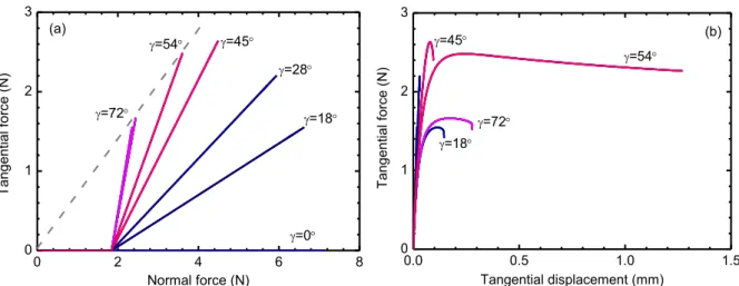
Figure 2.3 Local behaviour of dense sand ( p₀ 800kPa): (a) tangential force versus normal

force; (b) tangential force versus tangential displacement ... 71

Figure 2.4 Total work and plastic work of dense sand ( p₀ 800kPa): (a) total work in macro scale and micro scale during loading, (b) plastic work evolution for various integration directions ... 71

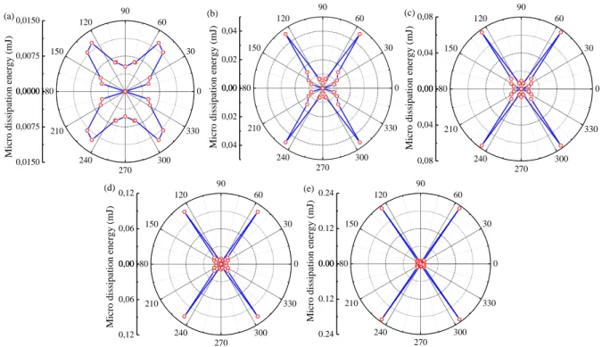
Figure 2.5 Free energy and dissipation energy evolution at the micro scale of dense sand under drained compression (e₀ 0.549, p₀ 800kPa): (a) free energy under isotropic compression, (b) dissipation energy at axial strain 2.14%, (c) dissipation energy at axial strain 4.94%, (d) dissipation energy at axial strain 10.14%, (e) dissipation energy at axial strain 20% ... 72

Figure 2.6 Dissipation energy evolution at the micro scale of loose sand under undrained compression (e₀0.9, p₀ 800kPa): (a) dissipation energy at axial strain 1%, (b) dissipation energy at axial strain 3%, (c) dissipation energy at axial strain 6%, (d) dissipation energy at axial strain 12%, (e) dissipation energy at axial strain 20% 73 Figure 3.1 RVE of unsaturated granular soil as a closed thermodynamic system ... 79

Figure 3.2 Total stresses in a RVE of unsaturated granular soils (figure from Zhang, 2016) . 79 Figure 3.3 Branch vector and distance vector ... 90

Figure 3.4 Performance of the reference hydraulic potential function ... 91

Figure 3.5 Chiba sand: (a) grain size distribution; (b) water retention curve ... 93

Figure 3.6 Critical state of Chiba sand in (a) p q plane and (b)elogp plane ... 95

Figure 3.7 Simulation of the constant water content triaxial compression tests on unsaturated Chiba sand (w10%) ... 96

Figure 3.8 Simulation of the constant water content triaxial compression tests on unsaturated Chiba sand (w17%) ... 97

Figure 4.1 Performances of CPA for dense sand and loose sand under drained and undrained compressions: (a) deviatoric stress versus axial strain, (b) void ratio versus axial strain for dense sand, (c) deviatoric stress versus axial strain for loose sand, (d) deviatoric stress versus mean effective stress for loose sand ... 112 Figure 4.2 Performances of CPPM for dense sand and loose sand under drained and undrained

(14)

strain for dense sand, (c) deviatoric stress versus axial strain for loose sand, (d) deviatoric stress versus mean effective stress for loose sand ... 113 Figure 4.3 Isoerror maps plotted under mixed controls and strain controls: (a) CPA for

drained triaxial test, (b) CPPM for drained triaxial, (c) CPA for undrained triaxial test, (d) CPPM for undrained triaxial test ... 114 Figure 4.4 Biaxial test simulation: (a) meshes and boundary conditions, (b) distribution of

equivalent plastic strain ... 116 Figure 4.5 Biaxial tests by various increments using (a) CPPM, (b) CPA to integrate force-displacement relations ... 117 Figure 4.6 Evolution of interparticle contact forces of the selected element: (a) normal forces

(N), (b) tangential forces (N) ... 117 Figure 4.7 Finite element model of a square footing: (a) equivalent plastic strain of dense sand,

(b) reaction force and vertical displacement of the square footing ... 119 Figure 4.8 Evolution of interparticle contact forces of the selected element: (a) normal forces

(N), (b) tangential forces (N) ... 119 Figure 5.1 Rendulic plane: (a) triaxial probe, (b) strain probe circle ... 130 Figure 5.2 Stress-strain relation with confining pressure of 800kPa: (a) deviatoric stress

versus axial strain of dense sand (e0=0.5), (b) deviatoric stress versus mean

effective pressure of dense sand (e0=0.5), (c) deviatoric stress versus axial strain

of loose sand (e0=0.885), (d) deviatoric stress versus mean effective pressure of

loose sand (e0=0.885) ... 131

Figure 5.3 Second-order work calculated by Piola-Kirchhoff stress and Cauchy stress, and its volumetric part and geometrical parts at point A, B, C and D by Rendulic strain probe ... 132 Figure 5.4 Second-order work calculated by stress-strain and summation of microscale

second-order work at points A, B, C and D by Rendulic strain probe ... 135 Figure 5.5 Force, displacement and force ratio distributions of triaxial drained test at initial

stage and stages A, B, C and D: (a) normal forces on x-y plane, x-z plane and y-z plane (N); (b) tangential forces on x-y plane, x-z plane and y-z plane (N); (c) normal displacements on x-y plane, x-z plane and y-z plane (mm); (d) tangential displacements on x-y plane, x-z plane and y-z plane (mm); (e) force ratios on x-y plane, x-z plane and y-z plane ... 138

(15)

Figure 5.6 Force, displacement and force ratio distributions of triaxial undrained test at initial stage and stages A, B, C and D: (a) normal forces on x-y plane, x-z plane and y-z plane (N); (b) tangential forces on x-y plane, x-z plane and y-z plane (N); (c) normal displacements on x-y plane, x-z plane and y-z plane (mm); (d) tangential displacements on x-y plane, x-z plane and y-z plane (mm); (e) force ratios on x-y plane, x-z plane and y-z plane ... 139 Figure 5.7 Macro and micro second-order work: (a) second-order work calculated by stress-strain and summation of microscale second-order work of dense sand (e0=0.5); (b)

second-order work calculated by stress-strain and summation of microscale second-order work of loose sand (e0=0.885) ... 140

Figure 5.8 Micro second-order work at stages A, B, C and D on x-y plane, x-z plane and y-z plane ... 141 Figure 5.9 Drained biaxial tests of dense sand (e0=0.5): (a) mesh and boundary conditions; (b)

deviatoric plastic strain at stage A; (c) deviatoric plastic strain at stage C; (d) deviatoric plastic strain at stage D ... 143 Figure 5.10 Drained biaxial tests of dense sand (e0=0.5): (a) vertical reaction force versus

vertical displacement; (b) global second-order work ... 144 Figure 5.11 Stress-strain of the selected element of biaxial test during loading (e0=0.5): (a)

deviatoric stress versus axial strain, (b) deviatoric stress versus mean effective pressure ... 144 Figure 5.12 Force, displacement and force ratio distributions at initial stage and stages E, F

and G of selected element of biaxial test: (a) normal forces on x-y plane, x-z plane and y-z plane (N); (b) tangential forces on x-y plane, x-z plane and y-z plane (N); (c) normal displacements on x-y plane, x-z plane and y-z plane (mm); (d) tangential displacements on x-y plane, x-z plane and y-z plane (mm); (e) force ratios on x-y plane, x-z plane and y-z plane ... 146 Figure 5.13 Macro and micro second-order work of selected element during loading and

failure plane of biaxial test (e0=0.5): (a) second-order work calculated by

stress-strain and summation of microscale second-order work; (b-d) micro second-order work at stages E, F and G on x-y plane, x-z plane and y-z plane ... 147 Figure 5.14 Undrained biaxial tests of loose sand (e0=0.885): (a) deviatoric plastic strain at

stage A'; (b) deviatoric plastic strain at stage B'; (c) deviatoric plastic strain at stage C'; (d) deviatoric plastic strain at stage D' ... 148

(16)

Figure 5.15 Biaxial tests of dense sand (e0=0.885): (a) vertical reaction force versus vertical

displacement; (b) global second-order work ... 149 Figure 5.16 Stress-strain of the selected element of biaxial test during loading (e0=0.885): (a)

deviatoric stress versus axial strain, (b) deviatoric stress versus mean effective pressure ... 149 Figure 5.17 Force, displacement and force ratio distributions at initial stage and stages E, F

and G of selected element of biaxial test: (a) normal forces on x-y plane, x-z plane and y-z plane (N); (b) tangential forces on x-y plane, x-z plane and y-z plane (N); (c) normal displacements on x-y plane, x-z plane and y-z plane (mm); (d) tangential displacements on x-y plane, x-z plane and y-z plane (mm); (e) force ratios on x-y plane, x-z plane and y-z plane ... 151 Figure 5.18 Macro and micro second-order work of selected element during loading and

failure plane of biaxial test (e0=0.885): (a) second-order work calculated by

stress-strain and summation of microscale second-order word; (b-d) micro second-order work at stages E, F and G on x-y plane, x-z plane and y-z plane ... 152 Figure 5.19 Direction of strain localisation at the end of biaxial tests: (a) dense sand (e0=0.5)

under drained condition; (b) loose sand (e0=0.885) under undrained condition . 152

Figure 5.20 Force-displacement of biaxial tests with smooth boundaries: (a) dense sand (e0=0.5) under drained condition; (b) loose sand (e0=0.885) under undrained

condition ... 153 Figure 5.21 Drained biaxial tests of dense sand (e0=0.5) with smooth boundary: (a) deviatoric

plastic strain at stage A; (b) deviatoric plastic strain at stage B; (c) deviatoric plastic strain at stage C; (d) deviatoric plastic strain at stage D ... 154 Figure 5.22 Undrained biaxial tests of loose sand (e0=0.885) with smooth boundary:

deviatoric plastic strain and pore pressure at (a) stage A'; (b) stage B'; (c) stage C'; and (d) stage D' ... 154 Figure 5.23 Deviatoric plastic strain and pore water pressure of selected elements of the

undrained biaxial tests with smooth boundary: (a) plastic strain; (b) pore water pressure ... 155 Figure 5.24 Distribution of random initial void ratio of granular assembly: (a) dense; (b) loose ... 156 Figure 5.25 Force-displacement of biaxial tests on dense sand (e0=0.45-0.55): (a) rough

(17)

Figure 5.26 Drained biaxial tests of dense sand (e0=0.45-0.55) with rough boundary: (a)

deviatoric plastic strain at stage A; (b) deviatoric plastic strain at stage B; (c) deviatoric plastic strain at stage C ... 157 Figure 5.27 Drained biaxial tests of dense sand (e0=0.45-0.55) with smooth boundary: (a)

deviatoric plastic strain at stage A; (b) deviatoric plastic strain at stage B; (c) deviatoric plastic strain at stage C ... 158 Figure 5.28 Force-displacement of biaxial tests on loose sand (e0=0.80-0.97): (a) rough

boundary; (b) smooth boundary ... 159 Figure 5.29 Undrained biaxial tests of loose sand (e0=0.80-0.97) with rough boundary:

deviatoric plastic strain and pore pressure at (a) stage A'; (b) stage B'; (c) stage C' ... 159 Figure 5.30 Undrained biaxial tests of loose sand (e0=0.80-0.97) with smooth boundary:

deviatoric plastic strain and pore pressure at (a) stage A'; (b) stage B'; (c) stage C' ... 160 Figure 6.1 Flow chart of explicit finite element analysis based on the ABAQUS/Explicit ... 164 Figure 6.2 Simulations of drained triaxial compression tests using IPP, UMAT and VUMAT ... 165 Figure 6.3 Simulation of biaxial test: (a) mesh and boundary condition (b) distribution of

deviatoric strain ... 166 Figure 6.4 Dimension of the FE model: (a) foundation and (b) square footing area ... 167 Figure 6.5 Settlement of a square footing: (a) total displacement and (b) accumulated

deviatoric shear strain ... 168 Figure 6.6 Force-displacement relation of the square footing ... 168 Figure 6.7 Finite element model of soil and tunnel lining ... 170 Figure 6.8 Distributions of the (a) displacement (m); (b) vertical displacement (m); (c) shear

strain at the end of lining ... 171 Figure 6.9 Ground settlement: (a) Peck’s method and (b) CH model and Peck’s prediction 172 Figure 6.10 Shear strain observed in the experiments on sand by moving a retaining wall: (a)

translation, passive (b) translation, active (c) rotation about the top, passive (d) rotation about the top, active (e) rotation about the toe, passive (f) rotation about the toe, active (figures from Niedostatkiewicz et al., 2010) ... 173

(18)

Figure 6.11 Calibration of the CH micromechanical model (data from Kolymbas and Wu,

1990) ... 174

Figure 6.12 Simulation of the retaining wall: (a) the finite element model and (b) loading modes ... 175

Figure 6.13 Transition, passive ... 176

Figure 6.14 Rotation about bottom, passive ... 176

Figure 6.15 Rotation about top, passive ... 176

Figure 6.16 Transition, active ... 177

Figure 6.17 Rotation about bottom, active ... 177

Figure 6.18 Rotation about top, active ... 177

Figure 6.19 Deformation of a continuum in a Lagrangian (left) and a Eulerian analysis (right) (figure from Qiu et al., 2011) ... 179

Figure 6.20 Particle size distribution of Dog’s bay sand (data from Kuwajima et al., 2009) 180 Figure 6.21 Critical state lines of Dog’s bay sand: (a) elogp plane; (b) p q plane (experimental data from Coop, 1990) ... 180

Figure 6.22 Simulations of drained triaxial compression tests on Dog’s bay sand: (a) deviatoric stress vs axial strain (b) volumetric strain vs axial strain (experimental data from Kuwajima et al., 2009) ... 181

Figure 6.23 Closed-ended pile driven in sand (a) finite element model and (b) base resistance ... 182

Figure 6.24 Finial state of the closed-ended pile: (a) total displacement (b) mean effective stress (c) deviatoric shear strain (d) deviatoric stress ... 183

(19)

LIST OF TABLES

Table 2.1 Parameters used in micromechanical model for Hostun sand ... 70

Table 3.1 Micro-macro relations of energetic quantities ... 86

Table 3.2 Initial condition of constant water content triaxial compression tests on Chiba sand ... 94

Table 3.3 Parameters used in the micromechanical model for Chiba sand ... 95

Table 4.1 Constraint matrices for mixed controls ... 103

Table 4.2 Algorithm for mixed control ... 104

Table 4.3 Implicit integration of macro-micro relation ... 106

Table 4.4 Closest point projection method (CPPM) for local law ... 109

Table 4.5 Cutting-plane algorithm (CPA) for local law ... 110

Table 4.6 Performances of implicit algorithms on triaxial drained and undrained tests ... 113

Table 4.7 Performances of implicit algorithms in biaxial drained test simulations ... 118

Table 4.8 Performances of implicit algorithms in finite element analysis of square footing 118 Table 6.1 Parameters used in the CH micromechanical model for Karlsrule sand ... 174

(20)

LIST OF NOTATIONS AND ABBREVIATIONS

LATIN SYMBOLS

A Second-order fabric tensor T

a First partial derivative of the yield function at inter-particle contacts

T

b First partial derivative of the potential function at inter-particle contacts C Consistent tangential moduli for CPPM

c cth inter-particle contact

D Dilatancy parameter at inter-particle contact

d50 Grain size correspond to 50% pass by mass on the size distribution curve

E Constraint matrices of strain under mixed control

Ec Kinetic energy

e Void ratio

e0 Initial void ratio

c

e Void ratio at critical state

ref

e Reference void ration in critical state line

w

e Void ratio of water

F Deformation tensor in Lagrangian description

F Yield function at inter-particle contact c

f Force at inter-particle contact

ref

f Reference normal force

G Potential function at inter-particle contact

H Hardening variable used in the implementation of CPA c

ij

k Stiffness matrix at the microscale

rR

(21)

pR

k Ratio of plastic stiffness over normal stiffness at inter-particle contact

i

l Branch vector between two contacting particles M The slope of critical state line in p'-q plane

N Number of inter-particle contacts

NP Number of integration points over a unit sphere

p' Mean effective stress

pref Reference mean effective stress

q Deviatoric stress

r Radius of particles

S Constraint matrices of stress under mixed control

s Matric suction

ij

s Nominal stress tensor

Sr Degree of saturation

T Absolute temperature

u Internal energy per unit volume

V Volume of granular assembly

W Work input per unit volume

W2 Global second-order work

2 c

W Particle scale second-order work

2 el

W Elementary scale second-order work p

r

W Plastic work at inter-particle contact induced by tangential force

w Water content

GREEK SYMBOLS

α α th integration point on a unit sphere c

(22)

β Angle in local coordinate (n, s, t)

γ Angle in local coordinate (n, s, t) c

δ Inter-particle displacement at cth contact Δλ Plastic multiplier for both CPPM and CPA

Δ2_λ _{Increment of plastic multiplier for CPPM}

ΔX Loading vector

κ Hardening function in the CH model

λ Compression index in critical state line

λc _{Non-negative plastic multiplier}

μ Standard deviation in Gauss distribution

ε Euler strain tensor q

 Deviatoric strain

ξ (γ, β) Directional density function of homogenization

Π First Piola-Kirchhoff stress tensor

 Dissipation energy increment per unit volume  _{Density of granular soils}

σ Cauchy stress tensor

 Gibbs free energy per unit volume c



 Inter-particle contact friction angle c

d

 Dilatancy angle at inter-particle contact c

p

 Peak friction angle at inter-particle contact c

χ Dissipative force at cth inter-particle contact



_{Helmholtz free energy per unit volume}

w(α) Weight coefficient in αth direction Ω Integration domain in a unit sphere

(23)

ABBREVIATIONS

BBM Barcelona Basic Model

BXD Drained biaxial compression test BXU Undrained biaxial compression test CPA Cutting plane algorithm

CPPPM Closest point projection method DEM Discrete Element Method FEM Finite element method

REV Representative element volume

RTOL Tolerance for mixed control, set to be 10-3

TOL1 Tolerance of yield criterion at inter-particle contacts, set as 10-7

TOL2 Tolerance of residual plastic displacement for CPPM, set as 10-2 TXD Drained triaxial compression test

TXU Undrained triaxial compression test

(24)

GENERAL INTRODUCTION

1. Motivation

Granular materials consist of solid particles with interparticle voids that can be fully or partially filled with fluids. The mechanical behaviour of granular materials is important in many branches of engineering and science, such as in pharmaceutical industry, agriculture, energy, and geotechnical and geophysical applications. Granular soils from clay to rockfill materials (with increasing of grain size) are very typical granular materials and construction fills in engineering practice. Although many efforts have been made to improve our understanding of the behaviour of granular soils, developing more physical and practical methods of geotechnical design is still an open issue.

Based upon continuum mechanics, the finite element method (FEM) has been widely used to solve geotechnical problems, in which constitutive models are required to represent the behaviour of granular soils. Generally, these models are developed based upon classical continuum mechanics using the concept of representative element volume (REV) and some assumptions, such as the critical state theory and/or the dilatancy theory (Rowe, 1962; Schofield and Wroth, 1968). Due to the complexities of granular soils including pressure dependent modulus, loading path dependency, and induced fabric anisotropy etc., many ad

hoc parameters are required to reproduce the behaviour of granular soils by constitutive

models at the macro scale. In this phenomenological modelling, constitutive equations are proposed rather for mathematical fitting than with physics insight.

To circumvent the shortcomings of constitutive models based on continuum mechanics, the discrete element method (DEM) has been used and, in some cases, combined with FEM to solve boundary value problems. In this approach, DEM samples were used to serve as the Gauss integration points in FEM. The applicability of the FEM×DEM approach was well demonstrated by Zhao and Guo (2014), Nguyen et al. (2017), etc. However, the experimental data on particle properties and on their contacts are difficult to obtain precisely. Hence, this method can be only qualitatively used for engineering problems. In addition, the demand of

(25)

computational cost is still an unsolved problem; consequently, the number of particles in one Gauss integration point is very limited even though parallel computing techniques have been used.

Given the limitations of the phenomenological models and the huge computational cost of DEM, constitutive models based on micromechanics have been developed. In this approach, the stress-strain relations are obtained by defining interparticle contact laws and averaging the local variables to obtain the global ones with homogenization techniques. Micromechanical models have proved their efficiency in describing the behaviour of granular soils under various loading conditions with few parameters with physical meanings (Chang and Hicher, 2005; Yin and Chang, 2009; Nicot and Darve, 2005, 2011; Xiong et al., 2017).

From an energy perspective, the thermodynamic principles lead to a generally accepted framework. However, many heuristic models, including the original Cam-Clay model (Schofield and Wroth, 1968), do not satisfy this theory, so one may raise the question: do the micromechanical models satisfy the first and the second laws of the thermodynamic principles? If not, how to construct a thermodynamically consistent micromechanical model? For practical purposes, the micromechanical models should be accurately integrated into a finite element code to analyse boundary value problems. In particular, it is of interest to demonstrate that this numerical method can be widely used in geotechnical engineering practice.

2. Objectives

The overall objective of this thesis is to develop a multiscale approach to describe the behaviour of granular soils in order to solve geotechnical problems. For this purpose, the thesis will focus on the following specific objectives:

First, since the thermodynamic principles represent the general physical laws, it is important to develop the techniques of thermodynamics with internal variables (Houlsby and Puzrin, 2007) for constructing micromechanical models. In doing so, the micromechanical models for granular soils are natural outcomes of both physical and energy conservation models.

(26)

Thermomechanical formulations for constructing micromechanical models for dry and partially saturated granular soils can then be derived and serve as theoretical bases for constructing thermodynamically constrained micromechanical models.

Additionally, numerical techniques for integrating the developed micromechanical models to solve boundary value problems will be discussed and demonstrated. Numerical integration schemes will be proposed to accurately integrate micromechanical models. As an example, the CH model (Chang and Hicher, 2005) will be implemented into a finite element code to fulfil multiscale modelling of geotechnical problems. With this approach, the extent of grain scale instability to granular assembly failure will be investigated. Furthermore, this method will be used to solve some classical geotechnical problems at small and large deformations.

3. Outline of the thesis

This thesis elaborates the objectives presented above in the following chapters:

Chapter 1 reviews the basic theories of micromechanics of granular materials, the developed micromechanical models, and the development of multiscale approaches in geotechnical engineering.

Chapter 2 answers the question: how to construct a thermodynamically consistent micromechanical model for dry granular materials. Thermodynamics with internal variables has been extended to the multiscale approach, based on which a micromechanical model for dry granular soils has been constructed.

Chapter 3 develops the thermomechanical multiscale modelling approach to partially saturated granular soils. A micromechanical model for unsaturated granular soils based on the proposed framework has been constructed.

Chapter 4 focuses on the implicit integration of the micromechanical models based on the static hypothesis through three levels of integration algorithms. The CH model has been selected as an example to be accurately integrated and has been implemented into an implicit finite element code for multiscale modelling of boundary value problems.

(27)

Chapter 5 introduces the capability of the CH model in describing the instability of granular assemblies. Consistent relations for the second-order work at the micro scale, the material point scale and the engineering scale have been obtained. With this method, localised and diffuse failures of granular assemblies have been analysed.

Chapter 6 presents the applications of the CH model in solving geotechnical problems at small and large deformations. Four examples, including a square footing, the excavation of a tunnel, a retaining wall and the installation of a closed-ended displacement pile, have been analysed with an explicit finite element method to demonstrate that micromechanical models can be applied successfully to geotechnical engineering.

Finally, a general conclusion summarizes the work presented in this thesis and discusses potential directions for future development.

(28)

CHAPTER 1 MULTISCALE MODELLING OF GRANULAR

MATERIALS

1.1 Introduction

Granular materials are composed of a large number of grains and voids. To describe the behaviour of granular materials, heuristic models have been constructed based upon classical continuum mechanics (Kolymbas, 2012). In this kind of phenomenological modelling approach, many ad hoc parameters need to be calibrated in order to simulate the complex behaviour of granular materials under a wide range of loading conditions. In comparison, the multiscale modelling approach regards granular materials as assemblies of discrete grains and voids (Chang and Hicher, 2005; Yin and Chang, 2009; Nicot and Darve, 2005, 2011; Radjai et

al., 2017), and thus accounts for more physics. Correspondingly, inter-particle contact laws

have to be defined and localization and averaging operators need to be given, as shown in Figure 1.1 (Cambou et al., 2009, 2016). This chapter begins with recent developments of micromechanics in granular materials, in which the elastic and plastic contact laws, relations between micro-macro variables and the techniques used to construct multiscale models will be discussed. After that, attention is paid to constitutive relations developed on the basis of micromechanics of granular materials. Finally, the multiscale modelling approaches that have been used in solving geotechnical problems will be discussed.

Figure 1.1 General framework of multiscale approach in granular materials (figure from Cambou et al., 2009)

(29)

1.2 Micromechanics of granular materials 1.2.1 Interparticle contact laws

The relations between two contacting particles depend on the characteristics of grains, such as stiffness and geometry. In terms of the grain stiffness, hard grains are such that deformation of the grain itself can be negligible, while soft grains can be deformed with or without time dependency. The geometry of the grain greatly affects the frictional behaviour between particle contacts. Therefore, different interparticle contact laws should be defined for different kinds of granular materials. Among these relations, elastic and plastic local relations for spherical grains have been widely adopted.

1) Elasticity

The expression of the stiffness between two contacting particles due to normal and shear forces can be dated back to Hertz and Mindlin (Mindlin and Deresiewicz, 1953), who considered two contacting elastic bodies as two rigid bodies connected by deformable springs. These springs are distributed in the normal direction to represent normal forces and in the tangential direction to describe shearing forces. For simplicity, the two springs are generally considered as uncoupled from each other. The normal stiffness depends on the normal force and the properties of grains, given as

 

1

c c

n n

k C f  (1.1) where C and α are material parameters, 1

c n

f is the interparticle contact normal force. A

general expression for shear stiffness was suggested as

2 1 tan c c c r r n c c n f k C k f       _  _   (1.2)

where C and β are material constants, ₂ c r

f is the interparticle contact shear force and c



 is the friction angle between grains.

Revised forms of Eqs. (1.1) and (1.2) have been widely adopted in literature. In DEM simulations as well as in the micromechanical models constructed by Nicot and Darve (2005,

(30)

2011), the normal and tangential stiffness are material constants. In comparison, Chang and Hicher (2005) adopted spherical particles to describe granular soils, in which the revised stiffness was adopted

0 2 c c c n n n g f k k G l     _ _   , 0 2 c c c n r r g f k k G l     _ _   (1.3)

where G_g is the elastic modulus of particles and l is the branch length of two contacting

particles, while the reference normal stiffness c₀ n k is given by 2/3 0 12 2 1 c n g g d k G v    _ _    (1.4)

in which d is the particle diameter and vg being the Poisson’s ratio of the grains.

2) Plasticity

A Coulomb type plastic criterion has been extensively adopted to represent the frictional behaviour of granular materials. A general formulation of this type of criterion can be expressed as



    

2 2

 

, c c c c c i s t n i F f   f  f  f   (1.5) in which κ is a function of the interparticle displacement c

i

 . If κ is a constant then Eq. (1.5) reduces to be a pure plastic function, which has been generally applied in DEM simulations (Cundall and Strack, 1979), in the -D model (Nicot and Darve, 2005) and in the H-model (Nicot and Darve, 2011), see also section 1.3. By comparison, the CH model (Chang and Hicher, 2005) and its developing models consider displacement hardening yield criteria for sand, clay and other cohesive granular materials, which will be addressed in detail in section 1.3. Note that for clay, a second compression type plastic criterion is needed (Yin and Chang, 2009; Yin et al., 2009, 2010, 2011, 2013, 2014).

1.2.2 Strain tensors

In classical continuum mechanics, many definitions of a strain tensor can be found in the literature, such as the left or right Cauchy-Green strain tensor, Piola deformation tensor,

(31)

Green-Lagrange strain tensor, Euler-Almansi strain tensor etc. (Bagi, 2006; Cambou et al., 2009, 2016). These tensors are expressed in terms of the translation gradient tensor. In micromechanics of granular materials, strain tensors are defined based on the granular assemblies which can be viewed as a REV. The global deformation of the assembly originates from displacements and rotations of particles. With these micromechanics-based strain tensors, discrete element simulation results can be explained and micromechanical models can be constructed. There are many ways to define strain tensors in terms of the interparticle displacements. Among them, most of the strain tensors were defined based on an equivalent continuum and a best-fit method (Bagi, 2006).

1) Strains based on an equivalent continuum

In these approaches, the granular assembly is replaced by a continuous field through a suitable translation field, which assigns the displacements of particle centres to the equivalent continuum. Strain tensors defined along this line can be found in the work of Bagi (1993, 1996), Kruyt and Rothenburg (1996), Kuhn (1997, 1999), Cambou et al. (2000) and Kruyt (2003).

2) Strains defined from the best-fit methods

In these methods, the deviations between the theoretical displacement field and the actual displacement field should be minimum, hence the obtained displacement field is the best-fit of the actual displacement field. The difference between the strain tensors lies in the consideration of the local displacement field (Bagi, 2006; Cambou et al., 2016). For instance, the displacement of the centres of neighbouring grains was adopted in Cundall and Strack (1979). In contrast the relative displacement at the interparticle contacts was used in Liao et

al. (1997), whereas the relative displacement of the centres of neighbouring particles was

calculated in Cambou (2000).

In this thesis, only the strain tensor conforming to the best-fit type proposed by Liao et al. (1997) will be presented, since it will be used as an assumption in the following chapters. In micromechanics of granular materials, if each particle would move exactly according to a

(32)

uniform translation gradient _ij, then the deformation at contact c would be

c c

i ji j

d  l (1.6)

Since the displacement fields of granular materials are strongly heterogeneous, for a general ij

 we would find that

0

c c

i ji j

d  l  (1.7)

To find a strain tensor ij which is closer to the actual displacement field, the square sum of the deviations in Eq. (1.7) should be the smallest, that is to say







1 min N c c c c i ji j i ji j c Z d  l d  l  



   (1.8) The condition for minimum of Z can be obtained when

0 kl Z   _  (1.9)

Solving Eq.(1.9) leads to

1 1 N N c c c c n m ni i m c c l l



d



l     _   







(1.10) in which n, m and i can be 1, 2 or 3. Defining a fabric tensor as

1 1 1 N c c nm n m c A l l V        



 (1.11)

and combining Eqs. (1.10) and (1.11), the strain tensor proposed by Liao et al. (1997) can be obtained 1 1 N c c ni i m nm c d l A V         



 (1.12)

which states that the strain of a granular assembly is the volumetric summation of interparticle displacements with branch vectors and connection with fabric tensor.

1.2.3 Effective stress tensors

(33)

materials, in particularly in soil mechanics. For dry and fully saturated granular materials, the relation between total stress total

ij

 and effective stress _ij can be generally written as total

ij ij pw

  (1.13) where p is the fluid pressure in fully saturated condition; _w  0 for dry state and 1 for the saturated condition. In both cases, the effective stress _ij has been well established in micromechanics of granular materials, which is equal to the so-called contact stress tensor _ij given by interparticle contact force and branch vector connecting two contact particles. This formulation is also termed as the Love-Weber formula (Love, 1927; Weber, 1966), given as

1 1 N c c ij i j c f l V   



(1.14) in which c i

f is the force at interparticle contacts.

For partially saturated granular materials, the difficulty in using Eq.(1.13) lies in quantifying the coefficient χ. On one hand, it has been found that the parameter χ could not be generally expressed via a function of the degree of saturation, particularly under drying-wetting cyclic loadings (Gens et al., 2006). On the other hand, efforts also have been made to give the definition of the effective stress _ij . From recent results obtained by discrete element simulations, it seems that the Love-Weber formula could not be generally used as an effective stress tensor for unsaturated granular materials. This issue is a focal topic for researchers with interests in partially saturated granular materials (Duriez and Wan, 2016; Chalak et al., 2017).

1.2.4 Fabric tensors

To describe the internal structure of granular materials, fabric tensors have been introduced. Generally, the geometrical information on granular particles and their spatial arrangement can be described by a second-rank tensor. Various definitions of the fabric tensor have been proposed (Satake, 1982; Oda et al., 1985; Santamarina and Cascante, 1996; Kuganenthira et

(34)

classified as contact normal-based, particle orientation-based and void-based tensors (Wang et

al., 2017). The former two types of tensors can be generally expressed as

1 1 2 N k k k N  



 F v v (1.15)

where N is the number of the entities being quantified; the superscript k is the kth entity; k

v

is the directional entity which could be the unit contact normal or the unit particle orientation vector. The void-based fabric tensor was initially proposed by Li and Li (2009) and then developed by Fu and Dafalias (2015) for two-dimensional assemblies. The fabric tensor based on void cell system suggested by Li and Li (2009) can be written as

 

0 1 v N k k k k v v k v E v E N  



 F n n n (1.16) where k

v

is the length of the thk void vector whose direction is k

n ;

 

k v

E n is the directional

distribution of the void vector density; N is the total number of void vectors; _v E is a ₀

normalization factor which can be derived from the statistics theory (Kanatani, 1984; Li and Yu, 2011) and is equal to 2 in 2D space and 4 in 3D space. From these definitions, we can see that the fabric tensor defined in Eq.(1.11) is a revised form of the contact-based fabric tensor and satisfies the unit volume requirement of the thermodynamically consistent fabric tensor (Li and Dafalias, 2015).

Fabric tensors can be decomposed into an isotropic part and a deviatoric part. An isotropic material indicates that the same material response can be obtained if the loading direction is rotated. The deviatoric part, also termed as fabric anisotropy, includes inherent anisotropy and induced anisotropy. The former one refers to an initial anisotropy that is caused by previous loadings, such as the inherent anisotropy of granular soils caused by the gravity, while the latter one is induced by the subsequent loadings.

It has been recognized that the non-coaxial behaviour of granular materials under proportional loading and continuous rotational shearing originates from their fabric anisotropy. Therefore, well considering the evolution of fabric anisotropy is crucial for describing the non-coaxial

(35)

deformation of granular materials. Discrete element simulations have found that the fabric anisotropy tends to reach a steady state even when the inherent anisotropy is different (Fu and Dafalias, 2011; Kruyt, 2012; Zhao and Guo, 2013; Kruyt and Rothenburg, 2014, 2016; Yang and Wu, 2016). According to these findings, Li and Dafalias (2012) extended the classical critical state theory (Schofield and Wroth, 1968) by involving a fabric item, which also reaches a critical value at the classical critical state. In this framework, constitutive models were constructed to simulate the non-coaxial deformation of granular soils (Li and Dafalias, 2012; Gao et al., 2014; Gao and Zhao, 2017).

1.2.5 Averaging and localisation operators

The Love-Weber formula described by Eq. (1.14) has been proved to be a general expression for dry granular materials, it is therefore adopted as an averaging operator for micromechanical models (Chang and Hicher, 2005; Yin and Chang, 2009; Yin et al., 2009, 2010, 2011, 2013, 2014; Nicot and Darve, 2005, 2011; Xiong et al., 2017).

Two types of localisation operators: the kinematic method and the static hypothesis can be generally found in literature (Chang and Hicher, 2005; Nicot and Darve, 2005, 2011; Yin et

al., 2009; Misra and Singh, 2014; Misra and Poorsolhjouy, 2015a; Xiong et al., 2017). The

former one bridges global strains and inter-particle displacements, such as the widely-used expression in Eq.(1.6), based on which micromechanical models were constructed by Nicot and Darve (2005, 2011), Misra and Singh (2014), Xiong et al. (2017). The latter one gives inter-particle incremental forces from incremental global stresses, for instance the one adopted by Chang and Hicher (2005), rewritten as

,

c c c c

i ij n jn i ij n jn

f  l A f  l A (1.17) where A_jn is given in Eq. (1.11). Based on Eq. (1.17), a family of micromechanical models

has been constructed (Chang and Hicher, 2005; Yin and Chang, 2009; Yin et al., 2011, 2013, 2014; Zhao et al., 2017).

(36)

The summation of local quantities over all interparticle contacts can be approximated by directional statistics theory. This theory was first proposed by Kanatani (1984) for directional orientations represented by unit vectors, and then was extended by Li and Yu (2011) for directional vectors in which both magnitude and direction are of significance. The distribution of both orientations and vectors along all directions can be approximated by a probability density function f n

 

. The approximation of the function f n

 

can be obtained by a smooth

function F n

 

, which can be expressed as a polynomial

 

i i ij i j ijk i j k ijkl i j k l

F n  C C n C n n C n n n C n n n n  (1.18)

where n is a unit vector. The integration of the function F n

 

should satisfy

 

1 with

 

0

F d F



  



n n (1.19) where dΩ is an elementary solid angle (Figure 1.2) and Ω represents the unit circle in 2D case and the unit sphere in 3D case. Let n(1)_{, n}(2)_, _{and n}(N)_{be unit vectors representing an}

observed number of N local directional data. An empirical distribution of the contact probability density f (n) is

 



 



1 1 N c c f N   



 n n n (1.20)

where 

 

 is the Dirac delta function defined as

 

, x=0 0, x 0  _{  }



 , which also satisfies the

identity 

 

d 1

   



. f n

 

is nonnegative and automatically satisfies f

 

d 1

  



n . y x z   d sin d d   o

(37)

Eq.(1.18) can be approximated using the polynomial function as

 

_{1 2} ₁ ₂ _{1 2} ₁ ₂ _{1 2} ₁ ₂ 0 0 1 1 1 n n n n i i i i i i i i i i i i i i i i F F n n n D n n D n n n E E     _     _ n (1.21) where E₀ d 



_

, which is equal to 2 in 2D space and 4 in 3D space; the tensor coefficients 1 2 n i i i F and 1 2 n i i i

D can be determined by minimizing the least square error

 

2

min

E F f d







_ n  n _ n (1.22)

The most fundamental quantities of these directional data are their average values. The average of the nth order tensor product, also termed as the moment tensor of order n is given as

 

1 2 1 2 1 2 1 2 1 1 n n n n N c c c i i i i i i i i i i i i c N n n n n n n F n n n d N  _  







n n (1.23)

The directional tensor

1 2 n

i i i

F in Eq. (1.21) can be determined by minimizing the least square

error criteria

 

1 2 1 2 1 2 1 2 1 2 1 2 0 n n n n n n i i i j j j j j j i i i i i i i i i E F n n n d F n n n n n n N F _  _ _ _ _ 



n n (1.24)

where the identity

1 2 1 2 0 1 n n i i i i i i n n n n n n d E _





, which can be explicitly integrated, as expressed by Li and Yu (2011). By substituting the obtained direction tensor

1 2 n

i i i

F from Eq.

(1.24) to Eq. (1.21), we obtain



Fi i1 2 in Di i1 2 in



n ni1 i2 nin Fi i1 2 in2n ni1 i2 nin2 (1.25)

The coefficient tensor

1 2 n

i i i

D can be finally expressed as

 





1 2 2 1 2 1 2 2 1 2 1 2 2 2 ! 1 2 ! n n n n n i i i _n i i i j j j j j j i i i n n D N F n n n n n n n     (1.26)

(38)

2 2 2 , 2 2 1 , 3 2 1 n n n n C D D n        _  _  (1.27) in which n k

C stands for the number of k-combinations of a n-element set. In view of the

symmetry in 1 2 n i i i F and 1 2 n i i i

D , their relation can be expressed as

1 2 n 1 2 n 1 2 n2 n1n

i i i i i i i i i i i

F D F _  _ (1.28)

For direction-dependent vectors with different magnitudes, Li and Yu (2011) gave the form of approximating the directional representative values as

 

m H0 ji₁ i_nn ni₁ i₂ ni_n m G n0



0 jG nji₁ i₁ Gji₁ i_nn ni₁ i₂ ni_n 



M n (1.29)

in which the direction tensors

1 n

ji i

H and

1 n

ji i

G can be determined by minimizing the least

square error

 

min E d      

_

_M n m n _{ } M n m n _   (1.30)

where m n

 

is the directional distribution of a representative vector. The procedure for

solving Eq.(1.30) is the same as for solving Eq.(1.22).

The described directional statistics theory has been widely applied in deriving the stress-force-fabric relations (Rothenburg and Bathurst, 1989; Li and Yu, 2013; He et al., 2017; Wang

et al., 2017), in analysing results of discrete element simulations (Li and Yu, 2011; Li et al.,

2013; Li, 2016), in experimental and numerical quantification of fabric tensors (Yang et al., 2007, 2008; Yang and Wu, 2016; Xie et al., 2017), as well as in constructing micromechanical models (Chang and Hicher, 2005; Yin and Chang, 2009; Nicot and Darve, 2005, 2011; Misra and Singh, 2014, 2015; Misra and Poorsolhjouy, 2015a; Xiong et al., 2017; Zhao et al., 2017).

1.3 Micromechanical models

A variety of multiscale constitutive relations, also termed as micromechanical models, have been proposed based on micromechanics of granular materials. In this section, several typical micromechanical models will be reviewed. Specific attentions will be paid on the CH model

Multiscale modelling of granular soils : from the grain to the structure scale

HAL Id: tel-02124168

https://tel.archives-ouvertes.fr/tel-02124168

Multiscale modelling of granular soils : from the grain to

the structure scale

Chaofa Zhao

To cite this version:

Modélisation multi-échelle des sols granulaires : de

l’échelle des grains aux structures géotechniques

ACKNOWLEDGMENTS

ABSTRACT

RÉSUMÉ

TABLE OF CONTENTS

LIST OF FIGURES









LIST OF TABLES

LIST OF NOTATIONS AND ABBREVIATIONS



GENERAL INTRODUCTION

CHAPTER 1

MULTISCALE MODELLING OF GRANULAR

MATERIALS

 



    

 

























v

 



v

 

 

 

 

 

 

 

 



 







 

 

 



 

 



 



 

 



 





 









 

 

_

_