Contribution to robust and fiabilist optimization : Application to the design of acoustic radio-frequency filters

HAL Id: tel-03098455

https://tel.archives-ouvertes.fr/tel-03098455

HAL is a multi-disciplinary open access archive for the deposit and dissemination of sci-entific research documents, whether they are pub-lished or not. The documents may come from teaching and research institutions in France or abroad, or from public or private research centers.

L’archive ouverte pluridisciplinaire HAL, est destinée au dépôt et à la diffusion de documents scientifiques de niveau recherche, publiés ou non, émanant des établissements d’enseignement et de recherche français ou étrangers, des laboratoires publics ou privés.

filters

François Schott

To cite this version:

François Schott. Contribution to robust and fiabilist optimization : Application to the design of acoustic radio-frequency filters. Vibrations [physics.class-ph]. Université Bourgogne Franche-Comté, 2019. English. �NNT : 2019UBFCA031�. �tel-03098455�

TH `ESE DE DOCTORAT DE L’ ´ETABLISSEMENT UNIVERSIT ´E BOURGOGNE

FRANCHE-COMT ´E

PR ´EPAR ´EE `A L’UNIVERSIT ´E DE TECHNOLOGIE DE

BELFORT-MONTB ´ELIARD

´

Ecole doctorale n°37

Sciences Pour l’Ing´enieur et Microtechniques Doctorat de Sciences pour l’Ing´enieur

par

Franc¸ois

Schott

Contribution to robust and fiabilist optimization

Application to the design of acoustic radio-frequency filters

Th`ese pr´esent´ee et soutenue `a Besan¸con, le 20 d´ecembre 2019

Composition du Jury :

ELMAZRIAOmar Professeur `a l’Universit´e de Lorraine - Institut Jean Lamour-CNRS

Pr´esident du Jury

BIGEON Jean Directeur de recherche CNRS, G-SCOP Rapporteur

IDOUMGHAR Lhassane Professeur `a l’Universit´e de Haute-Alsace - Institut IRIMAS

Rapporteur

BARONthomas Ing´enieur de Recherche, HDR, ENSMM D´epartement Temps-Fr´equence, Institut FEMTO ST, (UMR 6174 CNRS/UFC/ENSMM/UTBM)

Directeur de th`ese

MEYERYann Maˆıtre de Conf´erences HDR, Sorbonne Universit´es, Universit´e de Technologie de Compi`egne, CNRS, UMR 7337 Roberval, centre de recherche Royallieu, CS 60 319, 60203 Compi`egne cedex, France

Codirecteur de th`ese

CHAMORETDominique Maˆıtre de Conf´erences, ICB UMR 6303, CNRS Univ. Bourgogne Franche-Comt´e, UTBM, Belfort, France

Encadrant

SALMONS´ebastien Ing´enieur de recherche, AR-electronique Invit´e

écol e doctoral e sciences pour l ’ingénieur et microtechniques

Universit´e Bourgogne Franche-Comt´e 32, avenue de l’Observatoire

25000 Besan¸con, France

Title: Contribution to robust and fiabilist optimization

Keywords: Optimization, Radio-frequency, Engineering design optimization, Robust optimization, Fiabilist optimization, Surface acoustic wave, SAW filters, MEMS

Abstract:

This thesis aims to develop robust and fiabilist optimiztion means in order to face the future requirements of the radio-frequency (RF) filter market. The goals of this thesis are: to reduce the optimization process timespan, to be able to find a solution that fully satisfies a tough bill of specifications and to reduce failure rate due to manufacturing uncertainties. Several research works has been done to achieve these goals.

During the formulation phase of an engineering design optimization (EDO) process, ambiguities, leading to unsatisfying solutions, could happen. In this case, some phases of the EDO process has to be iterated increasing its timpespan. Therefore, a Framework to properly formulate an optimization problem has been developed. During a run of optimization, for the algorithm to solve the problem according to the designer’s preferences and thus avoid un-satisfying solution, two challenges, among others, have to be faced. The variable challenge is about handling mixed variables with different order of magnitudes while the satisfaction challenge is about properly computing satisfaction. The Normalized Evaluations approach has been developed to face these challenges. The resolution method efficiency strongly relies on the choice of its core element: the algorithm. Hence, the high number of optimization algorithms is a challenge for an optimizer willing to choose the correct algorithm. To face this challenge, a Benchmark, being a tool to assess the algorithm

performance and to be able to select the correct algorithm for a given problem, has been developed. Algorithm efficiency depends on the values given to its parameters, its setting. A common practice is to tune parameters manually which does not guarantee the best performance. A solution to this problem is to perform meta-optimization (MO) which consists in optimizing an algorithm efficiency by tuning its parameters. A MO approach using a benchmark to evaluate settings has been tested. A fiabilist optimization method, taking the uncertainties into account, has to be developed. However, this method has to do so without degrading resolution time, which is usually the case with fiabilist methods. Therefore, a Sparing Fiabilist Optimization method taking uncertainties into account without increasing too much the numerical resolution timespan has been developed.

These methods have been applied to optimize a RF filter, with a tough bill of specifications, for which no fully satisfying solution where found before the thesis. By using the methods developed during this thesis, a determinist solution, not taking uncertainties into account, which fully satisfies the bill of specifications, has been found. Moreover, a fiabilist solution having a 71% success rate has been found. As a conclusion, it appears that optimization methods developed during these thesis where sufficient to face the future requirements of the radio-frequency filter market.

Titre : Contribution to robust and fiabilist optimization

Mots-cl´es : Optimisation, Radio-fr´equence, Optimisation en conception, Optimisation robuste, Optimisation fiabiliste, Onde de surface acoustique, Filtre SAW, MEMS

R´esum´e :

Cette th`ese vise `a d´evelopper des moyens d’optimisation robuste et fiabiliste dans le but de faire face aux besoins du march´e des filtres radio-fr´equence (RF). Les objectifs de cette th`ese sont: r´eduire la dur´ee du processus d’optimisation, ˆetre capable de trouver une solution qui satisfasse compl`etement un cahier des charges difficile et r´eduire le pourcentage de rebut dˆu aux incertitudes de fabrication. Plusieurs travaux de recherche ont ´et´e men´es pour atteindre ces objectifs.

Durant la phase de formulation d’un processus d’optimisation en conception (EDO), des ambigu¨ıt´es, conduisant `a des solutions insatisfaisantes, peuvent survenir. Dans ce cas, certaines phases du processus d’EDO doivent ˆetre it´er´ees augmentant sa dur´ee. Par cons´equent, un cadre pour formuler correctement les probl`emes d’optimisation a ´et´e d´evelopp´e. Durant un run d’optimisation, pour que l’algorithme r´esolve le probl`eme conform´ement aux attentes du concepteur et ainsi ´eviter les solutions insatisfaisantes, deux d´efis, parmi d’autres, doivent ˆetre surmont´es. Le d´efi des variables consiste `a g´erer des variables mixtes ayant des ordres de grandeur diff´erents tandis que le d´efi de la satisfaction consiste `a correctement calculer celle-ci. L’approche par ´evaluations normalis´ees a ´et´ee d´evelopp´ee pour faire face `a ces d´efis. L’efficacit´e de la m´ethode de r´esolution d´epend fortement du choix de son ´el´ement central: l’algorithme. De ce fait, le grand nombre d’algorithmes d’optimisation est un d´efi pour un concepteur souhaitant choisir un algorithme adapt´e. Pour faire face `a ce d´efi, un benchmark, qui est un outil pour ´evaluer la performance d’un

algorithme et ˆetre capable de choisir l’algorithme adapt´e `a un probl`eme, a ´et´e d´evelopp´e. L’efficacit´e d’un algorithme d´epend des valeurs donn´ees `a ses param`etres, son param´etrage. Une pratique commune est de r´egler les param`etres manuellement, ce qui ne garantit pas les meilleures performances. Une solution `

a ce probl`eme est de r´ealiser une m´eta-optimisation (MO) qui consiste `a optimiser l’efficacit´e d’un algorithme en r´eglant son param´etrage. Une approche de MO utilisant un benchmark pour ´evaluer des param´etrages a ´et´e test´ee. Une m´ethode d’optimisation fiabiliste, prenant en compte les incertitudes, doit ˆetre d´evelopp´ee. Cependant, cette m´ethode ne doit pas d´egrader le temps de r´esolution, ce qui est g´en´eralement le cas des m´ethodes fiabilistes. Ainsi, a m´ethode d’optimisation fiabiliste ´econome prenant en compte les incertitudes sans trop augmenter le temps de calcul ont ´et´e d´evelopp´ee.

Ces m´ethodes ont ´et´e appliqu´ees pour optimiser un filtre RF, avec un cahier des charges difficile, pour lequel aucune solution totalement satisfaisante n’avait ´et´e trouv´ee avant la th`ese. En utilisant les m´ethodes d´evelopp´ees durant cette th`ese, une solution d´eterministe, ne prenant pas en compte des incertitudes, respectant totalement le cahier des charges, a ´et´e trouv´ee. De plus, une solution fiabiliste ayant un pourcentage de succ`es de 71% a ´et´e trouv´ee. En conclusion, il apparaˆıt que les m´ethodes d´evelopp´ees durant cette th`ese sont suffisantes pour faire face aux besoins futurs du march´e des filtres radiofr´equences.

Acknowledgments /

Remerciements

Remerciements

Une th`ese ce n’est pas seulement un travail mais aussi un th´esard. Un th´esard qui part `a l’aventure pour environ trois ans. Pour moi, cette aventure commence quand S´ebastien Salmon , ami et ancien patron, d´ecide de me proposer de faire une th`ese au sein de son entreprise, My-OCCS. Aussi, avant de remercier tous ceux qui m’ont aid´e dans cette aventure, je commencerai par ’Merci Patron !’.

Pour d´emarrer une th`ese, encore faut-il un financement et un projet. J’aimerais donc remercier le FEDER pour avoir financ´e, `a travers la bourse FC0001257 - 11002, le projet Smart-Inn dont ma th`ese a fait partie.

Pour qu’une th`ese se passe bien, et pour faire face aux impr´evus de celle-ci, il est fortement conseill´e d’avoir de bons encadrants. Des encadrants qui veillent `a ce que vous gardiez le cap, `a vous former et `a s’assurer que tout va bien. Merci `a Thomas Baron , Yann Meyer , Dominique Chamoret et S´ebastien Salmon pour leur bienveillance, leur p´edagogie et leur pers´ev´erance.

Pour finir une th`ese en beaut´e, le rˆole du jury est primordial. Je tiens donc `a remercier Omar Elmazria , Jean Bigeon et Lhassane Idoumghar pour l’implication et l’ouverture d’esprit avec lesquelles ils ont ´evalu´e mon travail, pour m’avoir aid´e `a prendre du recul par rapport au travail r´ealis´e et pour m’avoir aid´e `a am´eliorer le m´emoire.

Les travaux men´es durant cette th`ese ont ´et´e possibles grˆace `a des collaborations avec diff´erents partenaires. J’en profite pour remercier Florence Bazzaro, Sophie Col-long , Raed Koutta ainsi que les employ´es d’AR-Electronique et de Frec|n|sys pour leur chaleur humaine, leur motivation et le temps qu’ils ont pris pour m’expliquer leurs domaines respectifs.

Une th`ese c’est aussi ´evoluer au sein d’un labo. Je remercie l’ensemble des membres du d´epartement temps-fr´equences pour leur convivialit´e, leur passion communicative pour la recherche et pour ce qu’ils m’ont appris. Un merci tout particulier pour mes coll`egues de bureau, Alex , Arthur , Damien , Guillaume, Justin , Melvin , Mihaela , Stefania et Tung , pour leur bonne humeur, pour l’entraide et pour toutes les discussions (s´erieuses ou non) qu’on a pu avoir. Merci ´egalement `a Bernard , Ch´erita , Nicolas et Val´erie pour ˆetre pass´e r´eguli`erement nous voir et prendre le temps de discuter.

J’ai eu la chance d’ˆetre bien accompagn´e tout au long de cette aventure. Un grand merci aux doctorants du TF, Alex , Alok , Anthony , Arthur , ´Etienne, Falzon , Fa-tima , Gautier , Giacomo, Gr´egoire, Guillaume, Hala , Isha , J´er´emy , K´evin , Melvin , Sabina , Stefania , Tung et Vincent , pour tous les bons moments pass´es en-semble: les midis au RU, pour les soir´ees et sorties (pool party, fˆete de la musique, volley

et basket) et pour les conf´erences, s´eminaires et autres training schools en tous genres. C’est d’ailleurs grˆace aux doctorants du TF que j’ai rejoint l’A’Doc, L’association des jeunes chercheurs de Franche-Comt´e. Je remercie les membres de l’A’Doc et en par-ticulier les membres des bureaux, Alex , Alice, Dj´e, ´Etienne, Gr´egoire, Guillaume, Jason , J´erˆome, Julien , Marie, Nico et Romain , pour les ´ev´enements, pour m’avoir permis de discuter des hauts et des bas d’une th`ese et surtout pour les r´eunions (pas assez s´erieuses pour ˆetre efficaces donc toujours suffisamment peu pour passer un bon moment). La th`ese m’a aussi permis de d´ecouvrir le Bozendo, un art martial au bˆaton long. Merci beaucoup aux Bozendokas de Besan¸con et d’ailleurs, et notamment `a Pierre, Isahia , Sandrine, Titouan , Nico, Elias, Gwen , Marius, Marion , Mathieu , Ed-ward , Aliz´e, Mikhail , Pierre, Raph , JC , Colombe, C´edric, Jean-Marie, L´etitia , Patrice, C´eline, Guillaume, Jean-Seb, Bastien , Cassandre, Sophie, Ch´eima , Gwen et Mathieu , pour leur bonne humeur, pour m’avoir aid´e `a progresser, pour m’avoir fait confiance pour prendre des cours et pour me permettre de pratiquer mon art martial pr´ef´er´e. Merci en particulier `a Marion et `a Pierre pour leur enthousiasme, pour avoir fait vivre le club et pour avoir motiv´e les troupes sur le tamis comme pour sortir.

Cette th`ese, je la dois aussi `a l’UTBM . D´ej`a, parce que c’est grˆace `a l’UTBM que j’ai rencontr´e S´ebastien Salmon qui m’a pris en th`ese. Mais aussi, parce que c’est l’UTBM qui m’a pr´epar´e `a la th`ese et qui a servi de cadre `a celle-ci. C’est pourquoi je souhaite remercier le personnel et les professeurs de l’UTBM ainsi que les ´el`eves , que ce soit ceux avec qui j’ai ´etudi´e ou ceux que j’ai eu la chance d’avoir en cours.

Mais l’UTBM, plus encore qu’une ´ecole, ce sont des UTBoh´emiens, des amis pour la vie. Un tr`es grand merci `a mes amis UTBoh´emiens pour avoir fait passer les ´etudes si vite, pour toutes les soir´ees, week-ends et vacances o`u j’ai pu mettre la th`ese de cˆot´e et m’amuser et pour avoir toujours ´et´e l`a. Parce qu’il n’y aurait pas de Dr Schott sans Mister Keum, merci `a Saoul , Hans, Camille, Tac, Minal , Magne, Iredla , Glion , Soeur , Dygne, Afumer , Skia , Gobelin , Shka , Iki , Nam , Yther , Pik´e, L´erone, Bob, Moaljon , 6 , Mowgly , Zia et Aoline. Merci beaucoup `a Hans et Camille pour avoir relu le m´emoire.

J’ai aussi eu la chance de pouvoir compter sur des amis d’un peu partout. Je tiens `

a remercier mes amis de Besan¸con, de Metz et de Chine. Merci `a Paul , Marie, Julien , P.O., Adri et Monc pour avoir gard´e le contact, pour les soir´ees `a Metz et `a Nancy et pour les vir´ees dans les Vosges. Merci `a Th´eo, Akira , Vincent et Eduard pour les week-ends retrouvailles, les souvenirs de Chine et les soir´ees parisiennes. Merci `a Shakit , Andy , Kent et toute l’´equipe de SZAA pour tous les bons moments que j’ai pass´es avec eux durant mon stage en Chine lequel m’a pr´epar´e `a affronter les difficult´es d’une th`ese. Merci `a Groom , Emilia et Sonia pour les bons moments que j’ai pass´es `a Besan¸con avec eux.

Pour conclure, et il est temps, merci `a ma famille, Tonio, M’man , P’pa , Jean-Jacques, Amy , Nathalie, Hubert , Jules, Marie, Baptiste, Dora , Audrey , Louis, L´eopold , Augustine, Lucie, Cl´ement , Ir`ene, Xavier et aussi `a Caroline et Pierre-´

etienne. `A ceux qui m’ont vu grandir, `a ceux `a qui je dois tant, `a ceux qui ont toujours ´

et´e l`a, `a ceux dont on se sent toujours proche malgr´e le temps et la distance, merci pour tout et un peu pour le reste aussi.

vii

Acknowledgments

A Ph.D. thesis is not only at work, but also a Ph.D. Student. A student going on a journey for approximately three years. For me, this journey began with S´ebastien Salmon , a friend and former boss of mine, proposing me a thesis at his own company, My-OCCS. Also, before thanking all whom helped on this journey, I would begin with ’Thanks Boss!’. To begin a thesis, one must find a subvention and a project. I would therefore thank the ERDF for subventioning, through the grant FC0001257 - 11002, the project Smart-Inn which my thesis is part of.

For a theist to go well, and to be able to face the unexpected events related to it, it is strongly advised to have good supervisors. Supervisors whom ensure you stay the course, whom form you and assure everything is going well. Thank you to Thomas Baron , Yann Meyer , Dominique Chamoret and S´ebastien Salmon , for their kindness, their pedagogy and their perseverance.

For a thesis to finish on a high note, the jury is key. I want to thank Omar Elmazria , Jean Bigeon and Lhassane Idoumghar , for the involvement and open mind they have while evaluating my work, for helping me to step back from my work and for helping me to improve the manuscript.

The research works done during this thesis have been possible thanks to collabo-rations with different partners. I’m taking this opportunity to thank Florence Baz-zaro, Sophie Collong , Raed Koutta and also the employee of AR-Electronique and Frec|n|sys for their human warmth, their motivation and the time they spent explaining me their research fields.

A thesis it’s also being part of a Lab. I thank all the members of the Time and Frequency department for their friendliness, their communicative passion for research and for all they taught me. A special thank for my office colleagues, Alex , Arthur , Damien , Guillaume, Justin , Melvin , Mihaela , Stefania and Tung , for their good mood, for the assistance and for the talkings (serious or not) that we had. Thank you also to Bernard , Ch´erita , Nicolas and Val´erie, for regularly visiting the office and spending time to talk.

I have been lucky to be well accompanied all along my journey. A big thank to the TF Ph.D. Students, Alex , Alok , Anthony , Arthur , ´Etienne, Falzon , Fatima , Gautier , Giacomo, Gr´egoire, Guillaume, Hala , Isha , J´er´emy , K´evin , Melvin , Sabina , Stefania , Tung and Vincent , for all the good times we had together: The lunch at the CROUS, the evenings and the go-outs (pool party, music festival, volley and basket) and for all the conferences, seminars and training schools of any kind.

As a matter of fact, it is thanks to the TF Ph.D. students that I joined the A’Doc, the association of the young researchers of Franche-Comt´e. I thank the A’Doc members and in particular the members of the boards, Alex , Alice, Dj´e, ´Etienne, Gr´egoire, Guillaume, Jason , J´erˆome, Julien , Marie, Nico and Romain , for the events, for being here to talk about the ups and downs of a thesis and most of all for the meetings (not serious enough to be efficient and so always not serious enough for having a good time).

The thesis also provides me the opportunity to start practicing the Bozendo, a martial art using a long staff. Thanks a lot to the Bozendokas of Besan¸con and else-where, notably to Pierre, Isahia , Sandrine, Titouan , Nico, Elias, Gwen , Marius,

Marion , Mathieu , Edward , Aliz´e, Mikhail , Pierre, Raph , JC , Colombe, C´edric, Jean-Marie, L´etitia , Patrice, C´eline, Guillaume, Jean-Seb, Bastien , Cassan-dre, Sophie, Ch´eima , Gwen and Mathieu , for their good mood, for helping me to progress, for entrusting me giving class and for giving me the opportunity to practice my favorite martial art. Thank you in particular to Marion , and Pierre, for their enthusi-asm, for carrying the club and for motivating people on the tatami and to go out.

This thesis, I also owe it to the UTBM . Firstly, because it is thanks to the UTBM that I meet S´ebastien Salmon proposing me this opportunity. But also, because the UTBM prepared me to the thesis and provided the framework for it. That’s why I would like to thank the staff and the teachers of UTBM and also the students, both the ones I studied with and the ones I had the chance to have in class.

But UTBM, more than a university, it is UTBohemians, friends for life. A very big thank to my UTBohemian friends for making studies going so fast, for all the evening, weekends and holidays helping me to move the thesis aside to have fun and for always being here. As there shall not be a Dr Schott without a Mister Keum, thank you to Saoul , Hans, Camille, Tac, Minal , Magne, Iredla , Glion , Soeur , Dygne, Afumer , Skia , Gobelin , Shka , Iki , Nam , Yther , Pik´e, L´erone, Bob, Moaljon , 6 , Mowgly , Zia and Aoline. Thanks a lot to Hans and Camille for proofreading this manuscript.

I also have the chance to have friends all around that I can count on. I want to thank my friends of Besan¸con, Metz and China . Thank you to Paul , Marie, Julien , P.O., Adri and Monc, for keeping in touch, for the evenings in Metz and Nancy and for the trips in the Vosges. Thank you to Th´eo, Akira , Vincent and Eduard , for the reunion weekends, for the memories from China and of the Paris nights. Thank you to Shakit , Andy , Kent and all the SZAA staff , for all the good times I had with you during my internship in China, which prepared me for the difficulties I faced during my thesis. Thank you to Groom , Emilia and Sonia , for the good times I had with them in Besan¸con.

To conclude, and it is time, Thank you to my family, Tonio, Ma’ , Pa’ , Jean-Jacques, Amy , Nathalie, Hubert , Jules, Marie, Baptiste, Dora , Audrey , Louis, L´eopold , Augustine, Lucie, Cl´ement , Ir`ene, Xavier and also to Caroline and Pierre-´etienne. To those who see me growing, to those whom I owe so much, to those who always been here, to those whom one always feels closer to no matter the time and the distance, thank you for everything and a little for the rest also.

Contents

1.5 Robustness and Fiability . . . 32

1.6 Conclusion . . . 34

2 A framework to formulate engineering design optimization problems 37 2.1 Introduction . . . 38

2.2 Overview of the proposed framework . . . 38

2.3 Interviews in detail . . . 41

2.4 Conclusion . . . 46

3 The normalized evaluations approach 47 3.1 Introduction . . . 48

3.2 NE approach overview . . . 49

3.3 Variables challenge . . . 51

3.4 Satisfaction challenge . . . 53

3.5 Results and discussion . . . 57

3.6 Conclusion . . . 58

4 A Benchmark for Meta-heuristic, Single-Objective, Continuous Opti-mization Algorithm 61 4.1 Introduction . . . 62

4.2 Architecture of the proposed benchmark . . . 63

4.3 Results of a run . . . 68

4.4 Optimization case result and sub-results . . . 73

4.5 Global score computation . . . 75

4.6 Scoring method analysis through algorithms testing . . . 79

4.7 Conclusion . . . 88

5 Meta-optimization by design of experiment on benchmark used to tune PSO parameters 91 5.1 Introduction . . . 92

5.2 Meta-optimization approach linked elements . . . 93

5.3 Design of experiment . . . 95

5.4 Results and discussion . . . 96

5.5 Conclusion . . . 103

6 Sparing fiabilist optimization 107 6.1 Introduction . . . 108

6.2 Statistical evaluation . . . 109

6.3 Sparing fiabilist optimization method . . . 113

6.4 Sparing fiabilist optimization test method . . . 114

6.5 Results and discussion . . . 117

6.6 Conclusion . . . 125

7 SAW filter optimization 127 7.1 Introduction . . . 128

7.2 SAW filter engineering . . . 129

7.3 Formulation of the SAW filter optimization problem . . . 136

7.4 A method to solve the SAW filter optimization problem . . . 140

7.5 Solving of the SAW filter optimization problem . . . 143

7.6 Conclusion . . . 150

Conclusion 153 References 161 A Appendix 183 A.1 Thematics board . . . 184

A.2 Questionnaire . . . 186

A.3 Optimization bill of specifications . . . 194

A.4 Bound handling techniques . . . 195

A.5 Functions details . . . 197

A.6 Results and Scores computation attached notes . . . 202

A.7 Algorithms detail . . . 205

CONTENTS xi

A.9 Highly constrained problems . . . 212 A.10 Landscape analysis . . . 215

Introduction

Social-economic context

In microelectromechanical systems (MEMS) industry, nine macro-economic megatrends, which will affect our present and future, have been reported in [1]. Those megatrends are: smart automotive, mobile phone, fifth generation cellular network technology (5G), hyperscale data centers, augmented reality/virtual reality, artificial intelligence/machine learning, voice processing, health-care and industry 4.0. They are increasing the demand for MEMS. This market should reach $82B by 2023 [1]. When 5G will arrive, there will also be an increasing need for radio-frequency (RF) filters. The radio-frequency micro-electromechanical systems (RF MEMS) will have the highest growth of the overall MEMS market. According to [1], ’Driven by the complexities associated with the move to 5G and the higher number of bands it brings, there is an increasing demand for RF filters in 4G/5G, making RF MEMS the largest-growing MEMS segment. This market will soar from US$2.3B in 2017 to US$15B in 2023 ’. To develop telecommunication systems for professional, public and strategic applications, such as radar, frequency sources for very high frequencies (VHF: 30–300 MHz) and ultra high frequencies (UHF: 300–3000 MHz) RF bands are needed. The telecommunication market covers several applications requir-ing an accurate selection of frequencies. To face the specifications of these applications in terms of compacity and energy consumption, surface acoustic wave (SAW) RF filters are widely used [2]. For instance, 80% of passive filters used in the emission and reception part of mobile phones are SAW filters.

Radio-frequency filters: Context of this application

do-main

The RF devices are used for signal processing in radio-frequency bandwidth, which consists in analyzing, modifying and synthesizing RF signals. They include RF filters, which are used to filter the signal. A signal is a physical phenomenon which can be used to transmit information [3]. By opposition to signal, noise can be defined as a physical phenomenon polluting signal’s information [4]. Signal is often described as a phenomenon evolving through time [2] and can be expressed into the frequency domain by using Fourier or Laplace transformation [5]. In a general meaning, signal filtering consists in modifying the signal properties depending on frequencies-based criteria [2]. This thesis focuses on frequency filtering consisting in filtering signal in order to keep frequencies in a given bandwidth.

In order to face the telecommunication and internet of things (IoT) markets needs, improving RF filter specifications is essential. The SAW filters and the bulk acoustic wave (BAW) filters technologies can be used for RF filtering. In agreement with research partners, it has been decided that research in optimization will be focused on SAW filters

cases. According to [6], SAW is better than BAW for applications under 1GHz. Moreover, according to [6]: ’The trend in SAW is to improve performance beyond established limits. Higher process complexity is acceptable if the benefit is large enough, if it allows shrinking size, increase yield or save cost in other ways.’.

A SAW filter is a MEMS device, with two ports, which could be represented as a four-poles system. This device uses a piezo-electric substrate to propagate an acoustic wave and metallic inter-digited transducers (IDT) to transform an electrical signal into an acoustic wave and back. The signal response of this device could be expressed through different matrices, notably impedance and admittance ones.

In the sixties, White and Voltmer [7] have proven that IDT could be used for exciting and detecting SAW. In the seventies, IDT were mostly used in military applications, such as radars. In the eighties, SAW filters, developed thanks to prior decade innovations, were massively used in color televisions. In the nineties, to face mobile phone market needs, such as energy consumption reduction, researches on the RF components have been prolific. Currently, the SAW filters are part of the RF market which is about US$5B.

The RF filter sizing will impact its specifications. The product sizing is a stage of the product engineering process where the values of the design parameters are defined. Currently, the RF filter sizing is done by RF experts solely using their knowledge. The RF experts could be helped in this task by using engineering design optimization (EDO).

Engineering design optimization:

Context of this

re-search domain

Engineering design optimization (EDO) [8] aims to optimize product specifications by tuning the design parameters. It is performed during the sizing phase of the design process. To solve an EDO problem, optimization algorithms are more and more often used. In this case, the designer is likely to be helped by an expert in optimization whom will be refereed as an optimizer.

To solve an EDO problem, the designer, helped by the optimizer, thoroughly for-mulates the problem. The designer provides information such as the design parameters to tune or how to evaluate a design from its specifications. With these informations, the optimizer implements the problem in an optimization engine [9]. The optimization engine will numerical solve the problem by using a resolution method, whose core is the optimiza-tion algorithm. The algorithm solves the problem by testing different values. Its goal is to find a sizing with satisfying specifications.

In order to have a better understanding of the work presented in this manuscript, here is a brief history of EDO:

ˆ 18th century: Newton–Raphson’s method to find a local minimum by using derivates. ˆ 19th century: Euler-Lagrange’s works lead to variation computation [10] and to

Lagrange’s multipliers method able to solve constrained problems.

ˆ 40-50’s: Invention of linear programming technics [11] making the transition to mod-ern algorithms. They are mainly used for military and economic applications. ˆ 70’s: First optimization applied to engineering problems. It is the beginning of EDO.

3

ˆ 80’s: Emergence of meta-heuristic methods [12]. A meta-heuristic algorithm is the generalization (meta) of a specialized (heuristic) algorithm. The first generation meta-heuristic algorithms is based on the generalization of the mechanisms of the heuristic algorithms.

ˆ 90’s: Emergence of the second generation of meta-heuristic algorithms [12]. This generation of algorithms is inspired by optimization mechanisms which can be found in nature.

ˆ 2000-2010: The number of second generation meta-heuristic algorithms explodes [12, 13]. Benchmarks [14, 15], which are tools to measure the algorithms performance, are published [13].

Thesis context

Passive RF components are currently limited in terms of specifications by several factors. The main ones are: an incomplete knowledge of the properties of some materials, the technological limits and the physical limits of available materials. To face the future requirements of the RF filter markets, solutions to the previously mentioned limits has to be found. In this context, different organizations have decided to make a scientific partnership: AR Electronique, Digital Surf, My-OCCS, Snowray, Freq|n|Sys, and FEMTO-ST. This partnership, created through the FEDER project SMART-INN1, aims to innovate in the field of RF components through different collaborations.

One of these collaborations aims to develop new passive RF devices with an op-timal design. To achieve such a task, robust and fiabilist optimization solutions suited to SMART-INN problematic should be developed. Hence, it has been decided to start this thesis, which goal is to develop optimization methods to meet the partners needs in optimization. These methods are meant to face three challenges:

ˆ Rapidity, which is how fast the optimization problem is solved. Currently, sizing a RF filter can last up to two weeks for an experienced designer. One of this thesis goal is to reduce this delay to a few days.

ˆ Efficiency, which is how good the specifications of the product are. Currently, when the bill of specifications is tough, even an experienced designer does not always find a sizing respecting all the required specifications. Another goal of this thesis is to find a solution fully satisfying the bill of specifications, even if it is a tough one. ˆ Profitability, which is how affordable the product is. Currently, some designs have

a high failure rate due to manufacturing uncertainties. The last goal of this thesis is to reduce this rate to a few percent by taking the manufacturing uncertainties into account during the sizing phase. In order to do so, the optimization process should lead to the selection of a reliable design.

To face these three challenges, five research works have been done:

1_{Syst`emes `a base de MAt´eriaux de Rupture, principes et outils Technologiques Innovants pour les}

Nouveaux composants passifs acousto-´electriques pour les t´el´ecommunications, les syst`emes radiofr´equences embarqu´es et le traitement du signal du futur (SMART-INN)

ˆ The Framework: how to properly formulate an optimization problem.

ˆ The Normalized Evaluations Approach: how to solve an optimization problem ac-cording to the designer’s expectations.

ˆ The Benchmark: how to assess the performances of algorithms to be able to select the correct one for a given problem.

ˆ The Meta-Optimization: how to tune the parameters of an algorithm for it to be as efficient as possible.

ˆ The Sparing Fiabilist Optimization: how to take uncertainties into account without increasing too much the numerical resolution timespan.

Organization of the thesis

This document is structured by chapters. The first one is a state-of-the-art of optimization. It is followed by five chapters presenting the research works developed during this thesis. The final chapter, application to radio-frequency, describes the optimization of a SAW filter.

In chapter 1, an optimization state-of-the-art is performed. This chapter introduces information required to appreciate the work developed in other chapters. First, what EDO is and how an EDO process is conducted will be introduced. Then, the main elements of an EDO problem, variables, objectives, constraints and evaluation tools, will be ex-plained. The EDO resolution and the algorithms used for this task will be detailed. This introduction will be concluded by two important notions: robustness and fiability.

In chapter 2, the framework developed to properly formulate an optimization prob-lem is presented. This framework is based on interviews during which the optimizer asks questions to the designer. The optimizer is guided in this task by a questionnaire and a thematic board. The designer’s answers are noted to fill in an optimization bill of specifi-cations. Though it has not been tested yet, this framework is proposed to the community. In chapter 3, a normalized evaluations approach designed to solve an optimization problem according to the designer’s expectations, is presented. This approach uses a nor-malized variables intermediate space to ease the algorithm work. In addition, an advanced solution evaluation method is used by the algorithm to properly assess solutions. The approach has been compared to a classical evaluation method on an industrial problem.

In chapter 4, a benchmark, which is a tool to assess the algorithms performance, is proposed. This benchmark, inspired by the CEC one, aims to improve some aspects of algorithms evaluation. With the proposed benchmark, several stopping criteria are used and several scores are computed thanks to normalization and aggregation means. Several algorithms, commonly used in EDO, have been tested with the proposed benchmark to see if the results obtained are confirmed by literature.

In chapter 5, a meta-optimization approach, which improves the efficiency of an algorithm by tuning its parameters, is presented. This meta-optimization approach uses a design of experiment to the find the values of the parameters optimizing the main score of the benchmark for the algorithm tested. These values have been tested both on the benchmark developed in this thesis and on an industrial problem. The results are compared

5

to the ones obtained by using the values defined by an expert in optimization and by other meta-optimization approaches.

In chapter 6, a sparing fiabilist method, which aims to take the uncertainties into account without increasing too much the numerical resolution timespan, is presented. This method is based on both statistical fiabilistic evaluations and deterministic evaluations. The solution used for the algorithms’ global search mechanisms are evaluated in a fiabilist way whereas other solutions are evaluated in a determinist way. The proposed fiabilist evaluation method has been tested on an uncertain version of the benchmark developed in this thesis. The results obtained by the proposed method have been compared to ones obtained by two other fiabilist approaches.

In chapter 7, how to optimize a RF filter, using methods developed in this thesis, is detailed. After an introduction to the RF domain, how to apply previous chapters works to a practical case is explained. The test problem has been solved with and without considering uncertainties.

Finally, the conclusion: summarizes the main results, discusses how they respond to challenges, what are the current limits and what are the prospects.

Acronyms

Table 1: Acronyms

AI Artificial Intelligence

BAW Bulk Acoustic Wave

BBOB Black-Box Optimization Benchmarking

BHT Bound Handling Techniques

BIM Boundary Integral Method

CEC Congress on Evolutionary Computation

CMA Covariance Matrix Adaptation

CMAES Covariance Matrix Adaptation Evolution Strategy

COCO Comparing Continuous Optimizers

CoSyMA Composants et Syst`emes Micro-Acoustiques

DMS Double Mode SAW

DoE Design of Experiment

EDO Engineering Design Optimization

FEM Finite Element Method

FEs Function Evaluations

FO Fiabilist Optimization

FSR Feasible Space Ratio

GA Genetic Algorithm

GECCO Genetic and Evolutionary Computation Conference

IDT Inter-Digited Transducers

IEF Inpedence Elements Filter

IoT Internet of Things

LCRF Longitudinally Coupled Resonator Filter MEMS Microelectromechanical Systems

MO Meta-optimization

MOO Multi-Objective Optimization

NE Normalized Evaluations

OBS Optimization Bill of Specifications OFTS Objective-Function Test Suite

OIA Observation-Interpretation-Aggregation

PC Principal Components

PCA Principal Component Analysis

PSO Particle Swarm Optimization

RCTS Real-Case Test Suite

RBDO Reliability-Based Design Optimization

RF Radio-Frequency

SA Simulated Annealing

SAW Surface Acoustic Wave

SFO Sparing Fiabilit Optimization

SMART-INN Syst`emes `a base de MAt´eriaux de Rupture, principes et outils Technologiques Innovants pour les Nouveaux composants passifs acousto-´electriques pour les t´el´ecommunications, les syst`emes radiofr´equences embarqu´es et le traitement du signal du futur

SNR Signal-to-Noise-Ratio

7

TS Test Suite

UHF Ultra High Frequencies

VHF Very High Frequencies

WHO World Health Organization

Notations

Many notations are used in the following manuscript and sometimes one is close to another either in writing or in meaning. To ensure a good understanding of the content, all these notations are specified in table 2.

Table 2: Notations Optimization Objective F Objective-functions vector f A single objective-function No Number of objective Variable X Variables vector

Xmin The vector of the lower bounds of the variables Xmax The vector of the upper bounds of the variables

x A single variable

xmin The lower bound of a continuous variable xmax The upper bound of a continuous variable s The scale of a discrete variable

l The length of the scale of a discrete variable xi The i-th element of the scale of a discrete variable

D Dimension/Number of variables of an optimization problem

d Index for dimension

S Search space

Constraint G Inequality constraints vector

g A single inequality constraint Ng Number of inequality constraints H Equality constraints vector h A single equality constraint Nh Number of equality constraint

λ A Lagrange multiplier

Advanced notions ∆ Vector of the uncertainties of the variables δ A random uncertainties vector

N The normal distribution law X A confidence limit percentage FSR Feasible space ratio

9

Variable related Z Normalized variables vector

z A single normalized variable

Y Bounded normalized variables vector y A single bounded normalized variable

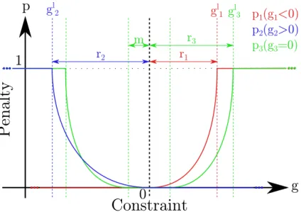
Penalties computation gl The limit value of an inequality constraint gr The reference value of an inequality constraint hr The reference value of an equality constraint hm The error margin of an equality constraint

P The penalties vector

p A single penalty

P The overall penalty

Nj The number of penalties

Bonuses computation

B The bonuses vector

b A single bonus

B The overall bonus

Nb The number of bonuses

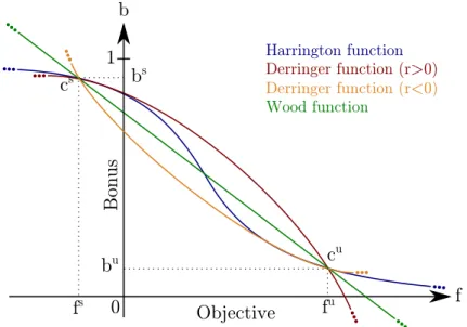
Ci The i-th correspondence point used for a bonus computation fr The objective function value range

fs Satisfying objective value bs Satisfying bonus value

cs Satisfying correspondence point fu Un-satisfying objective value bu Un-satisfying bonus value

cu Un-satisfying correspondence point b( f ) Bonus-function

s The satisfaction

Benchmark General notions

FEs The number of allowed Function Evaluations to solve an optimization problem (stopping criteria)

MaxFEs The ’Maximum Function Evaluations’ coefficient (MaxFEs) is used to adjust FEs.

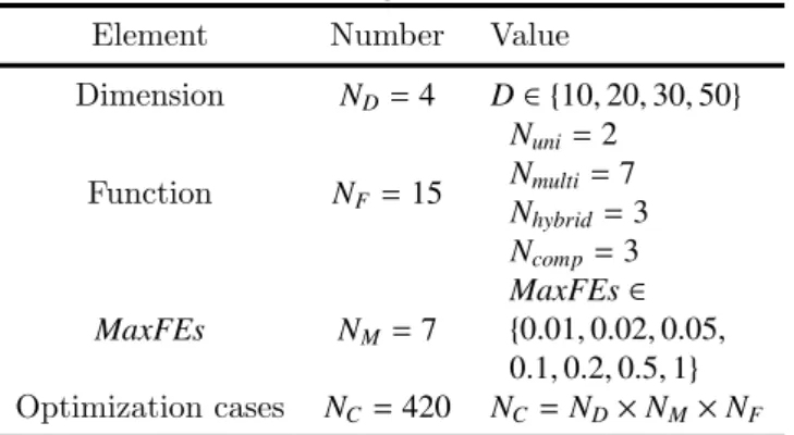
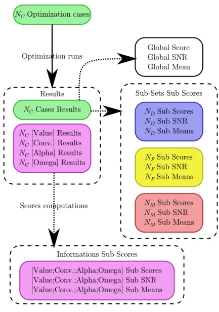
Number of elements ND Number of dimensionality used in the benchmark NF Number of test functions used in the benchmark NM Number of MaxFEs used in the benchmark NC Number of optimization cases of the benchmark NT Number of runs of an optimization case

NR Total number of runs

Functions details

Nuni Number of uni-modal functions used by the benchmark Nmulti Number of multi-modal functions used by the benchmark Nhybrid Number of hybrid functions used by the benchmark Ncomposite Number of composite functions used by the benchmark

Runs

VG Gross value obtain by the algorithm at the end of a run

EG Gross number of evaluations made by the algorithm at the end of a run VN Normalized value of the run

EN Normalized number of evaluations of the run RR Run Result based on the aggregation of VN and EN

Function details fmin Minimum of the objective function fmax Maximum of the objective function

fem Allowed error margin of the objective function

Case results and sub-results RC A case result

RA A case alpha sub-result RO A case omega sub-result RV A case value sub-result RK A case convergence sub-result

Case’s sets of values R_R Set of run results of an optimization case RV Set of value sub-results of an optimization case RE Set of evaluations sub-results of an optimization case

Normalization and aggregation operators ΥE Normalization operator for the gross number of evaluations ΥV Normalization operator for the gross value

A_R Aggregation operator used to compute run result

A_V Aggregation operator used to compute a case value sub-result A_K Aggregation operator used to compute a case convergence sub-result A_A Aggregation operator used to compute a case alpha sub-result A_O Aggregation operator used to compute a case omega sub-result A_C Aggregation operator used to compute a case result

A_M Aggregation operator over MaxFEs A_F Aggregation operator over functions A_D Aggregation operator over dimensions

11

Normalization and aggregation: support V Values/results vector to aggregate

w Normalized weights for values/results to aggregate W Raw weights for values/results to aggregate µI Mean of I, a set of values/results

σI Standard deviation of I, a set of values/results

d Dimensions index

f Functions index

m MaxFEs index

Global score computation

R_Cd f m Case result for dimension d, function f and MaxFEs m Rd f_M MaxFE s intermediate results for dimension d and function f Rd_F Function intermediate results for dimension d

Meta-optimization SNR Signal-to-noise ratio

y A DoE test result

PSO

t Iteration number

v The velocity of a particle

pbest The personal best position of a particle gbest The global best position of all particles

r A random number

c1 The cognition parameter c2 The social parameter ω The inertia of particles itmax Maximal number of iterations Wmin Minimal inertia

Wmax Maximal inertia

vmin The lower bound of random initial velocity given to a particle vmax The upper bound of random initial velocity given to a particle Vfactor The coefficient to compute initial speed bounds

N Population size

R Population radius

Rv Radius threshold value

Rt Number of iteration inside the radius to stop

Sparing fiabilist optimization Fiability general notions

A Uncertain area

sδ The satisfaction of a single daughter evaluation

s∆ The set of the satisfactions of the daughters evaluations

σ Standard deviation P Probability of an event

Sampling size equation notation

n Sampling size

t Margin coefficient deduced from ’c’

c Confidence limit

p Supposed proportion of the elements validating the test e Error margin on the measure

RF RF general notions Vφ Phase velocity λ Wavelength k2 Coupling factor v0 Velocity in substrate v_m Velocity in electrode f Frequency

f0 The center frequency

DMS design parameters

h Electrodes thickness

w Electrodes aperture

a/p Ratio of an electrode width over electrodes mechanical period p Electrodes Mechanical period

l Gap length

n Number of transducers in an element

Filter specifications

Ψ Insertion loss

T Transfer function

R_a Ripples amplitude R_n Number of ripples

Pas Pass band

Rej Rejection band

Φ Group delay

Unclassified

α, β, γ Used for intermediate computations inside an equation

1

Optimization

Contents

1.1 Positioning . . . 14

1.1.1 Engineering Design Opimization in design process . . . 14 1.1.2 EDO process conduction . . . 14 1.1.3 Concept of an EDO process . . . 17

1.2 Problem Formulation . . . 19

1.2.1 Definition of the optimization problem . . . 19 1.2.2 Variables . . . 19 1.2.3 Objective function . . . 20 1.2.4 Constraints . . . 21

1.3 Run of optimization . . . 21

1.3.1 Workflow of an optimization run . . . 22 1.3.2 Evaluations and iterations . . . 23 1.3.3 Stopping criteria . . . 24 1.3.4 Run review . . . 25

1.4 Optimization algorithms . . . 26

1.4.1 Optimization algorithms overview . . . 26 1.4.2 The algorithms used in this thesis . . . 28 1.4.3 Focus on: PSO . . . 30

1.5 Robustness and Fiability . . . 32

1.5.1 Robustness . . . 32 1.5.2 Uncertainties . . . 33 1.5.3 Fiability . . . 34

1.6 Conclusion . . . 34

This chapter intends to introduce the branch of optimization considered in this thesis so that the research works developed in the following chapters could be understood and appreciated. This branch of optimization, the Engineering Design Optimization (EDO), is positioned and presented in section 1.1. EDO consist in finding the best solution to a design problem, which as to be formulated as explained in section 1.2. Once the EDO problem formulated, the expert in optimization could set a resolution method to numerically solve the problem. A single numerical resolution of an EDO problem, a run, is described in section 1.3. The core element of this resolution method is the optimization algorithm, which is introduced in section 1.4. To face this thesis challenge, the resolution method robustness and fiability, defined in section 1.5, should be improved.

1.1/

Positioning

Optimization is a word used in different contexts with multiple meanings. From EDO perspective, optimization consists in creating or designing a product for it to satisfy human needs a much as possible [8]. However, to understand how EDO is performed, one must be aware of the fact that EDO is a branch of ’numerical optimization’ which is a branch of applied mathematics. Indeed, as numerical optimization consists in finding the best solutions (maximizing or minimizing) for a given problem [9], EDO relies on mathematical tools. However, there is a gap between EDO optimization means, which are applied-oriented, and numerical optimization ones, which are theoretical-oriented [16].

In order to define the context in which EDO is performed, section 1.1.1 will posi-tioned EDO into the design process. The EDO could be done by different means which are defined in section 1.1.2. By using optimization algorithm to solve EDO, the EDO process could be decomposed into three phases detailed in section 1.1.3.

1.1.1/ Engineering Design Opimization in design process

From the different modelings of the engineering process which exists [17], the one from Ulrich & Eppinger [18] will be used to position the EDO process into the design one, which is done in figure 1.1. As depicted, the EDO process is used to performed the detailed design step of the design process, in the case of a sub-product. The EDO process, as it is done in a late design step of a low-level product, is performed through a highly specific design step. In higher product levels, an optimization process will either be a combinatorial optimization problem [19] aiming to define product architecture or a large-scale optimization problem [20] aiming to size several sub-product at a time. Both those scenario, which require specific methods, are out of this thesis spectrum. EDO is often done manually and is time consuming, requiring at least 50% of design life cycle [8]. The timespan of this phase, which depends on the method used to conduct EDO, should be reduced to match the rapidity challenge of this thesis.

1.1.2/ EDO process conduction

Several approaches could be used to conduct the EDO process. They are more or less advised depending on the extensiveness and complexity of the the problem to solve. The extensiveness is the amount of information defining the problem while the complexity is how complex the relation between those elements are. Problem extensiveness and

com-1.1. POSITIONING 15 Requirements Statement Early-stage Design Architectural Design Detailed Design Super Product (f.i.: Smart-phone) Requirements Statement Early-stage Design Architectural Design Detailed Design Product (f.i.: RF module) Requirements Statement Early-stage Design Architectural Design

EDO

Figure 1.1: EDO process positionning into the design process - Inspired by [21]

plexity can be estimated from table 1.1. This table, which is inspired by the one from [8], presents the EDO problem classifications that makes sense with regards of the problem faced in this thesis. For each classification, the problem could be classified in a group. These groups will influence problem extensiveness and complexity. The different classifi-cation presented in this table relies on variables, constraints, objectives and environment properties. Variables, which are detailed in sub-section 1.2.2, are the independent product parameters which can be updated to improve the design of a product. Constraints, which are detailed in sub-section 1.2.4, are the constraints the solution to the optimization prob-lem should fulfill to be accepted. The objectives, which are detailed in sub-section 1.2.3, are the product specifications which need to be minimized or maximized. The environment is the additional properties and information of the problem to solve.

Figure 1.2 positions the different EDO approaches with regards to the problem extensiveness and complexity. For instance, for a problem with a low-extensiveness and a low-complexity an analytic approach is advised.

Different approaches are presented by figure 1.2. When a new technical fields arise, no knowledge about it is available. Thus, problem are complex and extensive leading designer to try random design, which is the ’Randomness’ approach. With experience some knowledge will be gathered, and designer will be able to test hypotheses such as the influence of structures or design parameters, which corresponds to medium complexity low extensiveness problem. By doing so designer will perfom optimization by a ’Design of Experiment’ approach [8]. Thanks to the knowledge acquired from these experiements, designer will develop an expertise. This expertise, will enable designer to solve complex problem. This holds as long as the extensiveness is not too high, in which case too many phenomenum should be considered at a time. By using its expertise to optimize a product, a designer is performing an ’expert-based’ approach [8] which could relies on expert rules or Knowledge based systems [8]. For an experience designer to go further,

Table 1.1: EDO problem classifications - inspired by [8]

Classification base Values Problem kind

Variables Number ≤ 10 Low-extensiveness > 10 High-extensiveness Nature Continuous Discrete Mixed High-complexity Constraints

Existence Un-constrained Low-complexity Constrained

Type In-equality Low-complexity Equality High-complexity Linearity Linear Non-linear High-complexity Separability Separable Non-separable High-complexity Objectives Number

1 Low-extensiveness & Low-complexity [2, 10] Low-extensiveness & High-complexity > 10 High-extensiveness & High-complexity

Modality Uni-modal Low-complexity Multi-modal High-complexity Linearity Linear Low-complexity

Non-linear High-complexity Continuity Continuous

Discontinuous High-complexity

Environment

Uncertainties Determinist Low-complexity Fiabilist High-complexity Search space Known

Unknown High-complexity

it should be helped by advanced computation means. First, by using an ’Algorithmic’ approach [8] to face high extensiveness problem, in which case an algorithm is used to find an optimal solution. This approach requires the designer to have enough experience of its fields to set the optimization problem to solve. Second, by ’Neuronal Network’ approach [22, 23] to face medium complexity and medium extensiveness problem. In this approach, a neuronal network is trained and used to find an optimal solution. The neuronal network efficiency will depends on the quality of designs and indications the designer could provide to train it. Finally, some aspects of the design might be studied enough to model them as low extensiveness and low complexity problems. In this case, these aspects could be optimized by ’Analytic’ approach [24, 25], in which case the optimization problem is fully mathematically formulated and solved analytically.

EDO problems are usually solved by an expert-based approach, however the use of algorithms for design optimization is gaining popularity [8]. Indeed, it partially automates the optimization process and allows a better search for the best design. This approach matches with the extensiveness and complexity of the problems to solve in this thesis.

Therefore, this thesis will be restricted to the EDO problem resolution through the algorithmic approach. By using it, the designer will ask an expert in optimization for assistance. This expert, defined as optimizer in this thesis, is in charge of conducting the

1.1. POSITIONING 17

Easy

Problem ComplexProblem

Extensive Problem Hard Problem E x te n s iv e n e s s Complexity

Expert-based

Design of

Experiment

Algorithmic

Randomness

Neuronal

Network

Analytic

Figure 1.2: The engineering design optimization approaches for the different problems -Based on [8]

optimization process to find a solution satisfying the designer’s requirements.

1.1.3/ Concept of an EDO process

The EDO process, being a process of the design process, is introduced in this sub-section. An EDO process, represented in figure 1.3, can be decomposed into three main steps as in [9].

ˆ Formulation:

The formulation phase, detailed in section 1.2, is the phase during which the optimization problem to solve is defined. During this phase, four elements should be defined: the variables, the objectives, the constraints and the evaluation. This phase is performed by interviews between the designer and the optimizer. During this phase, the problem should be defined leaving the fewest amount of ambiguities [21] as possible.

Validated solution D ig

Figure 1.3: The EDO process

The resolution phase is the phase during which an optimization method is set and used to solve the problem. The resolution method is composed of: a bounds handling technique [26], some stopping criteria [9], an optimization algorithm [13] and its setting [27], some eventual simulation tools [9] and an optimization engine [9]. As this thesis is considering optimization from the perspective of engineering sciences and not applied mathematics, in-formation related to computer science such as software, programming languages or library used to develop the optimization engine won’t be detailed in this manuscript. For infor-mation, the optimization engine used in this thesis has been fully developed by F. Schott and S. Salmon in C# programming language without using already existing optimization library. The core element of the solving method is the optimization algorithm. The solving method and the optimization problem are the two elements forming an optimization case. This case will be run to find a solution to the optimization problem. A run, developed in section 1.3, is a single numerical handling of an optimization case.

ˆ Validation:

During the validation phase, the designer decides whether the solution obtained through optimization is validated or not. This phase could be decomposed into several sub-steps. First, the internal verification during which the optimizer validates or not the design. Then, the external verification during which the designer validate or not the design, based on optimization results. Finally, the additional tests during which designer validates or not the solutions based on additional analysis. These analysis are made to test some product specifications that could not be included in the optimization problem, for instance in the case where computing these specifications require to use model too costly in terms of computation time.

1.2. PROBLEM FORMULATION 19

1.2/

Problem Formulation

This section will present the first phase of the EDO process, the formulation, which consists in formulating the engineering problem to be solved as an optimization problem following the classical mathematical formulation. In this phase, several hypothesis and choices are made such as: what will be optimized, what design parameters should be chosen as variables or what requirements should be met. As explained by [28], the early stages of a project are the ones influencing the most the final results. Thus, by analogy, the formulation phase, developed in chapter 2, is surely of importance and should not be neglected.

At the end of the formulation phase, the EDO problem is formulated according to a classical mathematical formulation, which is defined in sub-section 1.2.1. This mathe-matical formulation has a fixed structure that relies on different types of elements detailed in the following sub-sections. The variables, from which objectives and constraints are computed, are presented in sub-section 1.2.2. The objectives, which are to be minimized or maximized, are presented in sub-section 1.2.3. The constraints, which are restricting the problem to satisfying solutions, are presented in sub-section 1.2.4.

1.2.1/ Definition of the optimization problem

From a mathematical point of view, an optimization problem can be formulated as the D-dimensional minimization problem defined in equation 1.1. In this equation, D, the dimension of the problem is the number of design variables X. The vector of objective-functions, F is to be minimized, with respect of the constraints, G and H. The space of possible values for the variables, commonly known as the search space, is noted S.

(P)                        minX∈S ∈ F(X) G(X) ≤ 0 H(X)= 0 X= (x₁, · · · , xD) (1.1) 1.2.2/ Variables

The variables X= (x1, · · · , xD) ∈ S are the independent product parameters which can be updated to improve the design of a product. An optimization problem involves different kinds of variables: continuous or discrete variables. Continuous ones can take any value in a range defined by a lower and an upper bounds (min and max) as follows:

X= (x1, · · · , xD) ∈ S ⇔                      x1∈ [xmin₁ , xmax₁ ] x2∈ [xmin₂ , xmax₂ ] · · · xD∈ [xmin_D , xmax_D ] (1.2)

X= (x₁, · · · , xD) ∈ S ⇔                        x1∈ s1 = n x1₁, x2₁, · · · , xl1 1 o x2∈ s2 = n x1₂, x2₂, · · · , xl2 2 o · · · xD∈ sD= n x1_D, x2_D, · · · , xlD D o (1.3)

Two notions related to the variables are still to be specified: the accuracy and the uncertainty. The accuracy is the expected precision of the solution. The accuracy of the variables can be used as stopping criterion during the run of an optimization prob-lem. The uncertainty corresponds to the manufacturing uncertainty on the variable. The uncertainties are used to perform fiabilist optimization, presented in chapter 6.

1.2.3/ Objective function

In EDO, the objectives, F, are the product specifications which need to be minimized or maximized. By convention an optimization problem consists in minimizing objective-functions, as illustrated in equation 1.1.

ˆ Single-Objective optimization: In this case, the vector of objectives F(X) is composed of a single scalar function which will be noted f .

ˆ Multi-Objective Optimization: Some real-world problems need to achieve sev-eral objectives: Multi-objective Optimization (MOO). In this case, the objective function is a vector defined as follows: F(X)= ( f1(X), f2(X), · · · , fNo(X)) where No is the number of objectives.

As explained by [29], different techniques could be used to deal with multi-objective problem. A classification of criteria optimization approaches, including multi-objective optimization ones, is presented by [30]. In this classification, fifteen multi-objective methods are listed. These methods are first classified in three categories: Pareto, Outranking and Aggregation. Pareto methods, meant to produce a Pareto front [9], pro-vide multiple Pareto-optimal solutions. On the other hand, outranking methods produce solutions ranked according to their dominance over other solutions, according to objectives values. These two categories are not suitable to find a single solution, which is a com-promise between objectives and constraints. Therefore, only aggregation methods, which aims to find a solution making a compromise between objectives and constraints, will be considered. Three methods are mentioned by both [30] and [29]:

ˆ The scalarization method (or weighted-sum method) [9, 29]: This method incorpo-rates multi-objective functions into a scalar fitness function.

ˆ The ε-Constraint method [31]: This approach aims to minimize one objective, say fi(X), subject to the additional constraint fj(x) < εj.

ˆ The goal programming method [32]: Goal programming is a preference-based clas-sical method for solving multi-objective optimization problems [33].

This thesis will focus on single-objective problems. Indeed, after discussion with the Smart-Inn partners, for the SAW filter design problems considered in this thesis,

1.3. RUN OF OPTIMIZATION 21

the main difficulty is to respect the constraints linked to the bills of specifications which are considered tough. Therefore, the problems will be formulated so that specifications are used to produce highly constrained single-objective problems. However, the methods developed in this thesis are designed to face both single-objective and multi-objectives problems.

1.2.4/ Constraints

In optimization, constraints are meant to restrict the search for acceptable solutions. A solution could be considered unacceptable for several reasons, such as not respecting some physics rules or being inadequate with the specifications. The part of the search space where solutions are acceptable is usually referred as the feasible search space. In a classi-cal optimization problem given by equation 1.1, several types of constraint can be distin-guished:

ˆ G which are the inequality constraints; gi refereed to the i-th inequality constraint. ˆ H which are the equality constraints; hi refereed to the i-th equality constraint. ˆ [Xmin_{, X}max_{] which are the lower and upper bounds, as specified in equation 1.2;}

[xmin_i , xmax_i ] refereed to the bounds of the i-th variable.

Several constraints handling techniques exist. Some of the most common techniques are based on penalties. They are either direct, if they are added to the objective-function, or indirect, if they are substituted to the objective-function. Penalties can be fixed values or functions. An usual constraint handling technique is the Lagrange multiplier, detailed in sub-section 1.2.1. Other constraints handling techniques such as the constraints relaxation one [34] and the constraints propagation one [35] focus on how to avoid constrained part of the search space. The constraints relaxation technique uses the constraints formulation to reduce the space search. The constraints ordering technique requires that the problem is solved by a decision tree in which constraints are added one by one at each step.

When the feasible space is highly reduced by constraints, the optimization problem is highly constrained. On this kind of problems, previously described techniques are not always efficient. In this case, other techniques should be used, such as the constraints satisfaction problem ones [36] or the water-fall objective function one [37]. These tech-niques often require the constraints to be ranked in order to be taken into account one after another. Constraints are ranked according to their relative importance, how difficult they are to respect and how flexible they can be.

1.3/

Run of optimization

A run of optimization is a single numerical resolution of an optimization problem. During a run, an optimization algorithm will try to find the optimal solution by searching the value of the variables which maximizes the satisfaction. The algorithm will solve the problem through iterations in which one or several evaluations are made. Historically, the evaluation of a solution simply consists in computing the objective function f from the vector of design variables X. However, in an EDO context, the evaluation process might

be more complex. First, the objective and the constraints might be computed through co-simulation [8]. In this case, the co-simulations could be black-boxes [38]. Secondly, objectives and constraints might be handled through different techniques [10, 39].

In this case, the algorithm does not directly optimize the result of a mathemat-ical objective-function but determines a ’satisfaction’. A satisfaction is a target-value indicating the satisfaction of a designer towards a solution. This satisfaction need to be maximized by the algorithm to obtain the best solution regarding the criteria fixed by the designer.

The satisfaction combines objectives and constraints thanks to a method chosen by the optimizer and set according to the designer expectations. The concept of satisfaction is a generalization of the performance concept introduced in the observation-interpretation-aggregation (OIA) method [21]. The satisfaction will be detailed in chapter 3.

During the formulation phase, the designer should detail how the solution must be evaluated. Several kinds of element should be carefully described: the evaluation tools, the indicators and the satisfaction-related information. The evaluation tools are elements such as the numerical simulation, the analytic model or the computation techniques used during the evaluation process. For each evaluation tool, the designer should explain to the optimizer how to use it. Inputs, outputs, settings, mandatory data files should be discussed. Indicators are information computed during evaluation used to evaluate the product. Satisfaction information are information used to compute the satisfaction of the designer from objectives and constraints.

A run of optimization is an iterative process that could be explained by a workflow, as in sub-section 1.3.1. This process relies on a core element, the algorithm, which per-forms one or several evaluations at each iteration. The evaluation and iteration concepts are presented in sub-section 1.3.2. A run of optimization will iterate evaluations until a stopping criterion is reached. Stopping criteria topic is explored in sub-section 1.3.3. Once stopped, how well a run of optimization was could be evaluated. Hence, how to evaluate a run will be presented in sub-section 1.3.4.

1.3.1/ Workflow of an optimization run

In the case of non-determinist approaches, the workflow of an optimization is summa-rized by figure 1.4. First, the variable are initialized. This can be achieved through different means, for instance randomly [40]. Then, iterations, during which one or sev-eral evaluations are made, are performed. An evaluation corresponds to the succession of the following steps: the variables serve as input for evaluation tools; the evaluation tools computes objectives and constraints; objectives and constraints are used to compute satisfaction. The satisfactions obtained by the evaluations will be used by an algorithm to choose new solutions to evaluate. Which solutions an algorithm will choose to evaluate depends on its setting which is the set of values given to its parameters. In a theoretical context, the evaluation tools will be mathematical functions while in a real case context, the evaluation tools often are numerical models. Finally, evaluations are made until the algorithm reaches a convergence criterion. In this case the algorithm is stopped and the best solution found is the run value.