HAL Id: hal-00301280
https://hal.archives-ouvertes.fr/hal-00301280
Submitted on 16 Oct 2003HAL is a multi-disciplinary open access
archive for the deposit and dissemination of sci-entific research documents, whether they are pub-lished or not. The documents may come from teaching and research institutions in France or abroad, or from public or private research centers.
L’archive ouverte pluridisciplinaire HAL, est destinée au dépôt et à la diffusion de documents scientifiques de niveau recherche, publiés ou non, émanant des établissements d’enseignement et de recherche français ou étrangers, des laboratoires publics ou privés.
Quantification of topographic venting of boundary layer
air to the free troposphere
S. Henne, M. Furger, S. Nyeki, M. Steinbacher, B. Neininger, S. F. J. de
Wekker, J. Dommen, N. Spichtinger, A. Stohl, André Prévôt
To cite this version:
S. Henne, M. Furger, S. Nyeki, M. Steinbacher, B. Neininger, et al.. Quantification of topographic venting of boundary layer air to the free troposphere. Atmospheric Chemistry and Physics Discussions, European Geosciences Union, 2003, 3 (5), pp.5205-5236. �hal-00301280�
ACPD
3, 5205–5236, 2003 Topographic venting S. Henne et al. Title Page Abstract Introduction Conclusions References Tables Figures J I J I Back CloseFull Screen / Esc
Print Version Interactive Discussion
© EGU 2003 Atmos. Chem. Phys. Discuss., 3, 5205–5236, 2003
www.atmos-chem-phys.org/acpd/3/5205/ © European Geosciences Union 2003
Atmospheric Chemistry and Physics Discussions
Quantification of topographic venting of
boundary layer air to the free troposphere
S. Henne1, M. Furger1, S. Nyeki1, 2, M. Steinbacher1, B. Neininger3, S. F. J. de Wekker1, ?, J. Dommen1, N. Spichtinger4, A. Stohl4, †, and A. S. H. Pr ´ev ˆot1 1
Paul Scherrer Institut, Villigen, Switzerland
2
University of Essex, Colchester Essex, UK
3
MetAir AG, Illnau, Switzerland
4
Lehrstuhl f ¨ur Bioklimatologie und Immissionsforschung, Technical University of Munich, Freising, Germany
?
Current affiliation: Pacific Northwest National Laboratory, Richland, Washington, USA
†Current affiliation: NOAA Aeronomy Laboratory, Boulder, Colorado, USA
Received: 21 August 2003 – Accepted: 25 September 2003 – Published: 16 October 2003 Correspondence to: A. S. H. Pr ´ev ˆot ([email protected])
ACPD
3, 5205–5236, 2003 Topographic venting S. Henne et al. Title Page Abstract Introduction Conclusions References Tables Figures J I J I Back CloseFull Screen / Esc
Print Version Interactive Discussion
© EGU 2003
Abstract
Net vertical air mass export by thermally driven flows from the atmospheric boundary layer (ABL) to the free troposphere (FT) above deep Alpine valleys was investigated. The vertical export of pollutants above mountainous terrain is presently poorly repre-sented in global chemistry transport models (GCTMs) and needs to be quantified. Air
5
mass budgets were calculated using aircraft observations obtained in deep Alpine val-leys. The results show that on average 3 times the valley air mass is exported vertically per day under fair weather conditions. During daytime the type of valleys investigated in this study can act as an efficient “air pump” that transports pollutants upward. The slope wind system within the valley plays an important role in redistributing pollutants.
Nitro-10
gen oxide emissions in mountainous regions are efficiently injected into the FT. This enhances their ozone production efficiency and thus influences tropospheric pollution budgets. Once lifted to the FT above the Alps pollutants are transported horizontally by the synoptic flow and are subject to European pollution export. Forward trajectory stud-ies show that under fair weather conditions two major pathways for air masses above
15
the Alps dominate. Air masses moving north are mixed throughout the whole tropo-spheric column and further transported eastward towards Asia. Air masses moving south descend within the subtropical high pressure system above the Mediterranean.
1. Introduction
Nitrogen oxides (NOx= NO2+ NO) and volatile organic compounds (VOC) govern
20
ozone production in the troposphere (Seinfeld and Pandis,1998). Most anthropogenic and biogenic emissions of NOx and VOCs take place in the ABL. The ozone produc-tion efficiency, which is the number of O3 molecules produced by each NOx molecule consumed (Lin et al.,1988), is enhanced by transport to the FT (Seinfeld and Pandis, 1998). Once the air mass has left the ABL, dry deposition of NOxand O3ceases and
25
tro-ACPD
3, 5205–5236, 2003 Topographic venting S. Henne et al. Title Page Abstract Introduction Conclusions References Tables Figures J I J I Back CloseFull Screen / Esc
Print Version Interactive Discussion
© EGU 2003 posphere with increasing altitude the reaction of NO with O3is decelerated. Therefore
the photostationary state of the O3− NOx cycle is shifted to a higher NO/NO2 ratio. In addition peroxyacetyl nitrate (PAN) can act as a reservoir species for NO2 at lower temperatures. The lower the concentration of NO2the more OH radicals react with hy-drocarbons and therefore enhance ozone production (as long as NO > 10 − 30 pptv).
5
Mixing ABL air with FT air, which contains considerable background concentrations of methane and carbon monoxide, leads to a higher hydrocarbon to NOxratio and there-fore again to higher O3production efficiencies.
Therefore, the export of O3 precursors from the ABL to the FT is a crucial compo-nent of the total tropospheric ozone budget. Exchange between the ABL and the FT
10
occurs by processes ranging from synoptic systems, squall lines, deep and shallow cu-mulus and dry convection down to turbulence (Fiedler,1982). Of these, only synoptic systems are resolved in GCTMs, with typical horizontal grid resolutions of ∼ 5◦× 5◦, whereas all other processes have to be parameterized. Vertical transport by deep, moist convection has been quantified in the last two decades (Cotton et al.,1995) and
15
is parameterized in GCTMs (Jacob et al.,1997). Its influence on global O3 budgets, however, is still under debate (Lelieveld and Crutzen,1994). Parameterizations of dry, shallow convection in GCTMs assume ABL mixing, and hold for flat and homogeneous terrain. Above complex terrain (mountainous or coastal), however, thermal wind sys-tems in the range of 0.1 to 100 km develop due to differential heating or cooling of
20
the Earth’s surface during clear sky and strong radiation conditions with weak synoptic forcing (fair weather). Export of trace gases from the ABL in complex terrain to the FT occurs through gaps in the ABL inversion (Kossmann et al.,1999), called topographic venting in the following. Once in the FT, pollutants might be re-circulated regionally on a time scale of a few days (Millan et al.,2002;Tyson and D’Abreton,1998). Elevated
25
layers in the FT are frequently observed (McKendry and Lundgren,2000;Newell et al., 1999), indicating long-range transport of ABL constituents. Entrainment of elevated pollution layers into the ABL leads to increased surface pollutant concentrations at re-mote sites (Berkowitz et al.,2000).
ACPD
3, 5205–5236, 2003 Topographic venting S. Henne et al. Title Page Abstract Introduction Conclusions References Tables Figures J I J I Back CloseFull Screen / Esc
Print Version Interactive Discussion
© EGU 2003 This paper investigates the mechanism of topographic venting within deep Alpine
valleys. Air mass export from the ABL to the FT is quantified by means of air mass budgets. Pollutant export and ozone chemistry will be discussed in a forthcoming pa-per.
2. Measurements and methods
5
2.1. Experimental setup
The VOTALP (Vertical ozone transport in the Alps) (Wotawa and Kromp-Kolb,2000) and CHAPOP (Characterization of high Alpine pollution plumes) field campaigns took place in the Mesolcina and Leventina valleys in the southern Swiss Alps Fig.1. The Leventina valley leads to the San Gottardo road tunnel and the Mesolcina valley to the
10
San Bernardino road tunnel. Steep slopes (slope angle between 20◦ and 25◦), small floor width (0.3 km to 1.0 km) and large depth (1.5 km to 2.0 km) are characteristic of both valleys. Major transalpine traffic routes within the Mesolcina and Leventina valley (∼500 (Mesolcina) and ∼4500 (Leventina) trucks per working day) represent a substantial NOx source at the valley floor of approximately 1 and 10 kg (N) km−1 d−1,
15
respectively.
The measurement setup of the VOTALP Mesolcina study is described in detail by Furger et al.(2000). During the CHAPOP Leventina experiment multiple aircraft were used to investigate the structure and chemical composition of the valley’s atmosphere. On three flight days (26 - 28 August 2001) a small research aircraft (Neininger et al.,
20
2001) operated by the Swiss MetAir acquired meteorological, chemical and aerosol parameters by flying cross sections within the valley (thick black lines in Fig.1). The MERLIN IV research aircraft (Meteo France) flew a box grid pattern at an altitude of 3–4 km a.s.l., measuring parameters similar to the MetAir aircraft. The FALCON re-search aircraft of the German Aerospace Center (DLR) carried a nadir-pointing aerosol
25
struc-ACPD
3, 5205–5236, 2003 Topographic venting S. Henne et al. Title Page Abstract Introduction Conclusions References Tables Figures J I J I Back CloseFull Screen / Esc
Print Version Interactive Discussion
© EGU 2003 ture, ABL development, and aerosol distribution. Radiosondes measuring atmospheric
pressure, temperature, humidity, and wind (ZEEMETTM Mark II MICROSONDE) were launched in the center of the valley. Continuous measurements of standard chemical and meteorological surface parameters were conducted during five weeks (August and September 2001) at three sites, including formaldehyde and detailed VOC analysis.
5
Meteorological data was gathered at two additional sites at the valley’s north-eastern slope. A sodar wind profiling system (Remtech, PA2) was situated at the north-eastern crest of the Leventina valley (Monte Matro, 2172 m a.s.l., eastern side of lidar transect c in Fig.1) and acquired three-dimensional flow data up to 1 km above ground level. 2.2. Mass budget
10
We conducted air mass budget calculations for thermal airflow in the Mesolcina and Leventina valley to quantify vertical air mass export to the FT during daytime, fair weather conditions. Differential heating within a mountainous environment results in up-valley airflow parallel to the valley floor during the day (valley breeze). At the valley sidewalls, up-slope winds prevail (Whiteman, 2000), potentially penetrating the ABL
15
inversion and resulting in export of polluted ABL air.
Vertical wind velocities in thermal updrafts or slope flows can be as high as a few meters per second. However, they are also often spatially and temporally intermittent. Estimating the vertical mass flux out of a valley atmosphere due to slope winds and ver-tical updrafts by direct measurements of the verver-tical wind velocity is therefore a difficult
20
task. In this work we use an indirect method to determine the vertical mass export from the ABL within the valley breeze system to the FT as a residual of horizontal flow measurements.
For budget calculation purposes, a valley segment is composed of a minimum of three open interfaces, two vertical cross-sections within the main valley and a
horizon-25
tal lid. Additional flow into or out of tributary valleys FT has to be considered. Due to conservation of mass, the net vertical mass flux Fz is governed by the convergence of the horizontal mass fluxes Fy,out − Fy,i n, FT and the change of the valley breeze layer
ACPD
3, 5205–5236, 2003 Topographic venting S. Henne et al. Title Page Abstract Introduction Conclusions References Tables Figures J I J I Back CloseFull Screen / Esc
Print Version Interactive Discussion
© EGU 2003 air mass with time FV BL
Fz = Fy,out − Fy,i n+ FT − FV BL. (1)
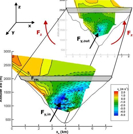
Figure2shows an example of the air flow in the Leventina valley in two cross sections across the valley. Note that up-valley flow is indicated by negative sign and that no tributary valleys are present. Two contrary motions contribute to the net vertical mass
5
flux. During daytime, strong upward motion occurs within the slope wind layer which is only partly balanced by sinking motion in the valley center. Mass balance closure is primarily obtained by the horizontal valley breeze flow.
The flow in the slope wind layer depends on the energy input to this layer by the sensible heat flux at the slope surface, atmospheric stability and the slope angle. The
10
larger the sensible heat flux at the slope surface, the stronger the temperature di ffer-ences between the valley center and the slope layer, providing the driving force for the slope winds. On the other hand, vertical motion is damped with increasing atmospheric stability. But near neutral stability prevents the generation of an organized slope wind due to enhanced turbulent vertical mixing (Vergeiner and Dreiseitl, 1987). Maximal
15
upward flow was simulated in atmospheric numerical models for intermediate atmo-spheric stability (Atkinson and Shahub,1994).
Mass budget calculations of the daytime valley breeze system have to date only been conducted for the broad Alpine Inn valley (Austria), which possesses important tribu-tary valleys (Freytag,1987). The valleys investigated in this study are narrow and have
20
no tributaries, hence reducing the number of assumptions and making budget analyses more robust. Only the horizontal mass fluxes Fy,i n, Fy,out and the change of the valley breeze layer air mass with time FV BL have to be measured to yield the vertical mass flux Fz . The horizontal mass flux through a valley segment is computed using wind data collected by the MetAir aircraft. A 5-hole gust probe (Keller capacitive sensors)
25
provides three-dimensional wind data with a precision of 0.5 m s−1 for each compo-nent and a temporal resolution of 1 s. The wind velocity parallel to the valley axis vpis horizontally averaged for layers of 50 m vertical extent, providing an individual vertical profile at each cross section (Fig.3). The same procedure is done for the air density.
ACPD
3, 5205–5236, 2003 Topographic venting S. Henne et al. Title Page Abstract Introduction Conclusions References Tables Figures J I J I Back CloseFull Screen / Esc
Print Version Interactive Discussion
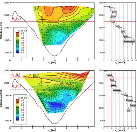
© EGU 2003 Integration from the valley floor h0up to the height ht, where the valley breeze ceases
and vpchanges sign (Fig.3), yields the horizontal mass flux
Fy =
Zht
h0
ρ(z) · vp(z) · B(z)d z, (2)
where B(z) is the valley width at height z. In the cases investigated in this study, the wind direction above the valley breeze layer was always opposite to the valley breeze
5
flow. Hence, vpalways changed sign at the valley breeze top. Even if the flow above the valley breeze is in the same direction as the valley breeze itself, a minimum in the wind velocities between both layers and atmospheric stability changes with height can usually be observed and used to determine ht. The mean uncertainty of an individ-ual horizontal mass flux calculation due to the wind measurement uncertainty can be
10
shown to be ± 7 %. Measurements at two cross sections are not done at the same time. A temporal correction for the horizontal mass flux is applied by using its temporal evolution derived from subsequent flights.
For nighttime drainage flows, different methods to quantify Fy have been used in other studies, showing uncertainties arising from individual vertical profile
measure-15
ments (King, 1989). In contrast, individual vertical profiles used in this study do not represent a vertical profile above a single point at the cross section, but represent an average for the whole cross section. Horizontal mass fluxes were calculated with the individual vertical profile method and from two-dimensional interpolations of the mea-sured wind data at the cross sections. Both methods varied only ± 7 to 11 % from
20
each other, depending on interpolation scheme (Kriging, Inverse-Distance or Linear interpolation) and parameter settings (scaling of vertical to horizontal distance).
The change of the valley breeze layer air mass with time is governed by the change of the valley breeze layer height with time (Fig.3)
FV BL = mV (hl(t2)) − mV (hl(t1))
t2− t1 , (3)
ACPD
3, 5205–5236, 2003 Topographic venting S. Henne et al. Title Page Abstract Introduction Conclusions References Tables Figures J I J I Back CloseFull Screen / Esc
Print Version Interactive Discussion
© EGU 2003 where hl is the mean height of valley breeze layer at the lower and the upper cross
section. The valley’s air mass, mV, is derived from digitized topographic data and for standard atmospheric conditions. The time difference, t2− t1, between two cross-sectional flights was typically about two hours. During the VOTALP campaign valley-parallel wind velocities were continuously measured with scintillometers (Poggio et al.,
5
2000), showing only small variations in the average up-valley flow during daytime. In addition, the wind velocity measured within 10-minute intervals at surface stations in the Leventina valley deviated only by 16 % from the two-hour averages. This underlines the stationary upvalley flow and justifies the assumptions made for the mass budget calculation. In contrast, an observational and numerical study in the nearby Riviera
10
valley shows that the structure and intensity of the valley breeze undergoes significant changes during the day and shows intermittent character (De Wekker et al.,2003). This might be due to different valley configuration and different synoptical forcing. For mass budget calculations like the one presented here the spatial and temporal homogeneity of the valley breeze has to be inspected.
15
2.3. Lidar
The nadir-pointing backscatter lidar, operated by the DLR (Kiemle et al., 1995), was used to observe the structure of the ABL at the wavelength λ = 354, 532 and 1064 nm. The backscatter ratio β, which is determined by the lidar, is the ratio of the total backscatter (Mie+ Rayleigh) to Rayleigh backscatter. Since high relative humidity (RH)
20
values lead to aerosol growth and therefore enhanced Mie scatter, β is enhanced in regions with high aerosol concentration and high RH. Hence, a direct comparison in terms of aerosol concentrations between different altitudes and distant regions is not possible.
ACPD
3, 5205–5236, 2003 Topographic venting S. Henne et al. Title Page Abstract Introduction Conclusions References Tables Figures J I J I Back CloseFull Screen / Esc
Print Version Interactive Discussion
© EGU 2003 2.4. Forward trajectories
To analyze the pathways of pollutants exported to the FT, forward trajectories were ini-tialized at three sites north and south of the main Alpine crest and at different altitudes. We used the FLEXTRA trajectory model (Stohl et al.,1995) based on European Center for Medium-Range Weather Forecasts (ECMWF) analysis.
5
For the years 2000 and 2001, days that were favorable for topographic venting were selected. Since the energy flux at the Earth’s surface plays a very important role in supporting thermal wind systems a simple criterion to select fair weather days was chosen. Days with more than 9 hours of sunshine at selected stations at the northern and the southern side of the main Alpine crest within Switzerland were selected. Ten
10
stations, covering the whole Swiss plateau, and four stations, covering the Ticino area in the south, were chosen. 50 % of the northern stations and 50 % of the southern stations had to fulfill the criterion. A total of 101 days within the two-year period were selected. The selected days lie in the period from the end of March to the beginning of October. Sunshine data was taken from the automatic network of meteorological
15
observations maintained by the Swiss national weather service (MeteoSwiss).
3. Results
3.1. Export of boundary layer air
Horizontal mass fluxes and the change of the valley breeze layer mass with time were computed from a database of 8 flights within both valleys and from digitized
20
topographic information. In order to compare the vertical mass fluxes estimated with the budget method these fluxes are normalized by the length of the investigated valley segment and the air mass of the valley breeze layer, respectively. In this way, the mass export per unit valley length and the fraction of ABL air exported per hour is obtained for each valley. We derived an average net vertical export of 33 % of the valley breeze
ACPD
3, 5205–5236, 2003 Topographic venting S. Henne et al. Title Page Abstract Introduction Conclusions References Tables Figures J I J I Back CloseFull Screen / Esc
Print Version Interactive Discussion
© EGU 2003 layer air mass per hour (Table 1). This export rate is similar in both Mesolcina and
Leventina valleys, and was somewhat higher in June compared to July and August. In June the vertical mass flux per valley length Fz,N is twice as high as in July and August. On the other hand the valley breeze layer height was also larger in June so that the export rate is only one third larger in June compared to July and August.
5
These differences are probably due to weaker atmospheric stability in June.
Valley breeze conditions persist for about 7 - 9 h d−1 during the summer season at this latitude, resulting in venting to the lower FT of 2.3 - 3.0 times the valley breeze layer air mass per day.
10
3.2. Boundary layer structure
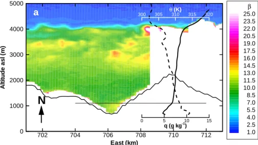
Figures4to6shows a sequence of three cross-valley transects from north (Fig.4) to south (Fig.6) within the Leventina valley. Two different aerosol layers are evident. The area below 1100 m a.s.l. can be interpreted as the convective boundary layer within the valley. Comparison with balloon soundings of potential temperature θ and specific
15
humidity q (Fig.4) shows that the height of the convective boundary layer is even below the altitude of high β. The convective boundary layer is visually indicated by constant to decreasing θ with height and large specific humidity. The convective boundary layer height shown here is relatively low compared to other days. Unfortunately there are no backscatter data available on other days. Typically, a height of 2000 m a.s.l. was
20
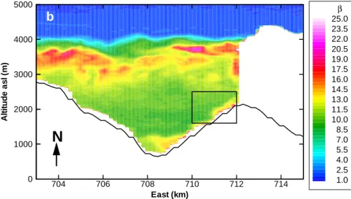
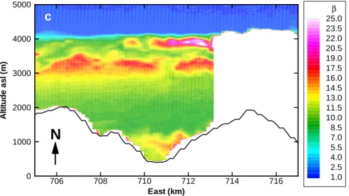
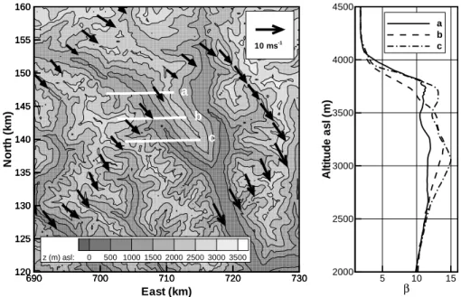
observed from potential temperature profiles. Above 1600 m a.s.l. within the second layer, which reaches up to 4.1 km a.s.l., the prevailing wind was coming from west to northwest. This can be seen in Fig.7, showing wind data measured by the MERLIN IV at an altitude of ∼3900 m a.s.l. Horizontally averaged backscatter ratios increased from northwest to southeast (Fig.7), indicating the additional injection of ABL air into
25
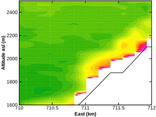
the second layer while being advected horizontally by the synoptic flow. Increased backscatter ratios are also observed in the slope wind layer (Figs.5,8), indicating up-slope transport of aerosols and moisture from the ABL.
ACPD
3, 5205–5236, 2003 Topographic venting S. Henne et al. Title Page Abstract Introduction Conclusions References Tables Figures J I J I Back CloseFull Screen / Esc
Print Version Interactive Discussion
© EGU 2003 Assuming that the whole vertical mass flux, as derived by the budget method,
oc-curs within the slope wind system, the corresponding slope wind depth was evaluated. Typical slope wind velocities measured during the CHAPOP campaign were ∼2 m s−1. The estimated slope wind depth of ∼100 m is similar to depths observed directly in other studies (Kossmann et al., 1999). This suggests that slope winds are the most
5
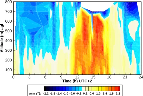
important mechanism for vertical export of ABL air. This is also supported by strong upward motion observed by the sodar wind profiling system (Fig.9) above the crest, where the winds of both slopes merge. Vertical velocities of more than ∼1.5 m s−1can be seen from 10:00 UTC to 16:00 UTC ranging up to 700 m above ground level. During the night sinking motion persists due to the larger scale subsidence and possibly local
10
down-slope flow. However, the downward motion during the night is much weaker than the upward motion during the day.
Ground based lidar observations in the Mesolcina valley during VOTALP showed an increase in backscatter ratios above crest height in the afternoon hours (Carnuth and Trickl,2000). In addition, the increase of VOC concentrations above crest height
be-15
tween morning and afternoon could be related to vertical transport of in-valley traffic emissions (Prevot et al.,2000). In other studies, elevated layers have been observed downwind of the Alps and over the Adriatic Sea (Nyeki et al., 2002), indicating hor-izontal transport of ABL air masses that might have been lifted above mountainous terrain. Even further away above the Mediterranean elevated layers are frequently
ob-20
served (Lelieveld et al.,2002), caused by other lifting processes including topographic venting.
3.3. Forward trajectories
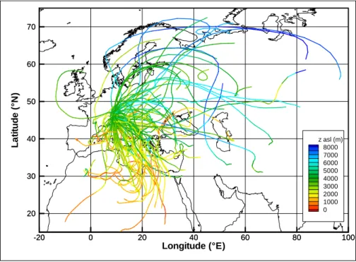
On days with fair weather conditions for the years 2000 and 2001, two ensembles of forward trajectories with an initial altitude of 3500 m a.s.l. were identified (Figs. 10
25
and 11). This altitude corresponds with the altitude that is reached by topographic venting. In the first ensemble, air masses move in a southerly direction and slowly descend within the subtropical anticyclone above the Mediterranean and North Africa.
ACPD
3, 5205–5236, 2003 Topographic venting S. Henne et al. Title Page Abstract Introduction Conclusions References Tables Figures J I J I Back CloseFull Screen / Esc
Print Version Interactive Discussion
© EGU 2003 Contained pollutants possibly influence surface concentrations or remain in reservoir
layers (Lelieveld et al.,2002;Traub et al.,2003). In the second ensemble, air masses move northward and ascend up to 9000 m a.s.l. influencing the whole tropospheric column, experiencing increased westerly flow and leading to transport towards Asia. These results look similar for all three sites where trajectories were initialized.
How-5
ever, the results change for different initial altitudes (Fig. 12). North of the Alps the differences in initial altitudes disappear. South of the Alps lower initial altitudes cause the air to descend faster and travel slower southwards than for higher initial altitudes. Only 1 % of all forward trajectories initialized below 2 km a.s.l. reach the FT south of 20◦ N within 8 days. In contrast, 10 % of trajectories initialized at 3500 m a.s.l. arrive
10
in the same region and within the same time, and begin to ascend in the intertropical convergence zone (ITCZ) potentially reaching the upper troposphere and lower strato-sphere. Obviously, this pathway for European ABL pollutants is a result of preceding topographic venting above the Alps.
4. Discussion
15
Our investigations of the daytime valley atmosphere under fair weather conditions are schematically summarized in Fig.13. Pollutants are emitted mainly at the valley floor or advected horizontally by the valley breeze from the forelands. Within the valley, a well-mixed boundary layer (NOxmixing ratios of about 10 ppbv) is capped by a rather stable layer indicated by an increase of potential temperature (dashed-dotted line). Up-slope
20
winds are able to penetrate this layer and lift polluted air from lower levels. Additional shallow cumulus cloud formation above the crests further maintains vertical motion. Above the stable layer horizontal airflow is mainly synoptically driven. In contrast to the ABL, the upper layer is only partly mixed and is indirectly connected to the surface, therefore the term “injection layer” is used (NOx ∼1 ppbv). The injection layer is capped
25
by a strong inversion that marks the transition to the FT (NOx∼0.1 ppbv). The mass balance of the slope flow system is not closed in the two-dimensional valley cross
sec-ACPD
3, 5205–5236, 2003 Topographic venting S. Henne et al. Title Page Abstract Introduction Conclusions References Tables Figures J I J I Back CloseFull Screen / Esc
Print Version Interactive Discussion
© EGU 2003 tion but in a three dimensional way by the valley breeze.
Extrapolating the high export rates derived for the Leventina and the Mesolcina val-leys to the whole Alpine region, we estimated the total NOx export by thermal wind systems in the Alps. A calculation that considers advection from the forelands, accu-mulation of nighttime emissions in the ABL, but no day-to-day accuaccu-mulation or chemical
5
transformation, yields an estimated total NOxexport of ∼0.2 Gg(N) per day. This corre-sponds to ∼50 % of daily NOxemissions in the region influenced by plain-to-mountain flows (area enclosed by the thin white line in Fig.1). The annual average NOx+ PAN export of the European ABL has been estimated at 21 % of total emissions using a GCTM (Wild and Akimoto, 2001). This suggests that on fair weather days
pollu-10
tant export by thermal wind systems enhances export by a factor of ∼2.5 in the Alps. This enhancement, yet unconsidered in GCTMs, will also occur within other European mountainous regions, such as the Pyrenees and Apennines.
O3 concentrations in the ABL are typically high (> 80 ppbv O3) for the inves-tigated weather conditions and for air masses advected from the Po Basin (
Pre-15
vot et al., 1997). Heavy goods and passenger traffic through the Swiss Alps have increased by 72 % and 18 % in the last decade, respectively, and are expected to grow in the future. Due to enhanced O3 production efficiency in the FT (∼25 (molec. O3) / (molec. NOx) in the spring time FT above the Alps (Carpenter et al., 2000) and ∼5 (molec. O3) / (molec. NOx) in the European ABL (Hov and Flatoy,1997))
20
and rapid vertical transport, a NOxmolecule emitted in an Alpine valley and lifted to the FT produces more O3than a NOxmolecule above flat terrain. Therefore considerable amounts of O3are exported directly and indirectly to the FT.
5. Conclusions
25
Topographic venting of ABL air from deep Alpine valleys to the FT was quantified from observed air mass budgets for two Alpine valleys during three aircraft campaigns. As
ACPD
3, 5205–5236, 2003 Topographic venting S. Henne et al. Title Page Abstract Introduction Conclusions References Tables Figures J I J I Back CloseFull Screen / Esc
Print Version Interactive Discussion
© EGU 2003 much as 3 times the valley breeze layer air mass is exported on a summer time fair
weather day. Observations of atmospheric backscatter ratios observed by an airborne lidar confirm this venting mechanism. Pollutants and moisture are exported from the ABL within the valley to the injection layer. This layer reaches up well above crest height to about 4000 m a.s.l. Our observations also suggest that daytime slope winds are the
5
main mechanism driving vertical export. Pollutants trapped in the injection layer leave the mountainous terrain well above the ABL of the forelands, and therefore become part of the FT. About 50 days with strong solar insolation within the summer months favor topographic venting. Trajectory studies for these days show that the initial height above the Alps determines how fast and at which altitude an air mass is transported
10
southward, exporting European air pollutants which were lifted by topographic venting above the Alps.
Topographic venting is expected to play a more important role in Europe than in North America and Asia where pollutant export is influenced more strongly by warm conveyer belts (upward airflow within extratropical cyclone ahead of the cold front) that
15
are less frequently observed in Europe (Stohl,2001).
Since 27 % of the Earth’s land surface is defined as mountainous (altitude > 1500 m a.s.l.) (Messerli and Ives,1997) and mountain ranges lower than the Alps tend to force thermal convection as well (Kossmann et al.,1999), topographic venting is not only of regional European but of global importance. However, complex topography is only
20
treated on a sub-grid scale in GCTMs, consequently topographic venting is not rep-resented properly (Noppel and Fiedler,2002). Development of a suitable topographic venting parameterization for GCTMs will help to better quantify the effects of thermal air flow in mountainous terrain on continental and global tropospheric pollution budgets.
Investigations on a climatological scale, e.g. long term lidar studies or analysis of
25
operationally available sounding data, could verify the significance of the topographic venting mechanism. The chemical composition of the ABL and the injection layer was analyzed during both VOTALP and CHAPOP campaign. The gathered information will be used to quantify the expected O3production efficiency enhancement in an air mass
ACPD
3, 5205–5236, 2003 Topographic venting S. Henne et al. Title Page Abstract Introduction Conclusions References Tables Figures J I J I Back CloseFull Screen / Esc
Print Version Interactive Discussion
© EGU 2003 lifted to the injection layer.
Acknowledgements. Support by the European Commission for the projects VOTALP and
CAATER is acknowledged. Ground based meteorological data and flight planing support was provided by MeteoSwiss. Special thanks go to V. Fumagalli and the Kanton Ticino for support-ing the build-up of the measurement sites dursupport-ing the CHAPOP campaign. We also like to thank
5
the crews or the DLR Falcon, the Meteo France MERLIN IV, the MetAir and all involved groups in both projects.
References
Atkinson, B. W. and Shahub, A. N.: Orographic and Stability Effects on Daytime, Valley-Side Slope Flows, Boundary-Layer Meteorology, 68, 275–300, 1994. 5210
10
Berkowitz, C. M., Fast, J. D., and Easter, R. C.: Boundary layer vertical exchange processes and the mass budget of ozone: Observations and model results, Journal of Geophysical Research-Atmospheres, 105, 14 789–14 805, 2000. 5207
Carnuth, W. and Trickl, T.: Transport studies with the IFU three-wavelength aerosol lidar during the VOTALP Mesolcina experiment, Atmospheric Environment, 34, 1425–1434, 2000. 5215
15
Carpenter, L. J., Green, T. J., Mills, G. P., Bauguitte, S., Penkett, S. A., Zanis, P., Schuepbach, E., Schmidtbauer, N., Monks, P. S., and Zellweger, C.: Oxidized nitrogen and ozone pro-duction efficiencies in the springtime free troposphere over the Alps, Journal of Geophysical Research, 105, 14 547–14 559, 2000. 5217
Cotton, W., Alexander, G., Hertenstein, R., Walko, R., McAnelly, R., and Nicholls, M.: Cloud
20
venting – A review and some new global annual estimates, Earth-Science Reviews, 39, 169– 206, 1995. 5207
De Wekker, S. F. J., Steyn, D. G., Fast, J. D., Rotach, M. W., and Zhong, S.: The Performance of RAMS in Representing the Convective Boundary Layer Structure in a Very Steep Valley, Environmental Fluid Mechanics, submitted, 2003. 5212
25
Fiedler, F.: Atmospheric Circulation, in Chemistry of the Unpolluted and Polluted Troposphere, edited by Georgii, H. W.and Jaeschke, W., 509, Reidel Publishing Company, Dordrecht, 1982. 5207
ACPD
3, 5205–5236, 2003 Topographic venting S. Henne et al. Title Page Abstract Introduction Conclusions References Tables Figures J I J I Back CloseFull Screen / Esc
Print Version Interactive Discussion
© EGU 2003 Large Valley During Mountain and Valley Wind, Meteorology and Atmospheric Physics, 37,
129–140, 1987. 5210
Furger, M., Dommen, J., Graber, W., Poggio, L., Pr ´ev ˆot, A., Emeis, S., Grell, G., Trickl, T., Gomiscek, B., Neininger, B., and Wotawa, G.: The VOTALP Mesolcina Valley Campaign 1996 – concept, background and some highlights, Atmospheric Environment, 34, 1395–
5
1412, 2000. 5208
Hov, O. and Flatoy, F.: Convective redistribution of ozone and oxides of nitrogen in the tropo-sphere over Europe in summer and fall, Journal of Atmospheric Chemistry, 28, 319–337, 1997. 5217
Jacob, D. J., Prather, M. J., Rasch, P. J., Shia, R. L., Balkanski, Y. J., Beagley, S. R., Bergmann,
10
D. J., Blackshear, W. T., Brown, M., Chiba, M., Chipperfield, M. P., deGrandpre, J., Dignon, J. E., Feichter, J., Genthon, C., Grose, W. L., Kasibhatla, P. S., Kohler, I., Kritz, M. A., Law, K., Penner, J. E., Ramonet, M., Reeves, C. E., Rotman, D. A., Stockwell, D. Z., VanVelthoven, P. F. J., Verver, G., Wild, O., Yang, H., and Zimmermann, P.: Evaluation and intercomparison of global atmospheric transport models using Rn-222 and other short-lived tracers, Journal of
15
Geophysical Research-Atmospheres, 102, 5953–5970, 1997. 5207
Kiemle, C., Kastner, M., and Ehret, G.: The Convective Boundary-Layer Structure from Lidar and Radiosonde Measurements During the Efeda-91 Campaign, Journal of Atmospheric and Oceanic Technology, 12, 771–782, 1995. 5212
King, C. W.: Representativeness of Single Vertical Wind Profiles for Determining Volume Flux
20
in Valleys, Journal of Applied Meteorology, 28, 463–466, 1989. 5211
Kossmann, M., Corsmeier, U., De Wekker, S., Fiedler, F., V ¨ogtlin, R., Kalthoff, N., G¨usten, H., and Neininger, B.: Observations of Handover Processes between the Atmospheric Boundary Layer and the Free Troposphere over Mountainous Terrain, Contributions to Atmospheric Physics, 72, 329–350, 1999. 5207,5215,5218
25
Lelieveld, J. and Crutzen, P. J.: Role of Deep Cloud Convection in the Ozone Budget of the Troposphere, Science, 264, 1759–1761, 1994. 5207
Lelieveld, J., Berresheim, H., Borrmann, S., Crutzen, P. J., Dentener, F. J., Fischer, H., Fe-ichter, J., Flatau, P. J., Heland, J., Holzinger, R., Korrmann, R., Lawrence, M. G., Levin, Z., Markowicz, K. M., Mihalopoulos, N., Minikin, A., Ramanathan, V., de Reus, M., Roelofs, G. J.,
30
Scheeren, H. A., Sciare, J., Schlager, H., Schultz, M., Siegmund, P., Steil, B., Stephanou, E. G., Stier, P., Traub, M., Warneke, C., Williams, J., and Ziereis, H.: Global air pollution crossroads over the Mediterranean, Science, 298, 794–799, 2002. 5215,5216
ACPD
3, 5205–5236, 2003 Topographic venting S. Henne et al. Title Page Abstract Introduction Conclusions References Tables Figures J I J I Back CloseFull Screen / Esc
Print Version Interactive Discussion
© EGU 2003 Lin, X., Trainer, M., and Liu, S. C.: On the Nonlinearity of the Tropospheric Ozone Production,
Journal of Geophysical Research, 93, 15 879–15 888, 1988. 5206
McKendry, I. G. and Lundgren, J.: Tropospheric layering of ozone in regions of urbanized complex and/or coastal terrain: a review, Progress in Physical Geography, 24, 329–354, 2000. 5207
5
Messerli, B. and Ives, J. (Eds.): Mountains of the World: A Global Priority, Parthenon, New York & London, 1997. 5218
Millan, M. M., Sanz, M. J., Salvador, R., and Mantilla, E.: Atmospheric dynamics and ozone cycles related to nitrogen deposition in the western Mediterranean, Environmental Pollution, 118, 167–186, 2002. 5207
10
Neininger, B., Fuchs, W., Baeumle, M., Volz-Thomas, A., Pr ´ev ˆot, A., and Dommen, J.: A small aircraft for more than just ozone: METAIR’s ’DIMONA’ after ten years of evolving develop-ment, in 11th Symposium on Meteorological Observations and Instrumentation, American Meteorological Society, Albuquerque, NM, USA, 2001. 5208
Newell, R. E., Thouret, V., Cho, J. Y. N., Stoller, P., Marenco, A., and Smit, H. G.: Ubiquity of
15
quasi-horizontal layers in the troposphere, Nature, 398, 316–319, 1999. 5207
Noppel, H. and Fiedler, F.: Mesoscale heat transport over complex terrain by slope winds – A conceptual model and numerical simulations, Boundary-Layer Meteorology, 104, 73–97, 2002. 5218
Nyeki, S., Eleftheriadis, K., Baltensperger, U., Colbeck, I., Fiebig, M., Fix, A., Kiemle, C.,
20
Lazaridis, M., and Petzold, A.: Airborne lidar and in-situ aerosol observations of an ele-vated layer, leeward of the European Alps and Apennines, Geophysical Research Letters, 29, 1852, 2002. 5215
Poggio, L. P., Furger, M., Prevot, A. S. H., Graber, W. K., and Andreas, E. L.,: Scintillometer wind measurements over complex terrain, Journal of Atmospheric and Oceanic Technology,
25
17, 17–26, 2000. 5212
Prevot, A. S. H., Staehelin, J., Kok, G. L., Schillawski, R. D., Neininger, B., Staffelbach, T., Nef-tel, A., Wernli, H., and Dommen, J.: The Milan photooxidant plume, Journal of Geophysical Research-Atmospheres, 102, 23 375–23 388, 1997. 5217
Prevot, A. S. H., Dommen, J., and Baeumle, M.: Influence of road traffic on volatile organic
30
compound concentrations in and above a deep Alpine valley, Atmospheric Environment, 34, 4719–4726, 2000. 5215
ACPD
3, 5205–5236, 2003 Topographic venting S. Henne et al. Title Page Abstract Introduction Conclusions References Tables Figures J I J I Back CloseFull Screen / Esc
Print Version Interactive Discussion
© EGU 2003 5206
Stohl, A.: A 1-year Lagrangian “climatology” of airstreams in the Northern Hemisphere tropo-sphere and lowermost stratotropo-sphere, Journal of Geophysical Research-Atmotropo-spheres, 106, 7263–7279, 2001. 5218
Stohl, A., Wotawa, G., Seibert, P., and Kromp-Kolb, H.: Interpolation Errors in Wind Fields
5
as a Function of Spatial and Temporal Resolution and Their Impact on Different Types of Kinematic Trajectories, Journal of Applied Meteorology, 34, 2149–2165, 1995. 5213 Traub, M., Fischer, H., de Reus, M., Korrmann, R., Heland, J., Ziereis, H., Schlager, H.,
Holzinger, R., Warneke, C., de Gouw, J. A., and Lelieveld, J.: Chemical characteristics assigned to trajectory clusters during the MINOS campaign, Atmospheric Chemistry and
10
Physics Discussions, 3, 107–134, 2003. 5216
Tyson, P. D. and D’Abreton, P. C.: Transport and recirculation of aerosols off southern Africa -Macroscale plume structure, Atmospheric Environment, 32, 1511–1524, 1998. 5207 Vergeiner, I. and Dreiseitl, E.: Valley Winds and Slope Winds – Observations and Elementary
Thoughts, Meteorology and Atmospheric Physics, 36, 264–286, 1987. 5210
15
Whiteman, C. D.: Mountain Meteorology, Oxford University Press, New York, 2000. 5209 Wild, O. and Akimoto, H.: Intercontinental transport of ozone and its precursors in a
three-dimensional global CTM, Journal of Geophysical Research-Atmospheres, 106, 27 729– 27 744, 2001. 5217
Wotawa, G. and Kromp-Kolb, H.: The research project VOTALP – general objectives and main
20
ACPD
3, 5205–5236, 2003 Topographic venting S. Henne et al. Title Page Abstract Introduction Conclusions References Tables Figures J I J I Back CloseFull Screen / Esc
Print Version Interactive Discussion
© EGU 2003
Table 1. Net vertical mass export of the investigated valleys. Mean standard deviation of
individual flux measurements is given in parentheses and derived from standard deviation of the up-valley wind velocity at each altitude level used for the horizontal flux calculation
Number −Fy,i n −Fy ,out FV BL Fz F a z,N Export rate b Valley of flights (T gh) (T gh) (T gh ) (T gh) (h kmT g ) (%h) Leventina (August ’01) 4 51 (3) 22 (3) 5.6 24 (4) 1.5 (0.3) 30 (5) Mesolcina (July ’96) 2 69 (5) 35 (1) -1.4 35 (5) 1.8 (0.3) 28 (4) Mesolcina (June ’98) 2 113 (5) 38 (3) 3.2 71 (5) 3.7 (0.4) 42 (3) Average - - - - 39 2.1 33 a
The net vertical mass flux divided by the length of the valley segment.
b
ACPD
3, 5205–5236, 2003 Topographic venting S. Henne et al. Title Page Abstract Introduction Conclusions References Tables Figures J I J I Back CloseFull Screen / Esc
Print Version Interactive Discussion
© EGU 2003
Fig. 1. Investigated valleys in southern Switzerland. White solid lines a-c indicate lidar transects above the Leventina Valley. Black solid lines represent cross-sectional flights of the MetAir aircraft used for the mass budget calculation.
20
Fig. 1. Investigated valleys in southern Switzerland. White solid lines a–c indicate lidar
tran-sects above the Leventina Valley. Black solid lines represent cross-sectional flights of the MetAir aircraft used for the mass budget calculation.
ACPD
3, 5205–5236, 2003 Topographic venting S. Henne et al. Title Page Abstract Introduction Conclusions References Tables Figures J I J I Back CloseFull Screen / Esc
Print Version Interactive Discussion
© EGU 2003
Fig. 2. Air flow in the Leventina valley at 10 UTC on 26 August 2001. Horizontal mass fluxes
Fy,inandFy,outand change of valley breeze layer air mass with timeFV BLas measured by the MetAir aircraft. The horizontal direction xn is perpendicular to the valley axis, the y direction points down-valley. The contour plot depicts wind velocity parallel to the valley axisvp. Negative values indicate up-valley flow, positive values down-valley flow.
21
Fig. 2. Air flow in the Leventina valley at 10:00 UTC on 26 August 2001. Horizontal mass fluxes
Fy,i n and Fy,out and change of valley breeze layer air mass with time FV BLas measured by the
MetAir aircraft. The horizontal direction xn is perpendicular to the valley axis, the y direction
points down-valley. The contour plot depicts wind velocity parallel to the valley axis vp. Negative
values indicate up-valley flow, positive values down-valley flow. 5225
ACPD
3, 5205–5236, 2003 Topographic venting S. Henne et al. Title Page Abstract Introduction Conclusions References Tables Figures J I J I Back CloseFull Screen / Esc
Print Version Interactive Discussion © EGU 2003 xn(km) A lt it u d e a s l (m ) 0 1 2 3 4 5 6 7 500 1000 1500 2000 2500 xn(km) A lt it u d e a s l (m ) 0 1 2 3 4 5 6 7 500 1000 1500 2000 2500 0 1 2 3 4 5 6 7 500 1000 1500 2000 2500 v p(m s -1) 2.0 1.0 0.0 -1.0 -2.0 -3.0 -4.0 -5.0 -6.0 ht,1(t1) 0 1 2 3 4 5 6 7 500 1000 1500 2000 2500 v p(m s -1) 2.0 1.0 0.0 -1.0 -2.0 -3.0 -4.0 -5.0 -6.0 ht,1(t1) ht,1(t2) vp(m s -1-3) -4 -5 -6 -2 -1 0 1 2 500 1000 1500 2000 2500 vp(m s -1 ) -6 -5 -4 -3 -2 -1 0 1 2 500 1000 1500 2000 2500
Fig. 3. Change of valley breeze with time. Contour plot (left) of valley parallel wind velocityvpat
cross-section within Leventina valley on 28 August 11:45 UTC (upper figures) and 13:30 UTC (lower figures) and vertical profile of horizontal averaged vp (right). Change of valley breeze
layer height zV BL with time is indicated in lower figure. The example shows a rather strong
change of the valley breeze layer height to illustrate the effect. Usually the change of the valley breeze layer height was much smaller.
22
Fig. 3. Change of valley breeze with time. Contour plot (left) of valley parallel wind velocity vpat
cross-section within Leventina valley on 28 August 11:45 UTC (upper figures) and 13:30 UTC (lower figures) and vertical profile of horizontal averaged vp(right). Change of valley breeze
layer height zV BL with time is indicated in lower figure. The example shows a rather strong
change of the valley breeze layer height to illustrate the effect. Usually the change of the valley breeze layer height was much smaller.
ACPD
3, 5205–5236, 2003 Topographic venting S. Henne et al. Title Page Abstract Introduction Conclusions References Tables Figures J I J I Back CloseFull Screen / Esc
Print Version Interactive Discussion © EGU 2003 East (km) A lt it u d e a s l (m ) 702 704 706 708 710 712 0 1000 2000 3000 4000 5000 β 25.0 23.5 22.0 20.5 19.0 17.5 16.0 14.5 13.0 11.5 10.0 8.5 7.0 5.5 4.0 2.5 1.0
a
N
θ(K) q (g kg-1) 300 305 310 315 320 0 5 10 15Fig. 4. Atmospheric backscatter ratio
β
for lidar transect within the Leventina valley on 28
August 2001 from 13:36 and 13:56 UTC,
λ
= 1064 nm. Horizontal coordinates refer to Swiss
coordinate system. Transect corresponds to white solid lines labeled a in Fig. 1 and Fig. 7. The
surface as seen by the lidar differs slightly from digitized topographic data with 250 m x 250 m
horizontal resolution (black solid line). The lidar beam does not penetrate clouds, represented
by white areas. Potential temperature
θ
(solid black line) and specific humidity q (dashed black
line) as measured by a radio sonde launched at 12 UTC at the valley floor close to the transect
are included.
23
Fig. 4. Atmospheric backscatter ratio β for lidar transect within the Leventina valley on 28
August 2001 from 13:36 and 13:56 UTC, λ= 1064 nm. Horizontal coordinates refer to Swiss coordinate system. Transect corresponds to white solid lines labeled a in Fig. 1 and Fig. 7. The surface as seen by the lidar differs slightly from digitized topographic data with 250 m × 250 m horizontal resolution (black solid line). The lidar beam does not penetrate clouds, represented by white areas. Potential temperature θ (solid black line) and specific humidity q (dashed black line) as measured by a radio sonde launched at 12:00 UTC at the valley floor close to the transect are included.
ACPD
3, 5205–5236, 2003 Topographic venting S. Henne et al. Title Page Abstract Introduction Conclusions References Tables Figures J I J I Back CloseFull Screen / Esc
Print Version Interactive Discussion © EGU 2003 East (km) A lt it u d e a s l (m ) 704 706 708 710 712 714 0 1000 2000 3000 4000 5000 β 25.0 23.5 22.0 20.5 19.0 17.5 16.0 14.5 13.0 11.5 10.0 8.5 7.0 5.5 4.0 2.5 1.0
b
N
Fig. 5. Same as Fig. 4 but for transect b. See Fig. 8 for blow up of slope wind layer (black
rectangle).
East (km) A lt it u d e a s l (m ) 706 708 710 712 714 716 0 1000 2000 3000 4000 5000 β 25.0 23.5 22.0 20.5 19.0 17.5 16.0 14.5 13.0 11.5 10.0 8.5 7.0 5.5 4.0 2.5 1.0c
N
Fig. 6. Same as Fig. 4 but for transect c.
24
Fig. 5. Same as Fig. 4 but for transect b. See Fig.8 for blow up of slope wind layer (black rectangle).
ACPD
3, 5205–5236, 2003 Topographic venting S. Henne et al. Title Page Abstract Introduction Conclusions References Tables Figures J I J I Back CloseFull Screen / Esc
Print Version Interactive Discussion © EGU 2003 East (km) A lt it u d e a s l (m ) 704 706 708 710 712 714 0 1000 2000 3000 4000 5000 β 25.0 23.5 22.0 20.5 19.0 17.5 16.0 14.5 13.0 11.5 10.0 8.5 7.0 5.5 4.0 2.5 1.0
b
N
Fig. 5. Same as Fig. 4 but for transect b. See Fig. 8 for blow up of slope wind layer (black
rectangle).
East (km) A lt it u d e a s l (m ) 706 708 710 712 714 716 0 1000 2000 3000 4000 5000 β 25.0 23.5 22.0 20.5 19.0 17.5 16.0 14.5 13.0 11.5 10.0 8.5 7.0 5.5 4.0 2.5 1.0c
N
Fig. 6. Same as Fig. 4 but for transect c.
24
ACPD
3, 5205–5236, 2003 Topographic venting S. Henne et al. Title Page Abstract Introduction Conclusions References Tables Figures J I J I Back CloseFull Screen / Esc
Print Version Interactive Discussion © EGU 2003 690 700 710 720 730 120 125 130 135 140 145 150 155 160 z (m) asl: 0 500 1000 1500 2000 2500 3000 3500 690 700 710 720 730 120 125 130 135 140 145 150 155 160 East (km) N o rt h (k m ) 690 700 710 720 730 120 125 130 135 140 145 150 155 160 10 ms-1 a b c β A lt it u d e a s l (m ) 5 10 15 2000 2500 3000 3500 4000 4500 a b c
Fig. 7. Left: Flow at 3900 m asl above Leventina valley, 28 August 2001, 12 UTC. Coordinates refer to Swiss coordinate system. White solid lines represent lidar transects in Fig. 4 to 6. The length of the vectors are proportional to the wind velocity. Right: Mean vertical profiles of backscatter ratioβfor transects a-c.
25
Fig. 7. Left: Flow at 3900 m a.s.l. above Leventina valley, 28 August 2001, 12:00 UTC.
Coordinates refer to Swiss coordinate system. White solid lines represent lidar transects in Figs.4to6. The length of the vectors are proportional to the wind velocity. Right: Mean vertical profiles of backscatter ratio β for transects a–c.
ACPD
3, 5205–5236, 2003 Topographic venting S. Henne et al. Title Page Abstract Introduction Conclusions References Tables Figures J I J I Back CloseFull Screen / Esc
Print Version Interactive Discussion © EGU 2003 East (km) A lt it u d e a s l (m ) 710 710.5 711 711.5 712 1600 1800 2000 2200 2400
Fig. 8. Same as Fig. 5, but
mag-nified slope wind layer.
Time (h) UTC+2 A lt it u d e (m ) a g l 0 3 6 9 12 15 18 21 24 100 200 300 400 500 600 700 800 w(m s-1 ): -2.2 -1.8 -1.4 -1.0 -0.6 -0.2 0.2 0.6 1.0 1.4 1.8 2.2
Fig. 9.
Evolution of vertical
wind velocities above the
north-eastern crest of the Leventina
valley on 28 August 2001.
Yel-low to red colors indicate upward
motion, blue to black colors
indi-cate downward motion.
26
Fig. 8. Same as Fig.5, but magnified slope wind layer.
ACPD
3, 5205–5236, 2003 Topographic venting S. Henne et al. Title Page Abstract Introduction Conclusions References Tables Figures J I J I Back CloseFull Screen / Esc
Print Version Interactive Discussion © EGU 2003 East (km) A lt it u d e a s l (m ) 710 710.5 711 711.5 712 1600 1800 2000 2200 2400
Fig. 8. Same as Fig. 5, but
mag-nified slope wind layer.
Time (h) UTC+2 A lt it u d e (m ) a g l 0 3 6 9 12 15 18 21 24 100 200 300 400 500 600 700 800 w(m s-1 ): -2.2 -1.8 -1.4 -1.0 -0.6 -0.2 0.2 0.6 1.0 1.4 1.8 2.2
Fig. 9.
Evolution of vertical
wind velocities above the
north-eastern crest of the Leventina
valley on 28 August 2001.
Yel-low to red colors indicate upward
motion, blue to black colors
indi-cate downward motion.
26
Fig. 9. Evolution of vertical wind velocities above the north-eastern crest of the Leventina valley
on 28 August 2001. Yellow to red colors indicate upward motion, blue to black colors indicate downward motion.
ACPD
3, 5205–5236, 2003 Topographic venting S. Henne et al. Title Page Abstract Introduction Conclusions References Tables Figures J I J I Back CloseFull Screen / Esc
Print Version Interactive Discussion © EGU 2003 -20 0 20 40 60 80 100 20 30 40 50 60 70 Longitude (°E) L a ti tu d e (° N ) -20 0 20 40 60 80 100 20 30 40 50 60 70 z asl (m) 8000 7000 6000 5000 4000 3000 2000 1000 0
Fig. 10. Forward trajectories
ini-tialized at 3428 m asl above
Got-thard region (8
◦58’ E, 46
◦21’ N)
at 16 UTC on fair weather days
for the years 2000 and 2001.
Colors indicate the altitude of
the air mass above sea level.
0 10 20 30 40 50 60 70 80 0 1000 2000 3000 4000 5000 6000 7000 8000 9000 10000 Hours: 0 24 48 72 96 120 144 168 Latitude [deg] A lt it u d e (m ) a s l 0 10 20 30 40 50 60 70 80 0 1000 2000 3000 4000 5000 6000 7000 8000 9000 10000
Fig. 11. Altitude of the
trajec-tories shown in Fig. 10 versus
latitude. Symbols represent
in-dividual trajectory points. Color
coding refers to the hours since
the trajectory was started. The
black line indicates the median
height of all trajectory points in
5
◦latitudinal bins.
Thin black
lines represent the
correspond-ing lower and upper quartiles.
27
Fig. 10. Forward trajectories initialized at 3428 m a.s.l. above Gotthard region (8◦ 58’ E, 46◦ 21’ N) at 16:00 UTC on fair weather days for the years 2000 and 2001. Colors indicate the altitude of the air mass above sea level.
ACPD
3, 5205–5236, 2003 Topographic venting S. Henne et al. Title Page Abstract Introduction Conclusions References Tables Figures J I J I Back CloseFull Screen / Esc
Print Version Interactive Discussion © EGU 2003 -20 0 20 40 60 80 100 20 30 40 50 60 70 Longitude (°E) L a ti tu d e (° N ) -20 0 20 40 60 80 100 20 30 40 50 60 70 z asl (m) 8000 7000 6000 5000 4000 3000 2000 1000 0
Fig. 10. Forward trajectories
ini-tialized at 3428 m asl above
Got-thard region (8
◦58’ E, 46
◦21’ N)
at 16 UTC on fair weather days
for the years 2000 and 2001.
Colors indicate the altitude of
the air mass above sea level.
0 10 20 30 40 50 60 70 80 0 1000 2000 3000 4000 5000 6000 7000 8000 9000 10000 Hours: 0 24 48 72 96 120 144 168 Latitude [deg] A lt it u d e (m ) a s l 0 10 20 30 40 50 60 70 80 0 1000 2000 3000 4000 5000 6000 7000 8000 9000 10000
Fig. 11. Altitude of the
trajec-tories shown in Fig. 10 versus
latitude. Symbols represent
in-dividual trajectory points. Color
coding refers to the hours since
the trajectory was started. The
black line indicates the median
height of all trajectory points in
5
◦latitudinal bins.
Thin black
lines represent the
correspond-ing lower and upper quartiles.
27
Fig. 11. Altitude of the trajectories shown in Fig. 10versus latitude. Symbols represent indi-vidual trajectory points. Color coding refers to the hours since the trajectory was started. The black line indicates the median height of all trajectory points in 5◦ latitudinal bins. Thin black lines represent the corresponding lower and upper quartiles.
ACPD
3, 5205–5236, 2003 Topographic venting S. Henne et al. Title Page Abstract Introduction Conclusions References Tables Figures J I J I Back CloseFull Screen / Esc
Print Version Interactive Discussion © EGU 2003 Latitude (°N) A lt it u d e (m ) a s l 0 10 20 30 40 50 60 70 80 0 1000 2000 3000 4000 5000 6000 7000 8000 9000 10000
Start Height 1328 (m) asl Start Height 2528 (m) asl Start Height 3428 (m) asl Start Height 4028 (m) asl
Fig. 12.
Median altitude of
trajectories versus latitude (
5
◦bins). Ensembles with different
initial altitudes.
Fig. 13.
Schematic of the
daytime atmospheric structure
and vertical pollution transport
in and above deep Alpine
val-leys.
Altitudes given
repre-sent typical values for the cases
studied.
Typical potential
tem-perature profile is indicated by
dashed red line. See text for
de-tails.
28
Fig. 12. Median altitude of trajectories versus latitude (5◦ bins). Ensembles with different initial
altitudes.
ACPD
3, 5205–5236, 2003 Topographic venting S. Henne et al. Title Page Abstract Introduction Conclusions References Tables Figures J I J I Back CloseFull Screen / Esc
Print Version Interactive Discussion © EGU 2003 Latitude (°N) A lt it u d e (m ) a s l 0 10 20 30 40 50 60 70 80 0 1000 2000 3000 4000 5000 6000 7000 8000 9000 10000
Start Height 1328 (m) asl Start Height 2528 (m) asl Start Height 3428 (m) asl Start Height 4028 (m) asl
Fig. 12.
Median altitude of
trajectories versus latitude (
5
◦bins). Ensembles with different
initial altitudes.
Fig. 13.
Schematic of the
daytime atmospheric structure
and vertical pollution transport
in and above deep Alpine
val-leys.
Altitudes given
repre-sent typical values for the cases
studied.
Typical potential
tem-perature profile is indicated by
dashed red line. See text for
de-tails.
28
Fig. 13. Schematic of the daytime atmospheric structure and vertical pollution transport in
and above deep Alpine valleys. Altitudes given represent typical values for the cases studied. Typical potential temperature profile is indicated by dashed red line. See text for details.

![[PDF] Cours de programmation web coté serveur | Cours Informatique](data:image/gif;base64,R0lGODlhAQABAIAAAP///wAAACH5BAEAAAAALAAAAAABAAEAAAICRAEAOw==)