HAL Id: hal-00295394
https://hal.archives-ouvertes.fr/hal-00295394
Submitted on 9 Feb 2004
HAL is a multi-disciplinary open access
archive for the deposit and dissemination of
sci-entific research documents, whether they are
pub-lished or not. The documents may come from
teaching and research institutions in France or
abroad, or from public or private research centers.
L’archive ouverte pluridisciplinaire HAL, est
destinée au dépôt et à la diffusion de documents
scientifiques de niveau recherche, publiés ou non,
émanant des établissements d’enseignement et de
recherche français ou étrangers, des laboratoires
publics ou privés.
(MAX-DOAS)
G. Hönninger, C. von Friedeburg, U. Platt
To cite this version:
G. Hönninger, C. von Friedeburg, U. Platt. Multi axis differential optical absorption spectroscopy
(MAX-DOAS). Atmospheric Chemistry and Physics, European Geosciences Union, 2004, 4 (1),
pp.231-254. �hal-00295394�
www.atmos-chem-phys.org/acp/4/231/
SRef-ID: 1680-7324/acp/2004-4-231
Chemistry
and Physics
Multi axis differential optical absorption spectroscopy
(MAX-DOAS)
G. H¨onninger1,*, C. von Friedeburg1, and U. Platt1
1Institut f¨ur Umweltphysik, Universit¨at Heidelberg, Heidelberg, Germany *now at: Meteorological Service of Canada, Toronto, Canada
Received: 10 October 2003 – Published in Atmos. Chem. Phys. Discuss.: 11 November 2003 Revised: 31 January 2004 – Accepted: 31 January 2004 – Published: 9 February 2004
Abstract. Multi Axis Differential Optical Absorption
Spec-troscopy (MAX-DOAS) in the atmosphere is a novel mea-surement technique that represents a significant advance on the well-established zenith scattered sunlight DOAS instru-ments which are mainly sensitive to stratospheric absorbers. MAX-DOAS utilizes scattered sunlight received from mul-tiple viewing directions. The spatial distribution of various trace gases close to the instrument can be derived by combin-ing several viewcombin-ing directions. Ground based MAX-DOAS is highly sensitive to absorbers in the lowest few kilome-tres of the atmosphere and vertical profile information can be retrieved by combining the measurements with Radia-tive Transfer Model (RTM) calculations. The potential of the technique for a wide variety of studies of tropospheric trace species and its (few) limitations are discussed. A Monte Carlo RTM is applied to calculate Airmass Factors (AMF) for the various viewing geometries of MAX-DOAS. Airmass Factors can be used to quantify the light path length within the absorber layers. The airmass factor dependencies on the viewing direction and the influence of several parameters (trace gas profile, ground albedo, aerosol profile and type, solar zenith and azimuth angles) are investigated. In addition we give a brief description of the instrumental MAX-DOAS systems realised and deployed so far. The results of the RTM studies are compared to several examples of recent MAX-DOAS field experiments and an outlook for future possible applications is given.
1 Introduction
The analysis of the atmospheric composition by scattered sunlight absorption spectroscopy in the visible/near ultravi-olet spectral ranges has a long tradition. This application is also called “passive” absorption spectroscopy in contrast to
Correspondence to: G. H¨onninger
spectroscopy using artificial light sources (i.e. active DOAS, Perner et al., 1976; Platt et al., 1979; Perner and Platt, 1979; Platt and Perner, 1980; Platt et al., 1980).
Shortly after Dobson and Harrison (1926) conducted mea-surements of atmospheric ozone by passive absorption spec-troscopy, the “Umkehr” technique (G¨otz et al., 1934), which was based on the observation of a few (typically 4) wave-lengths, allowed the retrieval of ozone concentrations in sev-eral atmospheric layers yielding the first vertical profiles of ozone.
The COSPEC (COrrelation SPECtrometer) technique de-veloped in the late 1960s was the first attempt to study tro-pospheric species by analysing scattered sunlight in a wider spectral range while making use of the detailed structure of the absorption bands with the help of an opto-mechanical correlator (Millan et al., 1969; Davies, 1970). It has now been applied for over more than three decades for mea-surements of total emissions of SO2 and NO2 from
var-ious sources, e.g. industrial emissions (Hoff and Millan, 1981) and – in particular – volcanic plumes (e.g. Stoiber and Jepsen, 1973; Hoff et al., 1992).
Scattered sunlight was later used in numerous studies of stratospheric and (in some cases) tropospheric NO2as well
as other stratospheric species by ground-based differential optical absorption spectroscopy (DOAS), as summarised in Table 1. This was a significant step forward, since the quasi-continuous wavelength sampling of DOAS instruments in typically hundreds of spectral channels allows the detection of much weaker absorption features and thus higher sensi-tivity. This is due to the fact that the differential absorption pattern of the trace gas cross section is unique for each ab-sorber and its amplitude can be readily determined by a fit-ting procedure using for example least squares methods to separate the contributions of the individual absorbers. The simultaneous measurement of several absorbers is possible while cross-interferences and the influence of Mie scattering are virtually eliminated.
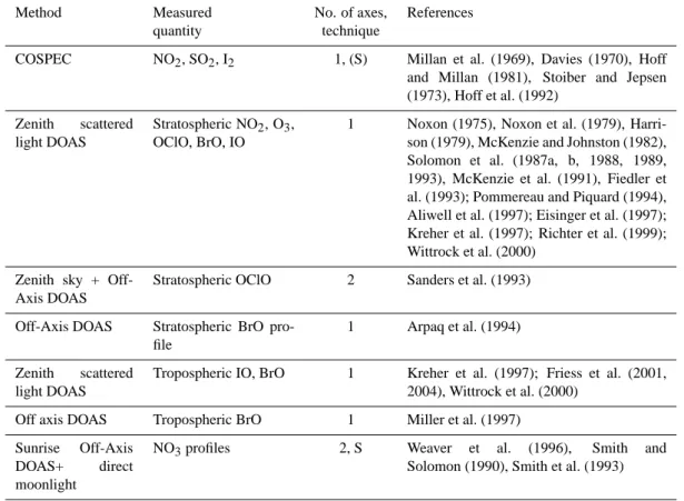
Table 1. Overview and history of the different scattered light passive DOAS applications, # Axis indicates the number of different viewing directions combined.
Method Measured No. of axes, References quantity technique
COSPEC NO2, SO2, I2 1, (S) Millan et al. (1969), Davies (1970), Hoff
and Millan (1981), Stoiber and Jepsen (1973), Hoff et al. (1992)
Zenith scattered light DOAS
Stratospheric NO2, O3,
OClO, BrO, IO
1 Noxon (1975), Noxon et al. (1979), Harri-son (1979), McKenzie and Johnston (1982), Solomon et al. (1987a, b, 1988, 1989, 1993), McKenzie et al. (1991), Fiedler et al. (1993); Pommereau and Piquard (1994), Aliwell et al. (1997); Eisinger et al. (1997); Kreher et al. (1997); Richter et al. (1999); Wittrock et al. (2000)
Zenith sky + Off-Axis DOAS
Stratospheric OClO 2 Sanders et al. (1993)
Off-Axis DOAS Stratospheric BrO pro-file
1 Arpaq et al. (1994)
Zenith scattered light DOAS
Tropospheric IO, BrO 1 Kreher et al. (1997); Friess et al. (2001, 2004), Wittrock et al. (2000)
Off axis DOAS Tropospheric BrO 1 Miller et al. (1997) Sunrise Off-Axis
DOAS+ direct moonlight
NO3profiles 2, S Weaver et al. (1996), Smith and
Solomon (1990), Smith et al. (1993)
Scattered sunlight DOAS measurements yield “slant” col-umn densities of the respective absorbers. Most observations were done with zenith looking instruments because the ra-diative transfer modelling necessary for the determination of vertical column densities is best understood for zenith scat-tered sunlight. On the other hand, for studies of trace species near the ground, artificial light sources (usually high pressure Xenon short arc lamps) were used in active Long-path DOAS experiments (e.g. Perner et al., 1976; Perner and Platt, 1979; Platt et al., 1979; Mount, 1992; Plane and Smith, 1995; Ax-elson et al., 1990; Harder et al., 1997; Stutz and Platt, 1997). These active DOAS measurements yield trace gas concen-trations averaged along the several kilometre long light path, extending from a searchlight type light source to the spec-trometer. Active DOAS instruments have the advantage of allowing measurements to be made independent of daylight and at wavelengths below 300 nm, however, they require a much more sophisticated optical system, more maintenance, and one to two orders of magnitude more power than passive instruments (e.g. Platt, 1994). Therefore a type of instru-ment allowing measureinstru-ments of trace gases near the ground like active DOAS, while retaining the simplicity and self-sufficiency of a passive DOAS instrument, is highly desir-able.
Passive DOAS observations, essentially all using light scattered in the zenith, had already been performed for many years (see Table 1) when the “Off-Axis” geometry (i.e. ob-servation at directions other than towards the zenith) for measurements of scattered sunlight was first introduced by Sanders et al. (1993) to observe OClO over Antarctica dur-ing twilight. The strategy of their study was to observe OClO in the stratosphere using scattered sunlight as long into the “polar night” as possible. As the sun rises or sets, the sky is of course substantially brighter towards the horizon in the direction of the sun compared to the zenith. Thus the light intensity and therefore the signal to noise ratio is improved significantly. Sanders et al. (1993) also pointed out that the off-axis geometry increases the sensitivity for lower absorp-tion layers. They concluded that absorpabsorp-tion by tropospheric species (e.g. O4) is greatly enhanced in the off-axis
view-ing mode, whereas for an absorber in the stratosphere (e.g. NO2) the absorptions for zenith and off-axis geometries are
comparable. Arpaq et al. (1994) used their off-axis obser-vations during morning and evening twilight to derive in-formation on stratospheric BrO at mid-latitudes, including some altitude information from the change in the observed columns during twilight. At the time of the measurements of Arpaq et al. (1994) the available radiative transfer models
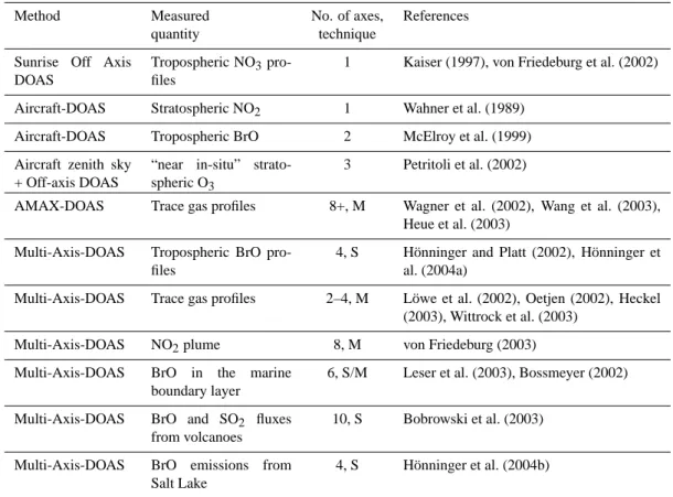
Table 1. Continued.
Method Measured No. of axes, References quantity technique
Sunrise Off Axis DOAS
Tropospheric NO3
pro-files
1 Kaiser (1997), von Friedeburg et al. (2002)
Aircraft-DOAS Stratospheric NO2 1 Wahner et al. (1989)
Aircraft-DOAS Tropospheric BrO 2 McElroy et al. (1999) Aircraft zenith sky
+ Off-axis DOAS
“near in-situ” strato-spheric O3
3 Petritoli et al. (2002)
AMAX-DOAS Trace gas profiles 8+, M Wagner et al. (2002), Wang et al. (2003), Heue et al. (2003)
Multi-Axis-DOAS Tropospheric BrO pro-files
4, S H¨onninger and Platt (2002), H¨onninger et al. (2004a)
Multi-Axis-DOAS Trace gas profiles 2–4, M L¨owe et al. (2002), Oetjen (2002), Heckel (2003), Wittrock et al. (2003)
Multi-Axis-DOAS NO2plume 8, M von Friedeburg (2003)
Multi-Axis-DOAS BrO in the marine boundary layer
6, S/M Leser et al. (2003), Bossmeyer (2002)
Multi-Axis-DOAS BrO and SO2 fluxes
from volcanoes
10, S Bobrowski et al. (2003)
Multi-Axis-DOAS BrO emissions from Salt Lake
4, S H¨onninger et al. (2004b)
S=Scan, M=Multiple telescopes
were single scattering approximations for the off-axis view-ing mode, which was sufficient for the study of stratospheric absorbers.
In spring 1995 Miller et al. (1997) conducted off-axis mea-surements at Kangerlussuaq, Greenland in order to study tro-pospheric BrO and OClO related to boundary layer ozone de-pletion after polar sunrise. These authors observed at off-axis angles (i.e. angle between zenith and observation direction) of 87◦and 85◦, respectively, to obtain a larger signal due to the absorption by the tropospheric BrO fraction. No compar-ison was reported between off-axis and zenith sky measure-ments. The twilight behaviour of the slant columns was used to identify episodes of tropospheric BrO.
Off-axis DOAS, partly in combination with using the moon as direct light source, was also employed for the mea-surement of stratospheric and tropospheric profiles of NO3
by ground based instruments (Weaver et al., 1996; Smith and Solomon, 1990; Smith et al., 1993; Kaiser, 1997; von Friede-burg et al., 2002).
An overview of the different DOAS measurement config-urations and the respective measured quantities reported to date is given in Table 1.
Here we present a new approach to the problem of mea-suring tropospheric species by observing their absorption in
scattered sunlight. This technique combines the advantages of all preceding attempts and introduces several new con-cepts: Combination of measurements at several viewing an-gles, multiple scattering radiative transport modelling, and the use of the O4 absorption to quantify Mie scattering and
aerosols. It allows the study of atmospheric trace gases close to the instrument (i.e. in the boundary layer with ground based instruments) with extreme sensitivity and some de-gree of spatial resolution. While the approaches developed in inversion theory (e.g. Rodgers, 1976) can – and will in the future – be applied to MAX-DOAS, no mathematical inversion was attempted in this study. Profile information was rather derived from the comparison of measurements and various forward modelled profiles. MAX-DOAS instru-ments are very simple in their set-up and can be used from the ground as well as from various airborne platforms.
2 The DOAS technique
Differential Optical Absorption Spectroscopy (DOAS) is a technique that identifies and quantifies trace gas abundances with narrow band absorption structures in the near UV and visible wavelength region in the open atmosphere (e.g. Platt,
1994). The fundamental set-up of a DOAS system consists of a broadband light source, an optical set-up that transfers the light through the atmosphere, and a telescope – spectro-graph – detector system to record the absorption spectra. The basic idea of DOAS is to separate the trace gas absorption cross section into two parts, one that varies “slowly” with wavelength, and a rapidly varying differential cross section
σ0. The latter can be thought of as absorption lines or bands. Broadband extinction by Mie scattering, instrumental effects and turbulence are difficult to quantify, therefore these in-terferences have to be corrected to derive trace gas concen-trations. If the same filtering procedure is applied to the at-mospheric absorption spectrum, the narrow band absorption can be used to calculate the trace gas concentrations (Platt, 1994). The advantages of DOAS are the ability to detect ex-tremely weak absorptions (O.D.∼10−4), the unequivocal and
absolute identification of the trace gases, as well as the fact that trace gas concentrations are determined solely from the absorption cross section. A calibration is therefore not neces-sary. DOAS uses the Beer-Lambert law with modified source intensity I00and absorption cross section σ0to eliminate con-tributions that vary only “slowly” with wavelength:
I (λ) = I00(λ) · e−σ0(λ)·S
S :Slant Column Density (SCD). (1) There are several aspects which are characteristic of scattered sunlight measured by passive DOAS instruments:
2.1 The Fraunhofer reference spectrum
The solar radiation can be described, in first approximation, as the continuous emission of a black body with T ≈5800 K. This continuum, however, is overlaid by a large number of strong absorption lines called the Fraunhofer lines. These lines are due to selective absorption and re-emission of radi-ation by atoms in the solar photosphere. Many solar Fraun-hofer lines are dominant in scattered sunlight DOAS, espe-cially in the UV and visible spectral range (300–600 nm) and are substantially stronger than absorption due to most con-stituents of the terrestrial atmosphere.
Fraunhofer lines have to be carefully removed in the DOAS analysis procedure in order to evaluate the absorp-tion structures of the much weaker absorpabsorp-tions due to trace gases in the earth’s atmosphere (optical densities of 10−3and less compared to Fraunhofer lines with up to 30% absorption at typical DOAS spectral resolution). A so-called Fraun-hofer reference spectrum (FRS) is always included in the fitting process for the MAX-DOAS evaluation of scattered sunlight spectra (for details on the DOAS fit see Stutz and Platt, 1996). This spectrum can either be a single, carefully-chosen background spectrum or a new FRS for each series of MAX-DOAS at different viewing directions. In the for-mer case usually one fixed FRS, taken at small solar zenith angle and zenith observation geometry for minimum trace gas absorption, is used to evaluate differential slant column
densities (DSCD, SD), which are differential with respect to
this FRS. So called “tropospheric difference” slant column densities 1SCD (1S) are calculated from these DSCD’s by subtracting the DSCD of the zenith viewing direction con-taining minimum tropospheric absorptions from the respec-tive DSCD’s of the other viewing directions:
I (λ) IFRS(λ) =e−σ0(λ)·(S−SFRS)→S D=S − SFRS= lnIFRS(λ) I (λ) σ0(λ) ∀λ (2) 1S=SD,α6=90◦−SD,α=90◦.
The latter approach directly yields 1SCD’s for the used viewing directions, which can be compared to model results (see below).
1S = Sα6=90◦ −Sα=90◦. (3)
Here, α denotes the elevation angle (angle between the view-ing direction and the horizontal direction), which is com-monly used to characterise MAX-DOAS viewing directions. Since in most cases the zenith direction (α=90◦) has been used as background FRS, DSCD’s and 1SCD’s are defined relative to the zenith direction. It should be noted that both ways of calculating 1SCD’s yield, of course, the same re-sults.
1S = SD,α6=90◦−SD,α=90◦
=(Sα6=90◦−SFRS) − (Sα=90◦−SFRS)
=Sα6=90◦ −Sα=90◦ =1S. (4)
2.2 The Ring effect
The Ring effect – named after Grainger and Ring (1962) – leads to a reduction of the observed optical densities of so-lar Fraunhofer lines depending on the atmospheric light path. For example, Fraunhofer lines observed at large solar zenith angles (SZA) appear weaker (“filled in”) than the same lines at small SZA. Precise measurements can only be made if this effect is compensated for, otherwise complete removal of Fraunhofer lines by division of spectra taken at small and large SZA, respectively, is impossible. Rotational Raman scattering is thought to be the most probable cause for the Ring effect (Kattawar et al., 1981; Bussemer, 1993; Fish and Jones, 1995; Burrows et al., 1996; Sioris et al., 1999). Op-tical density changes due to the Ring effect are of the order of a few percent, which significantly affects DOAS measure-ments of scattered radiation. Thus a very accurate correc-tion is required, since the atmospheric absorpcorrec-tions which are evaluated are sometimes more than an order of magnitude smaller than the filling in of the Fraunhofer lines. Therefore a so called Ring reference spectrum is included in the DOAS fitting process when scattered sunlight spectra are evaluated. Fit coefficients derived for the Ring effect in MAX-DOAS measurements can for example be used to detect light path enhancements due to multiple scattering and possibly inves-tigate other aspects of the radiative transfer.
Observer α
ϑ
trace gas layer z c(z) dz ds scattering process trace gas profile
Sun A V a⋅ V a ⋅ − ) 1 ( Observer α ϑ
trace gas layer z c(z dz ds scattering process trace gas profile Sun B V a⋅ V a ⋅ − ) 1 (
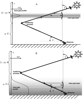
Fig. 1. Observation geometries for ground based DOAS using scat-tered sunlight: Light enters the atmosphere at a certain solar zenith angle ϑ . In the single scattering approximation light received by the observer was scattered exactly once into the telescope viewing di-rection defined by the observation elevation angle α. The observed SCD (integral along ds) is larger than the VCD (integral along dz), with AMF being the conversion factor. Panel A represents the situ-ation for a high (stratospheric) trace gas layer, panel B is represen-tative for a trace gas layer near the surface.
For a more comprehensive discussion of effects that have to be addressed when using scattered sunlight for DOAS measurements see also (Solomon, 1987b; Platt et al., 1997). 2.3 The O4spectrum
The oxygen dimer O4 is another important parameter for
MAX-DOAS. O4 is also referred to as (O2)2 to point out
that it is a collisional complex rather than a bound molecule. Absorption bands of O4occur at several wavelengths in the
UV/Vis spectral range (Perner and Platt 1980). Therefore an O4 reference spectrum (Greenblatt et al., 1990) is
of-ten included in the DOAS analysis. O4 has been used in
many cases to characterize the effects of multiple scattering in clouds and other aspects of the radiative transfer on DOAS measurements of scattered sunlight (Erle et al., 1995; Wag-ner et al., 1998; Pfeilsticker et al., 1998; WagWag-ner et al., 2002). For MAX-DOAS measurements O4can be used to determine
the importance of multiple scattering and to derive aerosol profile information (see Sect. 4, sensitivity studies, below).
3 MAX-DOAS (geometric approach)
The calculation of path average trace gas concentrations from slant column density measurements using direct sunlight or active DOAS arrangements is straightforward. In the case of the analysis and interpretation of DOAS measurements us-ing scattered sunlight, where the radiation can travel along multiple paths, it is crucial to correctly describe the radiative transfer in the atmosphere (Marquard et al., 2000). The ap-parent absorption of trace gases with distinct vertical profiles (e.g. O3, NO2, BrO) measured by a ground based
spectrome-ter depends strongly on the distribution of the paths taken by the registered photons on their way through the atmosphere. DOAS measurements using scattered sunlight yield appar-ent slant column densities (SCD) S, which are defined as the trace gas concentration integrated along the effective light path (in reality it is an average of an infinite number of dif-ferent light paths).
S = L Z
0
c(s)ds (5)
for direct light: c = S
L, c :average concentration.
Note that for a single SCD measurement the individual photons registered in the detector have travelled different paths through the atmosphere before being scattered into the DOAS telescope. Therefore Eq. (5) can only account for the most probable path defined as an average over a large number of registered photons. Since the SCD depends on the obser-vation geometry and the current meteorological conditions, it is usually converted to the vertical column density (VCD)
V, which is defined as the trace gas concentration c(z) inte-grated along the vertical path through the atmosphere:
V = ∞ Z
0
c(z)dz. (6)
The concept of air mass factors has been used for interpret-ing zenith-scattered light DOAS observations for many years (e.g. Solomon et al., 1987b; Perliski and Solomon, 1993). The air mass factor (AMF) A is defined as the ratio of SCD and VCD:
A(λ, ϑ, α, φ) = S(λ, ϑ, α, φ)
V , (7)
where ϑ denotes the solar zenith angle (SZA), α the tele-scope elevation angle and φ the relative azimuth angle, which is defined as the azimuth angle between the telescope direc-tion and the sun. Taking into account the distribudirec-tion of dif-ferent light paths leads to an improved airmass factor concept (Marquard et al., 2000).
The observation geometry and the respective angles are shown in Fig. 1. For simplicity the relative azimuth angle
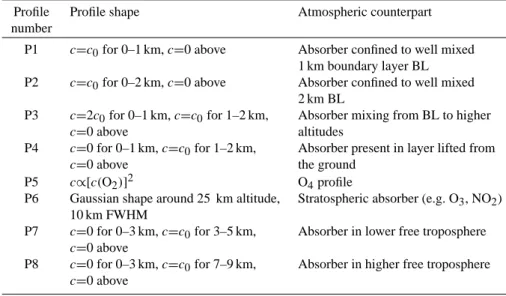
Table 2. Summary of vertical profile shapes used in this study.
Profile Profile shape Atmospheric counterpart number
P1 c=c0for 0–1 km, c=0 above Absorber confined to well mixed
1 km boundary layer BL P2 c=c0for 0–2 km, c=0 above Absorber confined to well mixed
2 km BL
P3 c=2c0for 0–1 km, c=c0for 1–2 km, Absorber mixing from BL to higher
c=0 above altitudes
P4 c=0 for 0–1 km, c=c0for 1–2 km, Absorber present in layer lifted from
c=0 above the ground
P5 c∝[c(O2)]2 O4profile
P6 Gaussian shape around 25 km altitude, Stratospheric absorber (e.g. O3, NO2) 10 km FWHM
P7 c=0 for 0–3 km, c=c0for 3–5 km, Absorber in lower free troposphere
c=0 above
P8 c=0 for 0–3 km, c=c0for 7–9 km, Absorber in higher free troposphere
c=0 above
Table 3. Summary of parameters used for the simulations in this study.
Parameter Values wavelength 352 nm
telescope elevation angle α 2◦, 5◦, 10◦, 20◦, 30◦, 40◦, 60◦, 90◦ telescope aperture angle 0.4◦
relative azimuth angle φ 90◦(2◦–180◦in Section 4.6) solar zenith angle ϑ 30◦(0◦–92◦in Section 4.7) vertical grid 100 m between 0 km and 3 km
500 m between 3 km and 5 km 1 km between 5 km and 70 km
φ is assumed to be 180◦ here. The AMF depends on the radiative transfer in the atmosphere and is therefore also in-fluenced by the profiles of several parameters including trace gas concentration, pressure, temperature, profiles of strong absorbers (e.g. ozone) and aerosols (including clouds) as well as the surface albedo.
Taking a as the fraction of the total vertical trace gas column V residing below the scattering altitude we obtain the SCD (in the single scattering approximation sketched in Fig. 1): S ≈ a · 1 sin α | {z } Alower layer (BL) +(1 − a) · 1 cos ϑ | {z } Aupper layer (strat.)
·V (a ≤1). (8)
Therefore, an absorber near the ground (e.g. in the bound-ary layer) enhances the airmass factor according to approx-imately a 1/sinα relation, expressing the strong dependence
of the AMF on the elevation angle α. In contrast, the airmass factor strongly depends on the solar zenith angle ϑ with ap-proximately a 1/cosϑ relation for an absorber in the higher atmosphere (e.g. in the stratosphere).
4 Radiative transfer calculation of MAX-DOAS air-mass factors
A set of trace gas column measurements performed at a series of different elevation angles can be used to infer the vertical trace gas profile and thus the absolute concentration of the trace gas as a function of altitude. In addition, the aerosol optical density can be quantified from the variation with the observation geometry of the SCD of species with known con-centration (such as O2and O4). An actual profile inversion
algorithm (e.g. Rodgers, 1976) was not yet implemented for MAX-DOAS at the current stage. Instead we apply the ap-proach to perform a series of simulations for a number of possible profiles and subsequently choose the “best fit” as the most likely profile. In order to characterise the role of various parameters sensitivity studies are presented here.
As mentioned above, the geometric, single scattering ap-proach using the equation A ∼1/cosϑ (for scattering below the trace gas layer), where ϑ is the solar zenith angle, or A
∼1/sinα (for scattering above the trace gas layer), where α is the telescope elevation angle, can only be regarded as an ap-proximation. In particular factors influencing the result like Mie scattering, ground albedo, or arbitrary distributions of trace gases can only be quantified by radiative transfer calcu-lations. In the following we present a study to illustrate some of the properties of the MAX-DOAS technique.
Precise air mass factors for this study were calculated us-ing the Monte Carlo radiative transfer model (RTM) “Tracy”
0 10 20 30 40 50 60 70
1E-7 1E-6 1E-5 1E-4 1E-3 0.01 0.1 1 0.00 10 20 30 40 50 60 70 80 0.2
0.4 0.6 0.8 1.0
aerosol extinction coeff. [km-1]
al tit ud e [k m ] higher stratosphere Junge layer troposphere (low load) troposphere (high load)
no rm al iz ed p ha se fu nc tio n scattering angle [°] typical continental aerosol typical marine aerosol
0 5 10 15 20 0 1 2 3 4 5 6 7 8 9 15 20 25 30 35 P1 P2 P3 P4 P5 P6 P7 P8 al tit ud e [k m ]
concentration [arbitrary units]
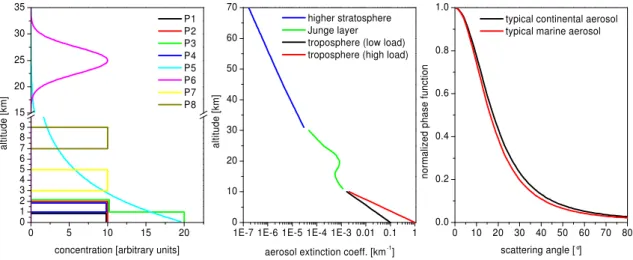
Fig. 2. Profile shapes of test profiles P1–P8 (left), aerosol profile shapes (centre) and aerosol scattering phase functions (right) used for this study (see text).
(von Friedeburg, 2003) which includes multiple Rayleigh and Mie scattering, the effect of surface albedo, refraction, and full spherical geometry. It relies on input data including pressure and temperature profiles, ground or cloud albedo, aerosol profiles and aerosol scattering phase functions as well as profiles of strong molecular absorbers like ozone. Air mass factors and other parameters like the number of scat-tering events or the altitude of the last scatscat-tering event are then calculated for various assumed profiles of the respective absorbers.
The radiative transfer may vary significantly for different angles α, ϑ or φ, therefore radiative transfer calculations were performed to quantify the influence of the above pa-rameters. In particular the behaviour of AMF’s as a function of elevation angle, solar zenith angle, solar azimuth angle, ground albedo, and aerosol load was studied for several ide-alised trace gas profiles (see Table 2 and left panel of Fig. 2). We assumed constant trace gas concentrations c in the 0– 1 km and 0–2 km layers of the atmosphere for the first four profiles (designated P1 through P4). We also investigated four further profiles for comparison, one of oxygen dimers (O4) with c∝c(O2)2(P5) and a stratospheric profile (P6,
cen-tred at 25 km with a FWHM of 10 km) as well as two free tropospheric profiles (c constant at 5±1 km and 8±1 km, re-spectively).
The dependence of the AMF for an absorber in the strato-sphere and the comparison with an absorber confined to the boundary layer has already been discussed by H¨onninger and Platt (2002) for the example of bromine oxide (BrO) in the Arctic boundary layer. The dependence on the solar azimuth angle φ was shown to be small both, for the stratospheric as well as for the boundary layer case. A significant dependence appears only for high solar zenith angles (ϑ>80◦).
The air mass factors in the sensitivity studies described below were calculated for the following set of parameters:
0 20 40 60 80 0 2 4 6 8 10 12 14 16 18 A M F elevation angle α [°] ground albedo 5% 1/sin(α) P1 P2 P3 P4 P5 P6 0 20 40 60 80 0 2 4 6 8 10 12 14 16 18 ground albedo 80% 1/sin(α) P1 P2 P3 P4 P5 P6
Fig. 3. AMF dependence on the viewing direction (elevation angle
α) for the profiles P1–P6 (see Table 2) for 5% ground albedo (left) and 80% albedo (right), respectively. Calculations were performed for a wavelength of 352 nm, 30◦Solar zenith angle, and assuming a pure Rayleigh case for the troposphere. For the stratosphere (i.e. above 10 km) the standard aerosol scenario (Fig. 2, centre panel) was assumed. The error is the intensity weighted standard deviation of the AMF averaged over the modelled photon paths. The 1/ sin(α) approximation is indicated for reference.
Wavelength λ=352 nm, Telescope elevation angles α=2◦,
5◦, 10◦, 20◦, 30◦, 40◦, 60◦, 90◦, relative azimuth φ=90◦,
ex-cept for the study of the azimuth dependence, solar zenith an-gle ϑ =30◦, except for the study of the SZA dependence. The vertical grid size h for the horizontal layers was h=100 m between 0 and 3 km, h=500 m between 3 and 5 km and
h=1 km above 5 km up to the top of the model atmosphere at 70 km. A standard atmospheric scenario (US standard at-mosphere) for temperature, pressure and ozone was used and
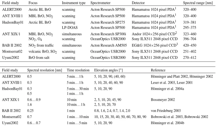
Table 4. Summary of instrumental specifications for measurements referred to in this study.
Field study Focus Instrument type Spectrometer Detector Spectral range [nm] ALERT2000 Arctic BL BrO scanning Acton Research SP500 Hamamatsu 1024 pixel PDA1 320–400
ANT XVIII/1 MBL BrO, NO2 scanning Acton Research SP500 Hamamatsu 1024 pixel PDA1 320–400
HudsonBay01 Arctic BL BrO scanning Acton Research SP275 Hamamatsu 1024 pixel PDA1 319–381 LP-DOAS Acton Research SP500 Hamamatsu 1024 pixel PDA1 295–375 ANT XIX/1 MBL BrO, NO2 simultaneous Acton Research SP300i Andor 1024×256 pixel CCD2 323–460
NO2, O4 scanning OceanOptics USB2000 Sony ILX511 2048 pixel CCD 396–704 BAB II 2002 NO2from traffic simultaneous Acton Research AM505 EG&G 1024×256 pixel CCD3 420–450
Montserrat02 volcanic BrO, SO2 scanning OceanOptics USB2000 Sony ILX511 2048 pixel CCD 251–402
Uyuni2002 BrO from salt scanning OceanOptics USB2000 Sony ILX511 2048 pixel CCD 270–412
Field study Spectral resolution [nm] Time resolution Elevation angles [◦] Reference
ALERT2000 0.5 5 min. . . 1 h 5, 10, 20, 90, (40, 60) H¨onninger and Platt 2002, H¨onninger 2002 ANT XVIII/1 0.3 5 min. . . 1 h 5, 10, 20, 40, 60, 90 Leser et al. 2003, Leser 2001
HudsonBay01 0.3 5 min. . . 30 min 5, 10, 20, 90 H¨onninger et al. 2004a 0.5 1 min. . . 1 h
ANT XIX/1 0.6. . . 0.9 10 min 2, 5, 10, 20, 45, 90 Bossmeyer 2002 1.6 10 min. . . 1 h 2, 5, 10, 20, 70
BAB II 2002 0.25 1 min 0.8, 1.6, 2.4, 0.7, 1.4, 2.0 von Friedeburg 2003
Montserrat02 0.7 1 min. . . 10 min 10, 15, 20, 30, 40, 50, 60, 70, 80, 90 Bobrowski et al. 2003, Bobrowski 2002 Uyuni2002 0.6. . . 0.7 1 min. . . 5 min 5, 10, 20, 90 H¨onninger et al. 2004b
1S59312DV420-OE31530-P-1024S
interpolated to match the vertical grid of the model. The pa-rameters used for the following simulations are summarized in Table 3.
In order to characterise the role of aerosols, the following scenarios were modelled: Above 10 km a standard aerosol load from a chemical model scenario (Hendrick, pers. comm. 2003) with εM∼10−3km−1 at 10 km was selected. Below
10 km, where the aerosol load becomes important for tropo-spheric absorbers due to its influence on the radiative trans-fer, 3 cases were chosen:
1. “Pure Rayleigh” case, no tropospheric aerosols. 2. “Low aerosol” load, with an extinction coefficient at
0 km altitude of εM=0.1 km−1, and linear interpolation
of (log εM) between the ground and the stratosphere
(see Fig. 2, centre panel).
3. “High aerosol” load with extinction coefficient at 0 km of εM=1 km−1, and linear interpolation of (log εM)
be-tween the ground and the stratosphere.
4. Two scattering phase functions were distinguished for the cases 2 and 3: (a) typical continental aerosol and (b) typical marine aerosol (see Fig. 2 right panel).
The single scattering albedo of the aerosols was set to 1 for simplicity. All model runs were performed for two ground albedo values of 5% and 80%, respectively.
4.1 The dependence of the AMF on the observation geom-etry
In order to demonstrate the sensitivity of MAX-DOAS to-wards various vertical trace gas profiles we first focus on a simple atmospheric scenario and discuss the dependence of the AMF on the viewing direction (parameterised as eleva-tion angle α) for several vertical trace gas profiles. In Fig. 3 the modelled air mass factors for the profile shapes P1–P6 are plotted as a function of the viewing direction for the pure Rayleigh case and low (left) and high (right) ground albedo. The AMF is strongly dependent on the viewing direction (elevation angle α) for the profiles, where the absorber is close to the ground. The AMF for the profiles extending to the ground (P1, P2, P3, P5) increases continuously when the elevation angle decreases. This effect can still be under-stood in the geometric approximation discussed in Sect. 3. The viewing direction determines the absorption path length, which decreases continuously for P1, P2, P3 and P5 when
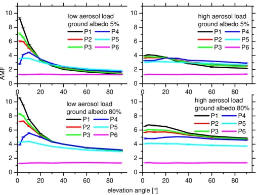
0 20 40 60 80 0 2 4 6 8
10 low aerosol load
ground albedo 5% P1 P4 P2 P5 P3 P6 A M F 0 20 40 60 80 0 2 4 6 8
10 high aerosol load
ground albedo 5% P1 P4 P2 P5 P3 P6 0 20 40 60 80 0 2 4 6 8
10 low aerosol load
ground albedo 80% P1 P4 P2 P5 P3 P6 elevation angle [°] 0 20 40 60 80 0 2 4 6 8
10 high aerosol load
ground albedo 80%
P1 P4
P2 P5
P3 P6
Fig. 4. AMF as a function of viewing direction (elevation angle α) for P1–P6 for low (left column) and high (right column) aerosol load and for 5% (top panels) and 80% (bottom panels) ground albedo, respectively. Calculations were performed for the same scenario as in Fig. 3, but for typical continental aerosol (left panels: low aerosol load, right panels: high aerosol load, see Fig. 2), differences to marine aerosol are discussed below.
P1 and less strong for the profiles extending to higher alti-tudes. The maximum AMF for the elevated layer profile P4 appears at α=5◦and AMF decreases for smaller and larger
α. Simply speaking the instrument looks “below” the layer at α<5◦. In contrast to that the AMF is almost independent of the viewing direction for the stratospheric profile P6. The characteristic altitude that determines how the AMF depends on the viewing direction is the mean last scattering altitude (LSA, see below).
4.2 Aerosol and albedo dependence
Aerosol load and scattering properties as well as the surface albedo play a significant role in the radiative transfer, espe-cially in the lower troposphere. In Fig. 4 the AMF depen-dence on the observation elevation angle is shown again for the different profile shapes (P1–P6), this time not for the pure Rayleigh troposphere, but for two different aerosol scenarios (high and low tropospheric load) as well as for high and low ground albedo. The calculations assuming low aerosol load are not different in general shape from the Rayleigh case, however the absolute values of the AMF are considerably smaller at elevation angles of 10◦and lower. In contrast, at high aerosol load the increase of the AMF at lower elevation angles becomes much weaker, and the variation of the AMF with elevation angle becomes much less pronounced.
Observer
α1
ϑ
trace gas layer Sun
α2 LSAα1
LSAα2
Fig. 5. The Last Scattering Altitude LSA: for low elevation angles, the mean free path in the viewing direction is shorter due to higher density and/or aerosol load. This can result in the slant path through absorbing layers at higher altitudes being shorter for lower elevation angles than for higher ones.
The air mass factors at low elevation angles are generally smaller for increased aerosol load compared to the Rayleigh case, while they increase at high elevation angles. However the increase of the AMF with smaller elevation angles re-mains very similar for the profiles extending to the ground (P1–P3) in the low aerosol load scenario. It can already
0 20 40 60 80 0.0 0.5 1.0 1.5 2.0 2.5 3.0 av er ag e nu m be r o f p ro ce ss es elevation angle [°] Rayleigh 80% Rayleigh 5% Albedo 80% Mie 80% Mie 5% Albedo 5%
Fig. 6. Number of Rayleigh, ground (albedo), and Mie scatter-ing events as a function of elevation angle for the typical rural low aerosol scenario and 5% (dashed lines) and 80% (drawn lines) ground albedo, respectively.
be seen in the low aerosol load scenario, that the AMF is strongly decreasing (compared to the Rayleigh case) for the profiles extending to higher levels, e.g. P4 and P5. This ap-pears to be due to the shorter mean free path of photons due to the aerosol extinction. Therefore, the absorption path in the lowest atmospheric layers is shorter in these cases and a more vertical path in the higher layers is probable as is sketched in Fig. 5. This also explains why deviations from the AMF behaviour based on simple geometric assumptions (as sketched in Fig. 1) become more and more obvious for higher aerosol loads.
This effect is even stronger for the high aerosol load sce-nario due to shorter mean free paths and correspondingly lower scattering altitudes near the ground. The maximum of the AMF curve can shift towards higher elevation angles by as much as 40◦(e.g. the lifted layer profile P4 in Fig. 4, high aerosol, 80% ground albedo case). However, shorter mean free paths also lead to a higher average number of scattering events (see Fig. 6), thus reducing the differences between the various viewing directions in a way, that differences might not be significant anymore in measurements.
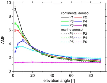
Two different aerosol phase functions, continental and maritime (see Fig. 2) were investigated, results are shown in Fig. 7. The phase function for the marine aerosol (Fig. 2) indicates slightly favoured forward scattering compared to the continental case. However, no significant differences be-tween the two aerosol types can be seen here, since the phase functions are quite similar.
The effect of higher albedo generally enhances the AMF for the profiles extending to the ground (P1–P3), because longer absorption paths in the lowest layers are favoured by scattering at the ground. Since the effect of the higher albedo increases all AMF’s by almost the same amount, it has no
0 20 40 60 80 0 2 4 6 8 10 A M F elevation angle [°] continental aerosol P1 P2 P3 P4 P5 P6 marine aerosol P1 P2 P3 P4 P5 P6
Fig. 7. Effect of different aerosol types on the AMF, drawn lines in-dicate continental background aerosol (same as “low aerosol load” in Fig. 4). Only small differences result from different scattering phase functions.
significant effect on the elevation angle dependencies, and rather constitutes an offset.
As mentioned above, another parameter that determines the sensitivity of MAX-DOAS towards absorbers with dif-ferent profile shapes is the number of scattering events that photons undergo on average prior to being detected by the MAX-DOAS instrument. Figure 6 shows the contribution of the different scattering processes as a function of elevation angle for the typical low aerosol scenario for both low (5%) and high (80%) ground albedo.
It can clearly be seen that a higher ground albedo strongly increases the overall number of scattering events compared to the low albedo case. The probability of Mie and ground scat-tering processes increases, especially for the low elevation angles. Since both scattering processes take place largely at or close to the ground, this finding is not surprising. How-ever, the specific behaviour and the influence on the respec-tive air mass factors can only be modelled properly using an RTM. The albedo increase from 5% to 80% has also a signifi-cant effect on the number of Rayleigh scattering events, since more light reaching the ground is reflected and can undergo more scattering processes.
4.3 The Last Scattering Altitude (LSA)
A key parameter that governs the sensitivity of MAX-DOAS measurements towards different vertical profiles of absorbers is the altitude of the last scattering event (last scattering alti-tude, LSA, see also Fig. 5) before the photon finally reaches the MAX-DOAS instrument. The LSA dependence on the viewing direction is shown in Fig. 8. As expected, the LSA becomes smaller for the lower elevation angles. This can lead to the observed behaviour of the AMF with a maximum
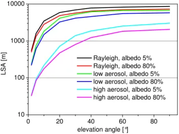
0 20 40 60 80 10 100 1000 10000 LS A [m ] elevation angle [°] Rayleigh, albedo 5% Rayleigh, albedo 80% low aerosol, albedo 5% low aerosol, albedo 80% high aerosol, albedo 5% high aerosol, albedo 80%
Fig. 8. Last scattering altitude (LSA) for pure Rayleigh, low and high aerosol load scenarios (see Fig. 4) and both, 5% and 80% albedo. The LSA is generally below 1km for the lowest elevation angle and above 1km for the highest elevation angles, especially for zenith viewing direction.
between 10◦and 20◦, and smaller AMF for the very low el-evation angles (e.g. for P3). The LSA effectively determines the length of the last section of the path taken by the pho-tons through the lowest atmospheric layer at the observation elevation angle α.
This analysis explains the following effects:
– For profiles extending to the ground and with vertical
extensions comparable to the LSA, such as P1–P3, the AMF is generally smaller than estimated from the geo-metrical (1/sinα)-approximation.
– For profiles elevated from the ground and/or with a
sig-nificant fraction of the profile above the respective LSA, such as P4 or P5, the AMF has a maximum at an eleva-tion angle, where the mean free path still allows tran-secting the absorbing layer on a long slant path. AMF’s decrease again for the very small elevation angles due to light paths being shorter in the layers with high absorber concentrations.
– For stratospheric profiles, such as P6, the last
scat-tering processes near the ground cannot influence the AMF since the absorber is only present at high alti-tudes. Therefore, the AMF for stratospheric absorbers is largely independent of the viewing direction. 4.4 “Box” air mass factors
Box AMF’s are a measure of the light path enhancement compared to a vertical path in a given height interval. In
0 2 4 6 8 10 12 14 16 18 20 22 24 26 28 30 0 5 10 15 20 25 B ox A M F elevation angle [°] 0-100 m 100-200 m 200-300 m 300-400 m 400-500 m 500-600 m 600-700 m 700-800 m 800-900 m 900-1000 m 1000-1100 m 1100-1200 m 1200-1300 m 1300-1400 m 1400-1500 m 1500-1600 m 1600-1700 m 1700-1800 m 1800-1900 m 1900-2000 m
Fig. 9. Box AMF for the model layers below 2 km altitude. The sensitivity towards the lowest layers changes strongly for elevation angles below 10◦, for elevation angles smaller than 5◦the sensitiv-ity already decreases for layers above 400 m altitude.
the case of weak absorption and a horizontally homogeneous atmosphere the Box AMF can be expressed as:
ABox= R Box ds R Box dz, (9)
with the actual light path s and the vertical path z.
Box Air Mass Factors modelled for different viewing di-rections (elevation angles) therefore serve as a measure of the sensitivity of a particular viewing direction towards an absorber being present in a specific vertical “box” (or layer). Therefore, Box AMF’s provide a criterion for determining the sensitivity of MAX-DOAS for different shapes of verti-cal profiles.
Figure 9 shows modelled Box AMF’s for assumed trace gas layers of 100 m thickness located below 2 km altitude. Variations of the Box AMF’s are clearly strongest towards the surface for the very low elevation angles. Consequently MAX-DOAS should be very sensitive to different profile shapes in this altitude range. The general trend for eleva-tion angles smaller than 5◦of increasing Box AMF with de-creasing α is only observed for layers below 400 m altitude. Above this altitude, the trend reverses and Box AMF’s de-crease.
This confirms that a good knowledge of the aerosol load of the probed airmass is important in order to choose the cor-rect AMF and thus to derive quantitative trace gas vertical columns V . In fact, some information about the vertical trace gas distribution can be gained from an analysis of the vari-ation of the observed slant column with the elevvari-ation angle, as explained above; the vertical thickness D of a trace gas layer can be derived. This information can be used to infer the average trace gas concentration in the layer.
Determine Slant Column Densities at Several Elevation Angles
Determine Aerosol Load from O4
Calculate Appropriate Airmass Factors
Determine „Best Fit“ Vertical Trace Gas Profile
Fig. 10. Diagram of a MAX-DOAS evaluation procedure including the determination of the aerosol load from O4observations.
4.5 O4profile and measurements as good indicator for the
aerosol load
The observation of the slant columns of oxygen dimers (and other species with known atmospheric distribution, e.g. O2)
offers in principle an excellent opportunity to determine the aerosol load of the atmosphere. The atmospheric O4
con-centration profile is well known; it is essentially given by
cO4(z)∝c
2
air(z)with a known dependency of the air density
cair on temperature and barometric pressure. The measured
set of O4slant column densities (for a series of elevation
an-gles e.g. from 2◦to 90◦) can then be compared to a series of calculated O4SCD’s (for the temperature and pressure
pro-file as recorded during the measurement), where the aerosol load should be varied until best agreement is reached. As outlined in Fig. 10 this aerosol load can then be used to cal-culate a further series of “Box” AMF’s which, together with the slant column densities of the trace gases under investiga-tion, can be used as input for a linear equation system. Alter-natively, the AMF for several test profiles can be calculated and the “best fit” vertical trace gas profile (of e.g. the type P1...P4) can be chosen.
4.6 Azimuth dependence of the AMF
In the case of horizontally inhomogeneous trace gas distri-butions the observation azimuth angle is clearly of impor-tance and has to be determined in each individual case. For horizontally homogeneous distributions a dependence of the air mass factors on the relative azimuth angle between the sun and the viewing direction can arise from the shape of scattering phase functions for the respective scattering pro-cesses. Therefore, light paths taken by photons at different relative azimuth angles may be different resulting in differ-ent elevation angle dependence of the AMF and possible results on MAX-DOAS measurements. This effect is ex-pected to be higher for large SZA since only then can one expect significant influence on the radiative transfer at low altitudes which is most important for MAX-DOAS measure-ments (H¨onninger and Platt, 2002).
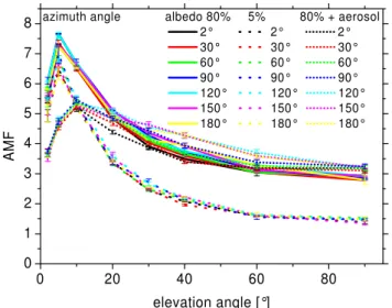
0 20 40 60 80 0 1 2 3 4 5 6 7 8 A M F elevation angle [°]
azimuth angle albedo 80% 5% 80% + aerosol 2° 2° 2° 30° 30° 30° 60° 60° 60° 90° 90° 90° 120° 120° 120° 150° 150° 150° 180° 180° 180°
Fig. 11. Azimuth-dependence of the AMF for 30◦SZA and profile P4 (trace gas layer at 1–2 km altitude). For relative azimuth an-gles between 2◦(looking almost towards the sun) and 180◦ (look-ing away from the sun) only a small effect increas(look-ing with ground albedo and aerosol load can be seen. Calculations were performed for a ground albedo of 80% and 5% (cf. Fig. 3) in the Rayleigh case (in the troposphere) and for 80% ground albedo in the low aerosol case (cf. Fig. 4).
Figure 11 shows the small effect of the relative azimuth an-gle for a SZA of 30◦and the profile P4. No significant influ-ence on the general elevation angle dependinflu-ence of the AMF is seen. However, the small azimuth dependence is found to increase with ground albedo and tropospheric aerosol load. 4.7 SZA dependence of the AMF
The solar zenith angle (SZA) is the most important parame-ter when characparame-terizing air mass factors for stratospheric ab-sorbers. In Fig. 12 the strong dependence of the AMF on the SZA can be seen for the stratospheric profile P6, whereas the viewing direction only plays an insignificant role. In contrast to that for the tropospheric profiles (e.g. P2 and the O4profile
P5) the SZA dependence of the AMF is minor and only sig-nificant at large SZA. Here, the viewing direction (elevation angle) is the parameter that governs the AMF as discussed above.
The SZA dependence of the AMF for the different profiles can be best understood from the altitudes of the first and last scattering event (FSA, LSA, respectively). These parame-ters can serve as a proxy for the general pattern of the light path taken by the registered photons. Figure 13 shows both first and last scattering altitude as a function of SZA. While the FSA strongly increases towards high SZA, the LSA is largely independent of SZA. As long as the FSA is below or still within an absorber profile (which is the case for the O4
profile P5 up to a higher SZA than is the case for P2), the first light path segment (above FSA) increases strongly with
0 20 40 60 80 0 5 10 15 20 25 0 20 40 60 80 0 20 40 60 80 0 5 10 15 20 25 A M F P6 2° 5° 10° 20° 30° 40° 60° 90° SZA [°] P2 P5
Fig. 12. Solar Zenith angle (SZA) – dependence of the AMF for the typical stratospheric profile P6 and the boundary layer profile P2 as well as the O4profile P5 for comparison. The expected strong dependence is observed for the stratospheric absorber, with no significant
dependence on the viewing direction. In contrast to that for the tropospheric profiles P2 and P5 significant differences for the various viewing directions can be seen, whereas the SZA dependence is significant only at higher SZA (i.e. >70◦).
0 10 20 30 40 50 60 70 80 90 0.0 0.2 0.4 0.6 0.8 10 20 30 40 al tit ud e [k m ] SZA [°] FSA LSA
Fig. 13. First and last scattering altitude for the 2◦elevation angle. The FSA strongly depends on the SZA, whereas the LSA is largely independent of the SZA. Note the axis break at 1km altitude and the expanded y-scale below.
SZA (approximately according to 1/cos(SZA)). As soon as the FSA is above the absorber, the first slant path segment does not increase the AMF and therefore the AMF depen-dence on the SZA disappears.
4.8 Profiles of free tropospheric absorbers
As discussed above, ground-based MAX-DOAS can clearly distinguish between stratospheric profiles (e.g. P6) and vari-ous tropospheric profiles (P1–P5). However, the limitation of
0 20 40 60 80 0 1 2 3 4 5 6 0 20 40 60 80 2° 30° 5° 40° 10° 60° 20° 90° A M F SZA [°] P7 2° 30° 5° 40° 10° 60° 20° 90° P8
Fig. 14. AMF as a function of SZA for the “free tropospheric pro-files” P7 and P8 with the elevation angle as parameter (shown in dif-ferent colors). The SZA dependence is smaller than for the strato-spheric profile P6, but much stronger than for the lower tropostrato-spheric profiles P1–P5.
the sensitivity towards profiles at higher altitudes remains to be investigated. Figure 14 shows the SZA dependence of the AMF for two layers with constant trace gas concentration in the free troposphere (P7 and P8, see Table 2 for definition).
The SZA dependence of the profiles P7 and P8 is not as strong as for the stratospheric profile P6, but clearly more visible than for the boundary layer profiles or the O4profile
P1–P5. On the other hand, the differences between the var-ious elevation angles (shown as different colours in Fig. 14) are much smaller than for the lower tropospheric profiles.
Miniature
Spectrometer
(Peltier-cooled) Entrance opticsInsulation
To PC 20 cm M ec ha ni ca l po in tin g de vi ce (c om pu te r c on tr ol le d)Fig. 15. Outline of the Mini-MAX-DOAS instrument. A minia-ture spectrometer is cooled and temperaminia-ture stabilized by a 2 stage Peltier cooler. The built-in entrance optics (telescope) provide a narrow field of view (<0.5◦). The unit can be pointed in various directions by computer control.
Differences for various elevation angles are still significant in MAX-DOAS measurements for a free tropospheric profile like P7, however, for profile P8 the small differences between the viewing directions are even more difficult to measure and to distinguish from measurement errors, modelling noise and from the variability of the trace gas concentration.
5 Practical realization of MAX-DOAS systems
As described above MAX-DOAS systems have been em-ployed for the measurement of atmospheric trace gases by several authors (see Table 1). A number of technical re-quirements have to be fulfilled by MAX-DOAS instruments. Besides sufficient spectral resolution (around 0.5 nm in the near UV) in particular a sufficiently small field of view of the telescope (typically <1◦) is required, and of course the instrument must allow measurements in different viewing di-rections. A number of technical approaches have been devel-oped to meet these requirements:
1. Sequential observation at different elevation angles. This approach has the advantage of a relatively sim-ple set-up requiring only one spectrometer and some mechanism for pointing the telescope (or the en-tire spectrometer-telescope assembly) in the desired directions. It was therefore used in several stud-ies (H¨onninger and Platt, 2002; Leser et al., 2003; Bobrowski et al., 2003; H¨onninger et al., 2004a; H¨onninger et al., 2004b). Disadvantages are that the measurements are not simultaneous, typically a complete cycle encompassing several (usually 4 to
10) observation directions may take 5 to 30 min (e.g. H¨onninger and Platt, 2002). It certainly depends on the respective aim of a field study whether this represents a significant drawback. For example, at high latitudes simultaneity may often not be an issue because the SZA changes only slowly there. In contrast to that the effect of changing SZA and thus the observed stratospheric trace gas column densities is much more pronounced at mid- and low latitudes. However, since the change in SZA can be well described by a simple polynomial fit to the measured time series for each elevation angle, its effect can be removed by interpolating all time se-ries on a common grid prior to further analysis (Leser et al., 2003). On the other hand interpolation can be diffi-cult during periods of rapidly varying radiative transport conditions in the atmosphere, for example varying cloud cover, aerosol load, during sunrise/sunset or on a mov-ing (e.g. airborne) platform. In the latter cases and when high time resolution is required simultaneous observa-tion should be preferred (see below). A scanning instru-ment also contains mechanically moving parts, which may be a disadvantage in long term operation at remote sites. Very robust, lightweight and small-sized Mini-MAX-DOAS instruments have recently been applied for automated operation at remote sites (Galle et al., 2003; Bobrowski et al., 2003; H¨onninger et al., 2004b) (see Fig. 15).
2. Simultaneous observation at different elevation angles allows truly simultaneous determination of SCD’s at the different elevation angles and thus avoids the problems of set-up 1. Disadvantages here are the larger instru-mental requirement, since a spectrometer and a tele-scope for each of the observation directions is needed. However, recent development of very compact, low cost spectrometer/detector combinations (e.g. Galle et al., 2003; Bobrowski et al., 2003; H¨onninger et al. 2004b see Fig. 15) can be of help here. Simultaneous measure-ments can be realised by installing a set of instrumeasure-ments observing multiple elevation angles from the same lo-cation. In case of non-homogeneous trace gas distribu-tions this approach is superior to the scanning method, since additionally scanning the azimuth angle further decreases the time resolution. Alternatively some sim-plification may come from using spectrometers with two dimensional detectors, (see Fig. 16 and description below) (Heismann, 1996; Wagner et al., 2002; L¨owe et al., 2002; Bossmeyer, 2002; Oetjen, 2002; von Friede-burg, 2003; Heckel, 2003).
A severe problem arises, however, if the different in-struments are to be ratioed against each other in order to eliminate the solar Fraunhofer structure (see Sect. 2). This proves extremely difficult if different instruments with – in practice – different instrument functions are involved (e.g. Bossmeyer, 2002; von Friedeburg, 2003).
Entrance slit
CCD detector at the focal plane of the
spectrograph
λ (x) y
End of the fibre bundle
Fig. 16. Two dimensional spectrometer: Orientation of the spec-tra of the measured light from different viewing angles on the CCD array. The dispersion direction is labeled “x”, thus for each fibre ending at the entrance slit a complete and separate spectrum is gen-erated on the CCD.
Although this can in principle be overcome by “cross convolution” (i.e. convolving each measured spectrum with the instrumental line shape of the respective spec-trum it is to be compared with), or by generating dif-ference spectra from FRS, none of these approaches has yet provided the same sensitivity as can be reached with a scanning instrument. Any convolution of measured atmospheric spectra with an instrument function of typ-ically 5–10 detector pixels FWHM reduces the spectral resolution and essentially “smoothes” intensity varia-tions (e.g. spectral features, photon shot noise, detec-tor pixel-to-pixel variability and electronic noise) that are below the spectral resolution (FWHM) of the in-strument. This can result in spectral artefacts due to smoothing of noise and thus can affect the quality of the DOAS fit (e.g. Bossmeyer, 2002). While detector pixel-to-pixel variability can largely be removed by cor-recting with a “white light” spectrum (e.g. from an in-candescent lamp), taking these additional spectra regu-larly comes at the cost of measurement time, additional power requirements and experimental effort. It appears that, given present instrumentation, the highest sensitiv-ity is reached with sequential observation.
3. A solution lies in the combination of techniques 1) and 2), i.e. the use of multiple spectrometers (one per obser-vation direction) and moving telescopes (or spectrome-ter telescope assemblies). While this approach appears to combine the disadvantages of the two above set-ups it also combines their advantages: If each individual in-strument sequentially observes at all elevation angles and the observations are phased in such a way that at any given time one instrument observes each observa-tion direcobserva-tion, then indeed not only will simultaneous observation be achieved at each angle, but also each instrument regularly sees the zenith to record a
Fraun-0.0 0.5 1.0 1.5 2.0 2.5 0.0 0.1 0.2 0.3 0.4 0.5 0.0 0.5 1.0 1.5 2.0 2.5 2 5 10 20 90 α-1 [deg-1] elevation angle α [°] ∆ S C D B rO [1 0 14 cm -2 ] measured modelled P1 (0-1km) P2 (0-2km) P3 (0-1km+1-2km) P4 (1-2km) P5 (O4) P6 (strat.)
Fig. 17. Comparison of 1SCD’s measured on 4 May 2000 (15:15 UT–15:40 UT) during the Alert2000 field experiment by H¨onninger and Platt (2000) with calculated 1SCD’s for assumed profile shapes P1–P6 as a function of the elevation angle α. For bet-ter illustration the x-axis was chosen linear in α−1. 4 May 2000 at Alert was characterized by a relatively constant BrO column (BL-VCDBrO=2×10¹³molec/cm2). Only P1 is compatible with the measured values.
hofer spectrum for reference. Instruments based on this approach are presently used on cruises of the German research vessel Polarstern (see Leser et al., 2003; Boss-meyer, 2002).
5.1 Spectrometer with two dimensional detector for simul-taneous MAX-DOAS observation
In the simultaneous MAX-DOAS version light from several telescopes collecting scattered sunlight at the desired eleva-tion angles is transmitted to the entrance slit of the spec-trometer by quartz fibres (see Fig. 16). In order to sepa-rate the spectra of the light observed at the different viewing angles two-dimensional CCD arrays are needed as detectors (Heismann, 1996). The light is dispersed in λ (x)-direction (Fig. 16) and the different spectra for the light from differ-ent fibres are separated in y-direction (with each spectrum covering several rows of the CCD array). Thus it is possi-ble to measure the different spectra simultaneously. Unfor-tunately the instrumental transmission function for the indi-vidual viewing directions may not be sufficiently similar to allow ratioing to the zenith, thus two dimensional spectrom-eters are best combined with technique 3 (see above).
21 Apr 24 Apr 28 Apr 2 May 5 May -2 0 2 4 6 0 2 4 6 8 10 0 1 2 3 4 -10 1 2 3 4 5 elevation angles 5°10°20°40°60°90° O4 [a .u .] Date 2000 [UT] B rO [1 0 14 cm -2 ] N O2 [1 0 16 cm -2 ] O3 [1 0 19 cm -2 ]
Fig. 18. MAX-DOAS time series of DSCD’s of O3, NO2, O4and BrO at Alert during spring of 2000. Error bars (2σ ) are shown in light
grey. The O3and NO2columns show no variation for the different elevation angles indicating that the bulk of these species is located in
the stratosphere. In contrast to that the O4data vary strongly with elevation angle. Enhanced O4levels around 27/28 April at high elevation angles indicate periods of snowdrift. Following 27 April the BrO columns show strong differences for different elevation angles due to BrO presence in the boundary layer. Effects of snowdrift on 27/28 April can be seen like for O4.
6 MAX-DOAS observations
6.1 Comparison of measured and modelled SCD’s As discussed above, RTM calculations yield airmass fac-tors for a priori trace gas profiles with the elevation angle as important parameter. This permits the derivation of ver-tical profile information from actual MAX-DOAS measure-ments. DSCD’s, which result from the MAX-DOAS anal-ysis for different elevation angles, are usually differential SCD’s with respect to a Fraunhofer reference spectrum taken at the zenith viewing direction. In order to eliminate pos-sible bias 1SCD’s are either directly derived by choosing a spectrum taken simultaneously or within short time as Fraun-hofer reference for the DOAS analysis. This procedure yields
1SCD’s, which can also be calculated from DSCD’s (when only a single FRS was taken for the entire DOAS analysis) as shown in Sect. 2 above.
Here α=90◦was assumed for recording the FRS, however, in special cases a different viewing direction could be chosen for the FRS.
Figure 17 shows an example for measurements taken dur-ing the Polar Sunrise Experiment Alert 2000 by H¨onndur-inger and Platt (2002). Measured data points (1SCD’s) are plot-ted as a function of the elevation angle. Additionally the model predicted 1SCD’s calculated from the boundary layer column BL-VCD=2×1013cm−2 and the differential AMF
1AMF(α)=A (α)−A (α=90◦) are shown for the model lay-ers P1-P6. The measured values agree well with the model results for P1, representing a constant trace gas profile over the lowest 1 km of the atmosphere. The other profiles are not compatible with the measured data in this case. It can also be seen that the most significant differences between the modelled 1SCD’s for the various profiles appear at the low elevation angles. For deriving vertical profile information us-ing MAX-DOAS, measurements at low elevation angles are therefore crucial.
First MAX-DOAS observations of BrO in the Arctic boundary layer (Alert, 82.5◦N) during spring of 2000 were already reported by H¨onninger and Platt (2002). Here we show a more comprehensive data set including stratospheric absorbers and O4. Figure 18 shows the MAX-DOAS
re-sults (time series of 3 weeks), where the change in solar zenith angle is very small compared to mid-latitudes (di-urnal 1SZA=15◦). O
3 and NO2 show the typical pattern
of stratospheric absorbers, which only depend on the SZA. Changes in tropospheric O3are masked by the large
strato-spheric O3column. The vertical ozone column changes only
by about 1% in the high Arctic during polar sunrise, where the whole boundary layer ozone column is destroyed during frequent episodes of boundary layer ozone depletion. With the AMF for the stratospheric ozone column in the range of 5 at SZA=80◦, even the high sensitivity of MAX-DOAS at the surface is not sufficient to measure this effect of typically
08:00 12:00 16:00 0 5 10 O 4 O D @ 3 80 .2 n m [x 10 -3 ] October 1, 2000 08:00 12:00 16:00 October 9, 2000 elevation angleα 90° 60° 40° 20° 10° 5°
Fig. 19. O4absorption at different elevation angles in mid-latitudes. Clearly visible is the pattern of increasing O4absorption with decreasing elevation angle. The regular pattern shown for a cloud-free day on the right is disturbed only for the lowest elevation angles on a cloudy day (left). The Multi Axis effect is much stronger than the overlaid U-shape pattern which is due to the change in SZA (Leser, 2001; Leser et al., 2003).
08:00
12:00
16:00
0
5
10
15
October 1, 2000
N
O
2D
S
C
D
[x
10
16cm
-2]
08:00 12:00 16:00
elevation angleα 90° 60° 40° 20° 10° 5°October 12, 2000
Fig. 20. Shown are two examples of NO2DSCD’s, one for a case with pollution observed in the lower troposphere (left panel, North Sea,
1 October 2000), the right panel shows stratospheric background NO2only with no significant differences between the individual elevation angles (Leser, 2001; Leser et al., 2003).
2–3%. In the NO2time series several pollution events (21,
22, 26 April, 7 May) can be identified as low elevation angle data points deviating from the general pattern which tracks the SZA change. These episodes are always correlated to exhaust plumes being blown into the MAX-DOAS viewing direction which originated either from a nearby generator or from the Alert base at several kilometres distance. On 27 April 2000 BrO 1SCD’s rise from background levels of
<1013molec/cm2up to 1015molec/cm2and simultaneously large differences can be seen between the used MAX-DOAS elevation angles. H¨onninger and Platt (2002) inferred a BrO layer of roughly 1 km thickness at the surface from the MAX-DOAS results at 4 different elevation angles using only single scattering RTM calculations. Episodes of drifting snow (e.g. on 27/28 April) can also be modelled with the new RTM by von Friedeburg (2003). Also a more comprehensive
investi-gation of the evolvement of the BrO layer over time is pos-sible (von Friedeburg, 2003). O4 shows very little diurnal
variation but the typical change in absorption with changing elevation angle for a lower tropospheric absorber. Effects of multiple scattering can be seen for the drifting snow period between 26 and 29 April (H¨onninger, 2002). The measured column densities are elevated for all viewing directions as a result of enhanced light path lengths in the lowest atmo-spheric layer. Additional information on the aerosol profile can be derived by applying the approach mentioned above (see Sect. 4, sensitivity studies O4).
Another example illustrating the effects of clouds on the radiative transfer and the detection by MAX-DOAS is shown in Fig. 19 for measurements at mid-latitudes. Ship borne MAX-DOAS measurements of BrO, NO2 and O4 were
16 18 20 22 00 0 5 10 15 20 B rO ∆ S C D [1 0 14 cm -2 ]
MAX-DOAS elevation angle 5° 10°
20°
Time (UTC) on April 27, 2001
M A X -D O A S B rO [p pt * ] (5 ° on ly ) 0 5 10 15 20 16 18 20 22 00 0 5 10 15 20 Active DOAS LP -D O A S B rO [p pt ] 0 1 2 3 4 5
Fig. 21. Comparison of active long path DOAS and passive MAX-DOAS BrO measurements at the Hudson Bay for 27 April 2001. From the elevation angle dependence of the 1SCD’s a ∼1 km BrO layer at the surface can be concluded for e.g. 16:00 h. Using this layer thickness the 5◦BrO 1SCD’s were converted to mixing ratios for better comparison with the long path DOAS data (H¨onninger et al., 2003a).
FS Polarstern from Bremerhaven, Germany to Cape Town, South Africa (Leser, 2001; Leser et al., 2003). A major dif-ference in comparison with the above example at high lati-tudes is the range of the solar zenith angle over the course of the day. In Fig. 19 the strong influence of the change in SZA on the MAX-DOAS measurements can be seen as U-shaped diurnal pattern. Leser et al. (2003) presented a method to account for the change in SZA during sequential MAX-DOAS measurements by fitting a polynomial function to the diurnal DSCD pattern and calculating 1SCD’s using interpolated values for SCDFRS. This method was applied
successfully for measurements at mid-latitudes by Leser et al. (2003). On the partly cloudy day shown in Fig. 19 (left) enhanced DSCD’s due to light path enhancement in clouds are seen for the lowest elevation angles (5◦, 10◦and 20◦).
Another application of ground-based MAX-DOAS is the study of tropospheric pollutants like NO2and SO2. During
the ship borne MAX-DOAS measurements by (Leser, 2001; Leser et al., 2003) it was also possible to study pollution episodes. Figure 20 demonstrates the sensitivity of MAX-DOAS to NO2in the boundary layer in the North Sea. During
enhanced NO2levels in the boundary layer the typical
pat-tern of strongly increasing DSCD with decreasing elevation angle is found on 1 October 2000 (Fig. 20, left panel) when the ship cruised in the North Sea. On 12 October 2000 a typ-ical U-shaped diurnal pattern of DSCD’s with no significant differences between the measurements at various elevation angles shown in Fig. 20 (right panel) represents stratospheric background NO2and an unpolluted troposphere.
7 Comparison of passive MAX-DOAS with active long path-DOAS
During a field campaign at the south-east shore of the Hud-son Bay, Canada, simultaneous measurements of BrO using an active Long path-DOAS system (e.g. Platt 1994) and a passive MAX-DOAS instrument were performed. The active long path DOAS yielded average BrO concentrations over a 7.6 km light path at ∼30 m altitude above the sea ice surface. The passive MAX-DOAS was also set-up on a hill ∼30 m above the sea ice. It used elevation angles of 5◦, 10◦, 20◦ and 90◦above the horizon and the viewing azimuth was true north, less than 10◦relative to the long path DOAS light path, so the same airmass was sampled in both cases (H¨onninger et al., 2004a).
An example of the intercomparison results is shown in Fig. 21. From noon to sunset the BrO as measured by the long path DOAS system showed high BrO values of 18 ppt BrO at noon decreasing to <5 ppt in the evening. The MAX-DOAS BrO 1SCD’s are shown in the lower part of Fig. 21 for the elevation angles of 5◦, 10◦and 20◦. Around 16:00 h
the elevation angle dependence compares best with a ∼1 km BrO layer at the surface. Therefore, the 5◦ 1SCD’s were converted to mixing ratios using this assumption. Indeed, the absolute values of the MAX-DOAS mixing ratios (black data points and line in Fig. 21, bottom panel) match the Long path-DOAS data (top panel of Fig. 21) very well. Small differences can be explained by variability of the boundary layer thickness. It can also be seen that the time resolution